Abstract
Crowd logistics is a recent trend that proposes the participation of ordinary people in the distribution process of products and goods. This idea is becoming increasingly important to both delivery and retail companies, because it allows them to reduce their delivery costs and, hence, to increase the sustainability of the company. One way to obtain these reductions is to hire external drivers who use their own vehicles to make deliveries to destinations which are close to their daily trips from work to home, for instance. This situation is modelled as the Vehicle Routing Problem with Occasional Drivers (VRPOD), which seeks to minimize the total cost incurred to perform the deliveries using vehicles belonging to the company and occasionally hiring regular citizens to make just one delivery. However, the integration of this features into the distribution system of a company requires a fast and efficient algorithm. In this paper, we propose three different implementations based on the Iterated Local Search algorithm that are able to outperform the state-of-art of this problem with regard to the quality performance. Besides, our proposal is a light-weight algorithm which can produce results in small computation times, allowing its integration into corporate information systems.
1. Introduction
Nowadays, many people use e-commerce to buy and sell all kind of goods, products and services. The 24/7 availability of the websites, the wide array of products and services, the easy reachability to get any of them in any place, the easy way of comparing prices and the possibility of gather opinions from other customers are some of the advantages that support the use of the e-commerce. These reasons, together with the lack of time of most citizens, make e-commerce continue to grow, which leads to an increase on the delivery services, especially in the last-mile operations [1].
Both delivery companies and retailers which also distribute their products strive to minimize the total cost and the delivery time to be more efficient [2]. However, the increase of delivery operations impacts on the sustainability of a company, either by enlarging the routes or by performing door-to-door distributions, which could require increasing the number of vehicles attending customers [3]. In an early stage of the last-mile development, [4] held that the cost related to the last-mile operation may range between 13 and 75% of the total distribution cost. Therefore, the optimization of this step of the supply chain led to an important reduction on the distribution costs for many delivery companies that focused on solving the last-mile problem to reduce costs. Since then, many delivery companies have focused on reducing this cost, but it is important to emphasize that this range may vary significantly depending on the specific problem under consideration.
Recently, a new trend called crowd logistics is gaining relevance [5,6,7]. The idea behind this concept is to favor the participation of ordinary citizens in the distribution of goods. The authors of [6] distinguish between four types of crowd logistics: crowd storage, crowd local delivery, crowd freight shipping and crowd freight forwarding. We will only focus on one of them: the crowd local delivery or crowdshipping, as called by other authors [8]. In particular, the key concept of crowdshipping here is to either deliver orders through other customers, or hire regular people close to the delivery route to occasionally perform a delivery on behalf of a logistics operator. The implementation of this idea may contribute to the sustainability of a company because it will reduce the logistics network [6] and, eventually, reduce the urban traffic levels [9] as well as the logistics costs [10]. In addition, this can be an opportunity to obtain extra incomes for the occasional couriers at the cost of slightly modifying their daily route from work to home or vice versa [6]. Note that crowshipping can be seen as an example of sustainable transportation apart from other typical examples such as walking, cycling, carpooling, car sharing, or green vehicles [11].
The concept of crowd logistics is mainly related to the vehicle routing problem (VRP). The VRP aims to find the best routes to satisfy the demand of a set of customers, given a fleet of vehicles [12,13]. Therefore, since crowd logistics involves the last-mile operations, it can be tackled from the VRP point of view.
In this paper we propose a light-weight and efficient algorithm to optimize the last-mile logistics including the concept of crowdshipping. As it is well-known, the last-mile delivery problem consists on the transportation of the goods from the warehouse, called depot in this work, and the final destination, usually the customer’s home or business. Last-mile problems are considered very important regarding sustainability since they involve the less efficient phase of the logistic process [14]. Furthermore, in this work, we consider those deliveries to be performed by ordinary citizens, the occasional drivers, as part of a crowdshipping strategy, in addition to the own staff of the delivery company. Previous works like [15] describe the impact on sustainability of this kind of distribution models.
Given the small computation time and low complexity of our algorithm, it can be included in a corporate information system with the objective of optimizing a set of delivery orders taking into account both delivery routes and occasional couriers. Hence, a company will be able to reduce its costs and increase its sustainability levels by hiring occasional couriers, since the proposed algorithm is able to optimize the last mile routes taking into account the collaboration of occasional drivers.
In order to assess our proposal, we have studied the Vehicle Routing Problem with Occasional Drivers (VRPOD). VRPOD is able to model last-mile situations appearing in delivery companies that allow crowdshipping in addition to their own staff. The VRPOD assumes that the company has a fleet of vehicles handled by regular drivers who make deliveries limited by the capacity of the vehicles. Furthermore, the company is able to hire a number of occasional drivers to make a single delivery using their own vehicles. The objective of the VRPOD is to minimize the total cost, calculated as the sum of the costs incurred by the regular drivers performing traditional routes, beginning and ending at the depot, plus the cost of paying the occasional drivers, since they provide their service in exchange of remuneration. To the best of our knowledge, this problem was firstly defined by [16], who studied the potential benefits of including occasional drivers to make deliveries as a way of crowdshipping. The authors considered two compensation schemes to pay fixed fees to every occasional driver.
Since then, new variants of the VRPOD have been analyzed. In the work proposed in [17], the authors considered that occasional drivers appear dynamically and they assume that stochastic information is known about this behaviour. Furthermore, occasional drivers could serve one or more of the customers. The authors propose a stochastic mixed-integer programming formulation to solve the problem. They study the effects of uncertainty to design the routes when the occasional drivers can appear later in the day. A similar work by [18] includes two aspects: the possibility for occasional drivers to make multiple deliveries and the time windows for the customers and so the occasional drivers. The authors study the advantages of employing two different alternatives: occasional drivers that are allowed to perform multiple deliveries and occasional drivers that can split the deliveries. Their proposal is proven using two different mathematical models. Later on, a variant of the VRPOD in which occasional drivers may accept or reject the assigned delivery with a certain probability was presented in [19]. The authors solve the problem with a bi-level methodology in which they start by including all the deliveries in regular routes without the use of occasional drivers, and then include deliveries to occasional drivers taking into account their acceptance probabilities modelled using a uniform distribution.
There exist other problems related to the VRPOD although they present some differences since they focus on the crowdshipping. In [20], a variant of the dynamic pickup and delivery problem is introduced, in which occasional drivers dynamically appear to make deliveries in exchange for a small compensation. They study how profitable is the use of a platform that matches deliveries and occasional drivers in order to facilitate on-demand delivery. Furthermore, they use regular routes to serve customers for which the use of an occasional driver is not feasible or not efficient. They solve the problem using a rolling horizon framework approach to determine the matches based on the available information, and propose an exact solution approach to solve the matching problem each time new information appears. Other similar problem dealing with the crowdshipping is studied by [21]. In this paper the authors do not consider the use of regular routes to perform the deliveries but they just assume the use of occasional drivers (or crowdshippers), who can accept more than one delivery to transport more than one item meanwhile the vehicle capacity is not exceeded. They propose an exact solution methodology to solve the specific problem.
Among all the previous works and approaches to the VRPOD, we have selected the definition stated in [16] in order to assess our proposal. As it will be shown, we propose an algorithm able to either obtain optimal solutions when the optimal value is known, or to improve the best-known solutions, providing high-quality results in a reasonable amount of time for the VRPOD. Hence, our main contribution after [16] is the new algorithmic design, which is fast enough to be included in corporate information systems, and obtains better solutions than the previous work. To this end, we propose three different variants of the Iterated Local Search (ILS) algorithm, since this methodology has been successfully used to deal with many different variants of vehicle routing problems (VRP). For instance, in [22] an ILS algorithm solves the VRP with backhauls, being able to obtain high-quality solutions in short computational time. In [23], an ILS method is proposed to address another variant of this type of problems, the Multi-Commodity Multi-Trip VRP with Time Windows, outperforming the previous algorithm. Finally, in [24], the proposed ILS deals with the Split Delivery VRP obtaining highly competitive results.
Specifically, in this paper we present a multi-start ILS algorithm where a greedy randomized constructive method is proposed, and five different neighborhoods are combined to form a new extended neighborhood, which is explored by the local search step of ILS for the solution of the VRPOD. Besides, three perturbation strategies have been proposed and analyzed. In addition to the customary ILS implementation, we propose a straightforward parallelization of the ILS method, and a collaboration scheme where different ILS configurations cooperate in parallel. All these contributions have been assessed in a set of preliminary experiments where the final configuration and the parameter values for the algorithm have been determined. Finally, a detailed comparison with the state of the art is performed.
The rest of the paper is organized as follows. Section 2 describes the VRPOD problem. Section 3 details the algorithmic proposal implemented to solve the problem under study. Section 4 provides an extensive computational study, and performs a comparison against the state of the art. Finally, Section 5 draws the conclusions of this work and discusses future research.
2. Problem Definition
The VRPOD can be formally stated as follows. Let be a complete directed graph, where is the set of vertices, with vertex 0 as the depot, the set of vertices representing the location of the occasional drivers and the set of vertices corresponding to the location of customers (). Each node has an associated positive demand . Furthermore, is the arc set, where represents a path between vertices i and j. For each pair , let be the length of the shortest path that connects i and j. The cost of a route is the sum of the distances between consecutive nodes, including the depot.
Customers can be served by regular drivers on routes starting and ending at the depot. We consider their vehicles to have a limited capacity Q. This variant of the problem allows to hire occasional drivers to make a single delivery to a customer if the following condition is satisfied. An occasional driver can serve customer if with . In other words, if the extra distance to get the occasional driver from the depot through the customer i is less than or equal to times the direct distance from the depot to the occasional destination’s location; . Therefore, is referred as the flexibility of the occasional drivers. It is important to emphasize that a trip of an occasional driver is measured as the distance traveled from the depot to the customer and from the customer to the occasional driver location. Furthermore, it is assumed that the capacity of any occasional driver is enough to satisfy the demand of any customer but one occasional driver can serve a maximum of one customer.
The objective of the VRPOD is to minimize the aggregated cost incurred by regular and occasional drivers. Notice that an occasional driver is paid only if he/she serves a customer. This payment to the occasional driver is computed considering two different schemes, namely Scheme I and Scheme II. Both take into account a compensation rate denoted by . In Scheme I, the compensation does not depend on the occasional drivers’ destination. Thus, every occasional driver receives as compensation for making a delivery to customer i. In this scheme, the compensation rate is limited to . Therefore, this scheme only requires to know the location of the customers, which means that occasional drivers serving customers far from their locations are not compensated for the extra mileage incurred. As an alternative, Scheme II defines a compensation that actually depends on the destination of the occasional drivers, the customer location and the depot. In this case, each occasional driver k receives a compensation of for the extra mileage incurred for serving the customer i, with . This variant is more difficult to put into practice since the company needs to know the destination of the occasional drivers. For further details, see [16] where a mathematical formulation is included.
In [16], the previously explained compensation schemes were studied to assess the advantages and disadvantages of implementing both schemes, taking also into account the economical benefits for the companies depending on the number and flexibility of the occasional drivers. A detailed formulation of this problem can be found in [16]. Despite that realistic situations may generate different compensation schemes depending on each specific delivery company payment policy, we will assess the efficiency of our proposed algorithms by means of a comparison with [16]. Consequently, we consider that the occasional drivers can only visit one customer since they are not professional couriers because splitting the deliveries would be more expensive for the delivery company. Besides, if the occasional driver is available to perform a delivery, then the probability of rejecting this service is uncertain and, likely, very low. Hence, we do not take into account this feature.
3. Algorithmic Proposal
In this paper, an Iterated Local Search (ILS) algorithm is proposed to tackle the VRPOD problem. This metaheuristic, see [25], proposes the coupling of a local search method with a perturbation or disturbance process that allows the local search to escape from local optima. We selected this algorithm due to its simple design, and, at the same time, very effective performance. In fact, its design favors the implementation of parallel cooperative schemes, as will be later explained. In particular, we have used a multi-start approach for the ILS which accepts four different parameters: , which determines the number of constructions to be generated, that is, the number of starts of the algorithm; , which controls the greediness of the construction of solutions; , which corresponds to the number of perturbations that will be performed; and , which is the perturbation intensity.
The pseudo-code of our proposal is shown in Algorithm 1. As stated before, ILS iterates times generating a new solution by means of the constructive method (step 3) on each iteration. Then, a new loop begins, which will disturb and improve the solution times (steps 4 to 10). After the perturbation and improvement (steps 5 and 6), the objective function value of the resulting solution is compared with the current solution previous to the perturbation, S. If the new solution is better, the current best solution is updated (steps 7 to 9). Finally, the best solution is returned in step 15.
| Algorithm 1 ILS(, , , ) |
|
Next, each one of the components of the ILS method will be described, as well as their complexity both in terms of time and space. Notice that the complexity of ILS is the maximum of its components.
3.1. Constructive Method
In order to generate a variety of different and good-quality initial solutions, a GRASP methodology has been implemented. GRASP (Greedy Randomized Adaptive Search Procedure) was proposed in [26] and formally defined in [27] as an iterative algorithm with two phases: a randomized construction phase that uses a greedy function to build solutions followed by a local search phase. Two main reasons lead us to select the GRASP methodology for the constructive phase: on the one hand, it is able to produce high-quality and diverse solutions by tunning the value of the parameter, making possible to explore wider regions of the solutions space; on the other hand, its simple design makes it fast, being able to obtain a large number of initial feasible solutions in tiny computing times. Given that the ILS procedure performs its own local search after the perturbation, we only execute the randomized construction phase in the constructive method.
A solution for the VRPOD is represented as a set S of assignments corresponding either to routes of regular vehicles or to occasional drivers, considering that each occasional driver can attend only one customer, and each customer is attended only once. Hence, we propose a greedy function for the GRASP construction phase. This function calculates the increase of the objective cost value in a given solution S due to a route assignment , being c a customer of the instance. In this context, represents any valid assignment that does not break any problem constraint: each customer can be assigned either to any existing route (in any position, as long as the maximum capacity is not exceeded), to a new route or to any occasional driver available for the given customer.
Algorithm 2 details the pseudo-code of the proposed constructive method, which adds assignments to an initially empty solution S (step 1). The candidate list is created by including all possible assignments for each customer. We represent this process of obtaining all the assignments for the set of customers C with the method ObtainValidAssignments shown in step 2. The constructive procedure iterates until the is empty, that is, all customers are assigned either to a regular route or to an occasional driver (steps 3–11). At each iteration of the construction, all the assignments in are evaluated with the greedy function, , obtaining the best and worst values, and , respectively (steps 4 and 5) to calculate the threshold, (step 6). This threshold determines which assignments enter to the restricted candidate list, RCL (step 7). The method is able to control the balance between greediness and randomness by means of the parameter , with . If , then only those assignments with the best value () are included in RCL, which is the full greedy case. If then the RCL will contain all the candidates and, therefore, the method will be completely random. Once the RCL is filled with assignments, one of them is randomly selected following an uniform distribution (step 8), whose corresponding customer is denoted as . This assignment is then added to the current solution in step 9, and the CL is updated by removing all the assignments of the selected customer (step 10). This process is repeated until there are no valid assignments in the , which only happens after every customer has been assigned either to a regular route or an occasional driver. Therefore, the space complexity of the GRASP constructive method is , as the data structures size scales linearly with the number of customers and occasional drivers, while the time complexity is .
| Algorithm 2 ConstructiveMethod() |
|
3.2. Local Search
Once the construction of a solution is detailed, the local search procedure (step 6 of Algorithm 1) is next defined. In general terms, a local search algorithm traverses a neighborhood of solutions returning the best one, which is known as the local optimum. A neighborhood of solutions consists of the set of solutions that can be reached after applying a move to the current solution. To take advantage of the problem knowledge, our algorithm considers five different neighborhoods, to . Therefore, the exploration of several different neighbourhood structures is preferred instead of just one, in order to reach high-quality solutions. The different neighborhoods are defined by the following moves, where all of them but 2-opt were also used in [16]:
2-opt: a sub-sequence of a route is reversed [28]. Figure 1 shows a simple example where the subtour delimited by customers B and E is reversed. This move produces the neighborhood . The space and time complexity of completely exploring this neighborhood, are and , respectively.
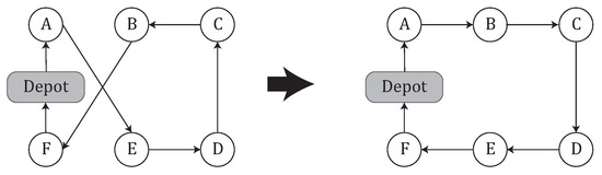
Figure 1.
Example of 2-opt move between B and E nodes, which implies that edges and are removed and edges and are inserted.
1-move: a customer served by a regular route is inserted into a different regular route. Figure 2 shows how customer B is included in a different route. This move produces the neighborhood . The space and time complexity of completely exploring this neighborhood, are and , respectively.
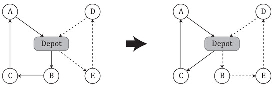
Figure 2.
Example of 1-move of B from solid line route to dashed line route.
Swap-move: a pair of customers served by different regular routes are exchanged. Figure 3 shows the swap of customers B and E. This move produces the neighborhood . The space and time complexity of completely exploring this neighborhood, are and , respectively.
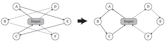
Figure 3.
Example of swap move between B and E nodes.
In-move: a customer served by an occasional driver is included in a regular route. As can be seen in Figure 4 the customer B initially visited by an occasional driver will be served in a regular route after the in-move. This move produces the neighborhood . The space and time complexity of completely exploring this neighborhood, are and , respectively.
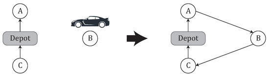
Figure 4.
Example of In-move of B.
Out-move: a customer served by a regular route is assigned to an occasional driver. Figure 5 shows how customer B, initially visited by a regular route, is now served by an occasional driver. This move produces the neighborhood . The space and time complexity of completely exploring this neighborhood, are and , respectively.
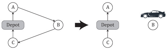
Figure 5.
Example of Out-move of B.
The proposed local search method considers an extended neighborhood formed by the five defined neighborhoods. Algorithm 3 presents the pseudo-code of our proposal. As seen in the algorithm, the method iterates while the current solution is improved (steps 3 to 10). Hence, given an incumbent solution S, the five neighborhoods previously defined are explored in step 4 obtaining , which is the best solution of the extended neighborhood. Then, it is compared with the best solution in step 5, updating if necessary in the following step. If no improvement was made, the guard variable is changed in step 8. At the end, the algorithm returns the local optimum in step 11.
| Algorithm 3 LocalSearch (S) |
|
3.3. Perturbation Procedures
Another important step of the ILS algorithm is the way in which a solution is perturbed or modified. Given that this problem involves routes and occasional drivers assignations, several different perturbations can be explored. Among them, three different perturbation procedures are proposed in this paper, motivated by the need to reach a solution different from the incumbent one and different to its neighbors, considering the neighborhoods previously defined. The proposed perturbation procedures are next described:
RandomMove. A move from the five previously defined neighborhoods is randomly selected and executed, without evaluating the performance impact over the objective function. This perturbation is applied a fixed number of times, defined by the parameter. The complexity of this perturbation method corresponds with the time complexity of the used neighborhood.
RouteCost. This strategy firstly ranks the routes by their cost per customer, and then selects a route according to a probability distribution. The probability of choosing a certain route is given by Equation (1). This approach to select the route to remove is analogous to the one followed in [29] and [30] for the construction phase. In our implementation, removing a route has a time complexity of .
where represents the cost per customer of route , as seen in Equation (2), in which represents the cost of a given route r, and the number of customers attended by a route r. In short, as a proportion, the more costly a route is per customer, the more likely it will be destroyed.
In case that all the customers where removed from a route, the route is deleted. This process is repeated times, producing a number of unassigned customers. Then, those customers are reassigned using the proposed constructive method (see Section 3.1).
RandomDeassign. It randomly selects customers following an uniform distribution, and their assignments are removed from the solution. Then, these customers are reassigned using the constructive method used in the ILS algorithm. In our implementation, removing a random set of customers from a given solution has a time complexity of .
All the three perturbation methods require an input parameter which, for the sake of clarity, we have labeled as . This parameter determines the perturbation size, which has different meaning on each perturbation method, as explained above. Hence, the values analyzed in the experimental experience will be selected accordingly.
3.4. Parallel Cooperation Proposal
The parallel implementation of an algorithm is usually a straightforward task that allows the researcher to make use of the full performance of the computer where the algorithm is run. Moreover, as shown by many works in the literature, parallelism can contribute to the optimization search. For instance, in [31], a parallel Variable Neighborhood Search (VNS) approach is presented, where a cooperation among threads is developed on a master-slave scheme. The authors applied this proposal to successfully solve a well-studied location problem, the p-median problem. Several cooperative schemes for VNS are also studied in [32], showing that cooperation reaches better results than the straightforward parallelization in the obnoxious p-median problem.
Based on the previously exposed ideas, we propose a cooperation scheme for the parallel implementation of the ILS method. This cooperation is shown in Figure 6. As it can be seen, the multi-start ILS execution is divided into N workers, namely to . Each worker will execute independently on a different thread following the implementation shown in Algorithm 1, but applying the cooperation scheme. In particular, each worker creates a solution with the constructive procedure and, then, executes the internal for loop, which corresponds to steps 4 to 10 in the algorithm, labelled as in the figure. After a given number of executions of the loop, a migration of solutions is performed. In this cooperation, each worker with “pushes” (sends) its current best solution to a FIFO queue, , from which the following worker will “pull” (receive) a solution. Notice that sends its solution to , creating a ring topology. Once a solution is taken from the queue, the ILS loop executes on the incoming solution until the following migration or the execution ends.
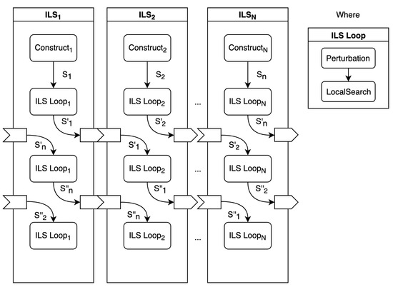
Figure 6.
Parallel cooperation scheme for the ILS based on solution migrations.
The decoupling of workers by means of the queues makes this scheme very flexible, allowing different cooperative structures like master-slave or full connection [32]. However, we propose the ring configuration and the concept of round. A round is completed when a solution has visited every worker once. Therefore, if we set the number of rounds to two, each solution will visit each worker twice. In order to honor the total number of allowed perturbations, the algorithm will divide the number of iterations of the original for loop, given by the np parameter (see step 4 in Algorithm 1) by .
As it will be shown in the next section, the main advantage of this proposal is being able to apply different configurations on each worker. Besides, given that the queues take care of the synchronization of the threads, the execution time will be determined by the slowest worker.
4. Computational Results
This section presents and discusses the computational experience conducted with the algorithms proposed in this paper. Firstly, we describe a set of preliminary experiments that allows us to tune the parameters of the algorithm. Then, we compare the performance of our proposal against the state of the art, which was stated in [16].
In order to perform a fair comparison, we have used the very same set of instances as the previous authors. In particular, they consider six types of instances: types C101 and C201, where customers are clustered; types R101 and R201, where customers are randomly distributed; and types RC101 and RC201, where customers are partially clustered and partially randomly distributed. Following the approach from [16], we generated the different instances among the mentioned six types using the corresponding values for the parameters that characterize each instance. These parameters and their values are the following: the number of occasional drivers, , with ); the compensation rate, , with and for the compensation schemes I and II, respectively; and the flexibility of the occasional drivers, , with . The combination of the values of the parameters across the six types of instances according to [16] produced a total number of 480 instances.
The experiments were run on a machine provided with a Ryzen 7 1700 CPU running at 3 GHz, with 16GB RAM. All the algorithms are implemented in Java 11.
4.1. Preliminary Experimentation
In order to select the best combination of parameters for our proposed algorithms, a representative subset of 70 instances out of a total number of 480 instances, was selected having the following final distribution: 8 instances with , 9 instances with , 26 instances with ; and 27 instances with . The selection was made by randomly picking an instance for each combination of , and .
The first preliminary experiment is devoted to tuning the generation of the initial solution. As stated in Section 3.1, a GRASP approach is proposed. Therefore, it is required to determine the best value of the parameter for this method. Table 1 and Table 2 show the results obtained when solutions are built using the GRASP constructive method and the constructive method coupled with the proposed local search, respectively. In particular, 10,000 constructions are generated in both experiments. The first column of both tables contains the different values of the parameter that have been studied: , where Random means that a value for was randomly selected at each iteration, following a uniform distribution. Besides, the number of times that the algorithm is able to attain the best value is shown in the second column (#B.), being the best value the minimum value found by any of the compared algorithms in each experiment; the third column averages the best costs obtained across the 70 instances (Cost); and, finally, the last column shows the average computation time in seconds (T(s)).

Table 1.
Performance of the different values of for the proposed constructive method after 10,000 iterations.
Table 2.
Performance of the different values of for the proposed constructive method coupled with the local search after 10,000 iterations.
The comparison of Table 1 and Table 2 evidences the contribution of the local search. In a pairwise comparison of rows from both tables, it can be seen that, for each value of , the local search reaches better results not only in the number of times that the best value is obtained, but also in the quality of the solutions (see columns 2 and 3, respectively). Obviously, the CPU time is increased when the local search is run after the constructive process.
Given that the results of and randomly chosen are very similar when the local search is run, both configurations will be selected for the next experiment.
In the following experiment we will assess the contribution of the proposed perturbation methods. To this aim, the perturbations have been run with different values for the perturbation size , for both and randomly chosen. Table 3 shows the results of this experiment, where the first column presents the two values of considered in this experiment; the second column shows the three perturbation procedures, and the third column the values for the parameter. The values for have been determined experimentally taking into account a similar computational effort among the selected values. The remaining columns present the same results as in the previous experiment. To carry out this experimentation, we have run Algorithm 1 after one construction (), which is the same for each instance in all the perturbation methods, hence performing a fair comparison among them. Besides, the value of , which is the number of times the perturbation method is run, was set proportional to the number of occasional drivers. In particular, .
Table 3.
Performance comparison among the proposed perturbation methods.
In view of the values shown in Table 3, it can be seen that the best results are obtained by the RandomMove method with , for both values, and that the influence of the perturbation method over the final score is more important than the value of .
Besides, the RandomDeassign method obtains competitive results, with a difference with respect to the best perturbation configuration, while the RouteCost method obtains the worst results.
Finally, in order to take into account other possible algorithmic strategies, we designed a memetic approach [33] to tackle this problem. Here, the local search was combined with a genetic algorithm where the routes were encoded with a double chromosome for both the regular and the occasional drivers. The usual crossover and mutation operators were also implemented and several configurations were explored in relation with the execution of the local search step.
From those preliminary experiments, we show in Table 4 the results of the most relevant executions of the memetic approach, labeled as MA. In particular, the table shows the comparison of number of best results obtained by the proposal, the exact approach from the state of the art (IP) and the memetic algorithm (MA) on a subset of small-sized instances.
Table 4.
Comparison between , the exact method (IP) and the memetic algorithm (MA).
As it can be seen in the table, the memetic algorithm obtained poor results in relation with the two other proposals, while was able to reach 59 out of the 60 optimal values. In addition, the execution time of MA was more than 50 times longer than the approach. Therefore, we decided to omit the memetic approach from the final comparison.
4.2. Final Comparison
Once the ILS parameters have been studied in the previous section, we now proceed to compare our proposals with the state of the art, whose results will be labelled as . In brief, we propose a multi-start ILS algorithm, namely ; a straightforward parallel version of the multi-start ILS where the iterations of the algorithm are distributed among N threads, called ; and our proposed cooperative parallel ILS with migration of solutions, . This experiment consists on running these algorithms on the whole set of 480 instances. Next, we describe the particular configuration selected for this proposal.
The number of iterations of is 100, which corresponds to 100 constructions generated with , and the perturbation method used was RandomMove with , since this configuration obtained the best results in the previous experimentation. The number of executions of the perturbation method was set to . This configuration is repeated for given that this is a parallel implementation of .
Regarding , we take advantage of the cooperative policy by applying different configurations on each worker. In particular, we have considered to be the number of cores used by the parallel versions of ILS, both and . Therefore, we consider 4 different configurations for . In order to select these configurations we chose the four best configurations in terms of number of best solutions, as shown in Table 3: RandomMove with ( and ), and RandomMove with ( and ). The number of rounds was set to 2, making any solution go through every configuration twice, as explained in Section 3.4.
Table 5 shows the comparison of the proposed ILS algorithms with the state of the art for those instances with 13 and 25 occasional drivers. The results are summarized for each value of , which represents the flexibility of the occasional drivers. For each algorithm (, and ) the averaged cost, the sum of best values (#B.), and the execution time in seconds (T(s)) are calculated. Since no information is given about execution time in [16], only the cost and the number of best results are reported for the SOTA. As it can be seen in the table, all our ILS proposals obtain the best result for all the instances, reaching the same average cost among them and improving the results of SOTA. Regarding the execution time, the fastest algorithm is , which is a straightforward parallel implementation of . is slower than because its execution time is determined by the slowest worker.
Table 5.
Performance comparison for and occasional drivers.
For the medium size instances, where , the results are aggregated by the compensation rate () and the flexibility of the occasional drivers (), as in [16]. Table 6 shows the results with the same indicators as in the small instances, but adding the relative percentage deviation from the best-known value (Gap). Looking at the results, we can point out that the average cost and the number of best results obtained by all the ILS proposals are better than the SOTA. If we focus on the number of best results (#B.), it can be seen that the basic obtains practically the same results than the SOTA in this metric, however, the parallel collaborative scheme, , obtains almost 50% more best results than the SOTA. Furthermore, regarding the gap, it can be seen that all the proposed algorithms obtain better relative deviations from the best-known values than the SOTA, specially the parallel collaborative scheme, (). The execution time follows the same pattern as for the small instances, with being the fastest algorithm and the second one.
Table 6.
Performance comparison for occasional drivers.
Finally, the results for the largest instances with 100 occasional drivers are shown in Table 7 in a similar fashion as the medium-size instances. As it can be seen, the performance gap between the ILS proposals and SOTA widens in terms of the number of best results. In particular, reaches more than twice the number of best results than SOTA, while also improving the average cost and having less than half of the deviation. Note that the other two ILS proposals do not improve the average cost of SOTA by a small margin. However, both ( and ) improve the number of best results obtained. Regarding the average execution time, the results are similar than in the previous tables.
Table 7.
Performance comparison for occasional drivers.
As a first conclusion from the results, we can affirm that the cooperative proposal outperforms the basic , the parallel and the SOTA methods in terms of cost and, specially, in terms of number of best results found. As previously mentioned, the method is slower than as its computation time is limited by the slowest worker. For the sake of space we have omitted the detailed results of all instances. However, we will make them publicly available at http://grafo.etsii.urjc.es/ (accessed on 16 January 2021).
In order to statistically assess the behavior of the algorithms considered in this work, we carried out the Bayesian performance analysis for comparing multiple algorithms over multiple instances simultaneously described in [34,35]. This analysis considers the experimental results as rankings of algorithms, and on the basis of a probability distribution defined on the space of rankings, it computes the expected probability of each algorithm being the best among the compared ones. Not limited to that, it also assesses the uncertainty related to the estimation in the form of credible intervals. These intervals are computed using Bayesian statistics and they estimate the most likely values of the unknown parameter to lie within the interval given a certain probability.
Figure 7 shows the credible intervals (5% and 95% quantiles) and the expected probability of winning for each different implementation of the proposed algorithms and the state-of-the-art method (SOTA) after the joint analysis of the 480 instances. We will refer to the term winning when the algorithm is able to find the best solution in relation to the other methods in the comparison. As seen in the figure, SOTA is the algorithm with least chances for being the winner, with an expected probability of 0.127 of obtaining the best solution. Besides, the probability of and is quite similar (0.243 and 0.276 respectively), with overlapped credible intervals. This result proves that a straightforward parallelization has a small contribution to the quality reached by the algorithm, and the main advantage is the savings in computation time. However, both proposals are better than SOTA since their probabilities of obtaining better solutions than SOTA are higher. Moreover, the expected probability of is the highest, reaching a value of 0.354, showing a credible interval that is not overlapped with any other. In summary, is statistically different from all the other algorithms, and it will reach the best solutions in almost 36% of the instances. The observed length for the intervals in Figure 7 points out that the estimations for SOTA and permit to draw solid conclusions, while for the case of and , due to the overlapping of the intervals, both algorithms have similar probability for being the winners.
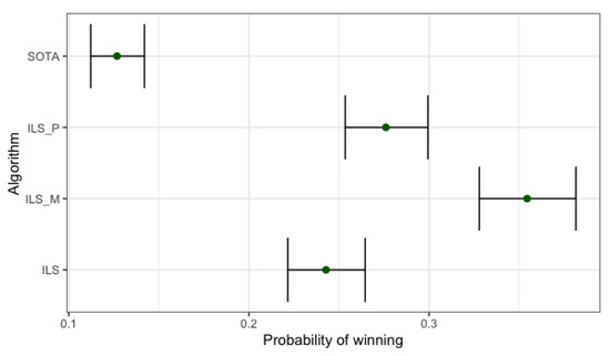
Figure 7.
Credible intervals (5% and 95% quantiles) and expected probability of winning for the proposed Iterated Local Search (ILS) algorithms and the state of the art (SOTA).
Therefore, this statistical analysis proves that, on the one hand, all our ILS proposals obtain better results than the state-of-the-art method and, on the other hand, the proposed cooperative scheme makes a significant difference in relation to the other ILS proposals.
5. Conclusions
Sustainable logistics require the combination of the traditional business logistics and crowd logistics. However, efficient optimization algorithms are required in order to merge these approaches into corporate information systems.
In this work we propose an efficient optimization algorithm based on the Iterated Local Search method which we have assessed on the Vehicle Routing Problem with Occasional Drivers (VRPOD). This problem models realistic situations appearing in the transportation of goods for delivery companies in which crowdshipping, a sustainable means of transport, is feasible, taking into account two different compensation schemes.
In particular, the three proposed implementations of the ILS are able to overcome the results obtained by the state of the art. The ILS design proposed in this paper includes a greedy randomized constructive method to build initial solutions and a local search which explores an extended neighborhood formed by the combination of neighborhoods generated by five different moves. In addition, three perturbation strategies have been proposed for this problem. Moreover, a parallel cooperation scheme has been designed for the ILS proposal. The computational experiments evidence the effectiveness of our algorithm given that it is able to attain all the optimal values when they are known. Besides, it obtains better results than the state-of-the-art method spending a competitive execution time. A statistical assessment of the proposed algorithms performance has been also included, measuring the differences between the ILS methods and the state of the art. In the light of the computational results, we can state that the three different implementations based on the ILS methodology are able to improve the state of the art for the small instances (instances with 13 and 25 occasional drivers) in a few seconds, finding 17 new best-known solutions. A similar behaviour can be observed for the medium-size instances (50 occasional drivers), finding 130 out of 180 new best-known solutions. Finally, in the large instances (those with 100 occasional drivers), the cooperative parallel ILS with solution migrations, , not only reduces the average cost value but also reaches 68 out of 180 new best-known solutions. Furthermore, considering all the three different implementations based on the ILS methodology 115 in total new best-known solutions. To prove the hypothesis that the is the best proposal, a statistical analysis has been included where all the algorithms have been compared. As a conclusion of this analysis, the three different implementations based on the ILS algorithm outperform the state of the art, being the best one among all the studied alternatives.
Therefore, since the previous results are improved by including occasional drivers with our proposal, we can state that our method is able to optimize the last-mile logistics, as recommended in [14]. Hence, since the new routes have smaller costs, the sustainability of the companies is favored. Besides, the reduced computation times of allows the inclusion of our method into corporate information systems.
Future research directions could include different compensation schemes profitable not only for the company but also for the occasional driver, which lead us to a multi-objective optimization problem since both objectives are clearly in conflict. Furthermore, another interesting future line would be to include the possibility of allowing more than one delivery to every occasional driver or even sustainability features included also under a multi-objective approach to show the trade-off among the different objective functions. In addition, the use of more detailed instances with information about the type of vehicles used by the occasional drives will allow to obtain sustainability measures such as the carbon footprint of a route. Finally, in order to study more realistic scenarios, new instances with stochastic modeling of the demand or the travelling times could be defined, as suggested in [36]. Of course, adding new features to the considered problem would lead us to adapt the ILS methodology and check the robustness of our algorithm since new constraints are incorporated.
Author Contributions
Conceptualization, R.M.-S., A.D.L.-S. and J.M.C.; Data curation, R.M.-S., A.D.L.-S. and J.M.C.; Formal analysis, A.D.L.-S.; Funding acquisition, M.L.D.-J.; Methodology, R.M.-S., A.D.L.-S. and J.M.C.; Project administration, M.L.D.-J.; Software, R.M.-S. and J.M.C.; Supervision, J.M.C.; Writing—original draft, R.M.-S., A.D.L.-S. and J.M.C.; Writing—review & editing, R.M.-S., A.D.L.-S., M.L.D.-J. and J.M.C. All authors have read and agreed to the published version of the manuscript.
Funding
This work has been partially supported by the Spanish Ministerio de Ciencia, Innovación y Universidades (MCIU/AEI/FEDER, UE) under grant ref. PGC2018-095322-B-C2; Comunidad de Madrid y Fondos Estructurales de la Unión Europea under grant ref. S2018/TCS-4566 and the Junta de Andalucía, FEDER-UPO Research & Development Call, under grant ref. UPO-1263769.
Institutional Review Board Statement
Not applicable.
Informed Consent Statement
Not applicable.
Data Availability Statement
Detailed results and instances will be publicly available at http://grafo.etsii.urjc.es/ (accessed on 16 January 2021).
Acknowledgments
The authors wish to express their gratitude to C. Archetti, M. Savelsbergh and G. Speranza for their collaboration in the provision of all their previous results.
Conflicts of Interest
The authors declare no conflict of interest.
References
- Allen, J.; Piecyk, M.; Piotrowska, M.; McLeod, F.; Cherrett, T.; Ghali, K.; Nguyen, T.; Bektas, T.; Bates, O.; Friday, A.; et al. Understanding the impact of e-commerce on last-mile light goods vehicle activity in urban areas: The case of London. Transp. Res. Part Transp. Environ. 2018, 61, 325–338. [Google Scholar] [CrossRef]
- Jia, Y.H.; Chen, W.N.; Gu, T.; Zhang, H.; Yuan, H.; Lin, Y.; Yu, W.J.; Zhang, J. A dynamic logistic dispatching system with set-based particle swarm optimization. IEEE Trans. Syst. Man Cybern. Syst. 2017, 48, 1607–1621. [Google Scholar] [CrossRef]
- Qin, G.; Tao, F.; Li, L. A vehicle routing optimization problem for cold chain logistics considering customer satisfaction and carbon emissions. Int. J. Environ. Res. Public Health 2019, 16, 576. [Google Scholar] [CrossRef]
- Gevaers, R.; Van de Voorde, E.; Vanelslander, T. Characteristics of innovations in last-mile logistics-using best practices, case studies and making the link with green and sustainable logistics. Assoc. Eur. Transp. Contrib. 2009, 1–21. [Google Scholar]
- Sampaio, A.; Savelsbergh, M.; Veelenturf, L.; Van Woensel, T. Chapter 15: Crowd-Based City Logistics. In Sustainable Transportation and Smart Logistics; Faulin, J., Grasman, S.E., Juan, A.A., Hirsch, P., Eds.; Elsevier: Amsterdam, The Netherlands, 2019; pp. 381–400. [Google Scholar]
- Carbone, V.; Rouquet, A.; Roussat, C. The Rise of Crowd Logistics: A New Way to Co-Create Logistics Value. J. Bus. Logist. 2017, 38, 238–252. [Google Scholar] [CrossRef]
- Devari, A.; Nikolaev, A.G.; He, Q. Crowdsourcing the last mile delivery of online orders by exploiting the social networks of retail store customers. Transp. Res. Part Logist. Transp. Rev. 2017, 105, 105–122. [Google Scholar] [CrossRef]
- Botsman, R. Crowdshipping: Using the crowd to transform delivery. AFR Boss Mag. 2014. [Google Scholar]
- Mckinnon, A. Crowdshipping: A Communal Approach to Reducing Urban Traffic Levels? 2016. Available online: https://www.alanmckinnon.co.uk/story_layout.html?IDX=714&b=56 (accessed on 6 January 2021).
- Guo, X.; Jaramillo, Y.J.L.; Bloemhof-Ruwaard, J.; Claassen, G. On integrating crowdsourced delivery in last-mile logistics: A simulation study to quantify its feasibility. J. Clean. Prod. 2019, 241, 118365. [Google Scholar] [CrossRef]
- Simoni, M.D.; Marcucci, E.; Gatta, V.; Claudel, C.G. Potential last-mile impacts of crowdshipping services: A simulation-based evaluation. Transportation 2020, 47, 1933–1954. [Google Scholar] [CrossRef]
- Toth, P.; Vigo, D. Vehicle Routing: Problems, Methods, and Applications; SIAM: Philadelphia, PA, USA, 2014. [Google Scholar]
- Braekers, K.; Ramaekers, K.; Van Nieuwenhuyse, I. The vehicle routing problem: State of the art classification and review. Comput. Ind. Eng. 2016, 99, 300–313. [Google Scholar] [CrossRef]
- Ranieri, L.; Digiesi, S.; Silvestri, B.; Roccotelli, M. A review of last mile logistics innovations in an externalities cost reduction vision. Sustainability 2018, 10, 782. [Google Scholar] [CrossRef]
- Wang, Y.; Zhang, D.; Liu, Q.; Shen, F.; Lee, L.H. Towards enhancing the last-mile delivery: An effective crowd-tasking model with scalable solutions. Transp. Res. Part Logist. Transp. Rev. 2016, 93, 279–293. [Google Scholar] [CrossRef]
- Archetti, C.; Savelsbergh, M.; Speranza, M.G. The Vehicle Routing Problem with Occasional Drivers. Eur. J. Oper. Res. 2016, 254, 472–480. [Google Scholar] [CrossRef]
- Dahle, L.; Andersson, H.; Christiansen, M. The Vehicle Routing Problem with Dynamic Occasional Drivers; Computational Logistics; Bektaş, T., Coniglio, S., Martinez-Sykora, A., Voß, S., Eds.; Springer International Publishing: Cham, Switzerland, 2017; pp. 49–63. [Google Scholar]
- Macrina, G.; Di Puglia Pugliese, L.; Guerriero, F.; Laganà, D. The Vehicle Routing Problem with Occasional Drivers and Time Windows. In Optimization and Decision Science: Methodologies and Applications; Sforza, A., Sterle, C., Eds.; Springer International Publishing: Cham, Switzerland, 2017; pp. 577–587. [Google Scholar]
- Gdowska, K.; Viana, A.; Pedroso, J.P. Stochastic last-mile delivery with crowdshipping. Transp. Res. Procedia 2018, 30, 90–100. [Google Scholar] [CrossRef]
- Arslan, A.M.; Agatz, N.; Kroon, L.; Zuidwijk, R. Crowdsourced Delivery: A Dynamic Pickup and Delivery Problem with Ad-Hoc Drivers. Transp. Sci. 2019, 53, 222–235. [Google Scholar] [CrossRef]
- Behrend, M.; Meisel, F.; Fagerholt, K.; Andersson, H. An exact solution method for the capacitated item-sharing and crowdshipping problem. Eur. J. Oper. Res. 2019, 279, 589–604. [Google Scholar] [CrossRef]
- Brandão, J. A deterministic iterated local search algorithm for the vehicle routing problem with backhauls. TOP 2016, 24, 445–465. [Google Scholar] [CrossRef]
- Cattaruzza, D.; Absi, N.; Feillet, D.; Vigo, D. An iterated local search for the multi-commodity multi-trip vehicle routing problem with time windows. Comput. Oper. Res. 2014, 51, 257–267. [Google Scholar] [CrossRef]
- Silva, M.M.; Subramanian, A.; Ochi, L.S. An iterated local search heuristic for the split delivery vehicle routing problem. Comput. Oper. Res. 2015, 53, 234–249. [Google Scholar] [CrossRef]
- Lourenço, H.R.; Martin, O.C.; Stützle, T. Iterated Local Search. In Handbook of Metaheuristics; Glover, F., Kochenberger, G.A., Eds.; Springer: Boston, MA, USA, 2003; pp. 320–353. [Google Scholar]
- Feo, T.A.; Resende, M.G.C. A probabilistic heuristic for a computationally difficult set covering problem. Oper. Res. Lett. 1989, 8, 67–71. [Google Scholar] [CrossRef]
- Feo, T.A.; Resende, M.G.C.; Smith, S.H. A Greedy Randomized Adaptive Search Procedure for Maximum Independent Set. Oper. Res. 1994, 42, 860–878. [Google Scholar] [CrossRef]
- Croes, G.A. A Method for Solving Traveling-Salesman Problems. Oper. Res. 1958, 6, 791–812. [Google Scholar] [CrossRef]
- Faulin, J.; Juan, A.A. The ALGACEA-1 method for the capacitated vehicle routing problem. Int. Trans. Oper. Res. 2008, 15, 599–621. [Google Scholar] [CrossRef]
- Buxey, G.M. The Vehicle Scheduling Problem and Monte Carlo Simulation. J. Oper. Res. Soc. 1979, 30, 563–573. [Google Scholar] [CrossRef]
- Crainic, T.; Gendreau, M.; Hansen, P.; Mladenovic, N. Cooperative Parallel Variable Neighborhood Search for the p-Median. J. Heuristics 2004, 10, 293–314. [Google Scholar] [CrossRef]
- Herrán, A.; Colmenar, J.M.; Martí, R.; Duarte, A. A parallel variable neighborhood search approach for the obnoxious p-median problem. Int. Trans. Oper. Res. 2020, 27, 336–360. [Google Scholar] [CrossRef]
- Neri, F.; Cotta, C.; Moscato, P. Handbook of Memetic Algorithms; Springer: Cham, Switzerland, 2011. [Google Scholar]
- Calvo, B.; Ceberio, J.; Lozano, J.A. Bayesian Inference for Algorithm Ranking Analysis. In Proceedings of the Genetic and Evolutionary Computation Conference Companion; ACM: New York, NY, USA, 2018; pp. 324–325. [Google Scholar]
- Calvo, B.; Shir, O.M.; Ceberio, J.; Doerr, C.; Wang, H.; Bäck, T.; Lozano, J.A. Bayesian Performance Analysis for Black-box Optimization Benchmarking. In Proceedings of the Genetic and Evolutionary Computation Conference Companion; ACM: New York, NY, USA, 2019; pp. 1789–1797. [Google Scholar]
- Juan, A.A.; David Kelton, W.; Currie, C.S.M.; Faulin, J. Simheuristics Applications: Dealing With Uncertainty In Logistics, Transportation, and Other Supply Chain Areas. In Proceedings of the 2018 Winter Simulation Conference (WSC), Gothenburg, Sweden, 9–12 December 2018; pp. 3048–3059. [Google Scholar]
Publisher’s Note: MDPI stays neutral with regard to jurisdictional claims in published maps and institutional affiliations. |
© 2021 by the authors. Licensee MDPI, Basel, Switzerland. This article is an open access article distributed under the terms and conditions of the Creative Commons Attribution (CC BY) license (http://creativecommons.org/licenses/by/4.0/).