Article

Stochastic Chebyshev Goal Programming Mixed Integer Linear Model for Sustainable Global Production Planning

by
Chia-Nan Wang
1,*,
Nhat-Luong Nhieu
1,* and
Trang Thi Thu Tran
2
1
Department of Industrial Engineering and Management, National Kaohsiung University of Science and Technology, Kaohsiung 80778, Taiwan
2
Department of Industrial Engineering and Engineering Management, National Tsing Hua University, Hsinchu 300044, Taiwan
*
Authors to whom correspondence should be addressed.
Mathematics 2021, 9(5), 483; https://doi.org/10.3390/math9050483
Submission received: 5 February 2021 / Revised: 19 February 2021 / Accepted: 22 February 2021 / Published: 26 February 2021
(This article belongs to the Special Issue Statistical Methods in Economics)

Abstract

:
Production planning is a necessary process that directly affects the efficiency of production systems in most industries. The complexity of the current production planning problem depends on increased options in production, uncertainties in demand and production resources. In this study, a stochastic multi-objective mixed-integer optimization model is developed to ensure production efficiency in uncertainty conditions and satisfy the requirements of sustainable development. The efficiency of the production system is ensured through objective functions that optimize backorder quantity, machine uptime and customer satisfaction. The other three objective functions of the proposed model are related to optimization of profits, emissions, and employment changing. The objective functions respectively represent the three elements of sustainable development: economy, environment, and sociality. The proposed model also assures the production manager’s discretion over whether or not to adopt production options such as backorder, overtime, and employment of temporary workers. At the same time, the resource limits of the above options can also be adjusted according to the situation of each production facility via the model’s parameters. The solutions that compromise the above objective functions are determined with the Chebyshev goal programming approach together with the weights of the goals. The model is applied to the multinational production system of a Southeast Asian supplier in the textile industry. The goal programming solution of the model shows an improvement in many aspects compared to this supplier’s manufacturing practices under the same production conditions. Last but not least, the study develops different scenarios based on different random distributions of uncertainty demand and different weights between the objective functions. The analysis and evaluation of these scenarios provide a reference basis for managers to adjust the production system in different situations. Analysis of uncertain demand with more complex random distributions as well as making predictions about the effectiveness of scenarios through the advantages of machine learning can be considered in future studies.

1. Introduction

The textile industry plays a vital role in many Asian countries’ economies especially in emerging nations. It is a diverse sector, which has its own chain that includes converting chemical or natural fibers into consumer goods such as garments or industrial textiles. It will require force to transfer from the existing Industry 3.0 to Industry 4.0 and empower smart production. Sustainable fabrication is significant for the effective use of waste reduction, resources allocation efficiency and related costs. Textiles are severely interlinked with environmental, governance and social issues. In the past, efforts of the manufacturer have been primarily concentrated on enhancing the social attributes of textiles, such as creating suitable working conditions, setting minimum wages, maintaining work safety, etc. However, over the years, concern about the textile’s industry’s environmental impacts have been risen especially regarding greenhouse gas (GHG) emissions which may arise from washing (using water heating and detergents), processing fossil fuels into synthetic fibers and dyeing textiles. This industry is one of the major sources of GHG emissions because of its fabrication technologies and transportation [1].
Presently, it is not only faced with a global aggressive manufacturing environment, but also incessant rising demand. Therefore, the textile industry needs to optimize its manufacturing operations to enhance productivity, customization, and product quality, and minimize lead times [2]. Indeed, these factors have led manufacturers to apply planning strategies that make manufacturing procedure more effective, and encouraging, and improve production structures [3]. These have driven textile and clothing supply chains to optimize their production planning to satisfy the challenges demanded by the market. Global production planning ascertains the production capacity to meet the de-mand, in which design configurations and production scenarios are evaluated that require a combination of factors, which are the maximization of profit, machine operation time, and customer satisfaction level, and the minimization of costs, emissions, and workforce changing at once.
As a theoretical contribution of this study, the proposed mixed-integer programming model integrates all typical production options such as regular production, production using temporary workers, overtime and backorder. Moreover, the production-planning problem that this model deals with has characteristics of globalization, which is reflected in a multi-product, multi-period, multi-country production system and an uncertain production environment. Another novelty of the model is the set of objective functions that ensures that the production system satisfies the requirements of the new production era to be efficient and sustainable. The objective functions towards sustainability include optimization of profits, emissions and changes in employment. Meanwhile, optimization of backorders, machine use, and customer satisfaction are the target functions that ensure efficiency. The compromise solution of the above objective functions is achieved through the Chebyshev variant of goal programming. This variation is believed to be able to avoid extreme solutions that can be encountered with lexicographic goal programming. Finally, as a practical contribution, a set of scenarios is developed regarding two factors: uncertainty of demand and the weight of objective functions. Evaluation of these scenarios provides production managers with predictions for the refinement of production systems when the two factors mentioned above change.
The paper is organized as follows. Section 2 reviews the literature and related studies. The mathematical multi-objective mixed-integer programming model is presented in Section 3. Section 4 proposes a result from an empirical study for validation with its optimization approaches. Section 5 concludes the paper, and further work of this study.

2. Literature Review

The production-planning process is seen as the process of finding a way that economically or efficiently uses resources required for production such as manpower, materials, and equipment. In other words, the typical decisions in production planning are affected by trade-offs between financial and productivity efficiency objectives. In particular, financial targets are mainly related to increasing profits or reducing costs, including production costs, labor costs, material costs, inventory costs, and so on. In terms of production efficiency, production planning should consider the ability to supply products as well as the effects of other factors during operation such as overtime, inventory level, and backorders. For long-medium, or short-term periods, the production plan is classified into a strategic plan, a tactical plan, and an operational plan, respectively. The objective of strategic plans is to sustain growth and create a competitive advantage. Meanwhile, tactical and operational plans make decisions about product flow, manpower, and machine capacity with more detailed information to create economic and productivity efficiency [4].
Quantitative models and methods are supposed to assist operations managers with grasping the complexity of the production system and the decisions associated with it [5]. Production plans can be developed with forecasted demand using DEA-based approaches, which were proposed by Du et al. [6]. In that study, the production system performance is measured by the CCR efficiency score, which was introduced by Charnes, Cooper and Rhodes [7]. Another heuristic-based approach is recommended to determine the effective inventory level to save inventory-related costs, such as holding cost and backorder penalty [8]. The results of the synthesis paper published in 2019 by Bagshaw stated that different quantitative models are developed for different production conditions and problem characteristics [9]. In other words, a universal model or method for all operational production problems does not exist. This study also demonstrates that linear programming planning being an effective quantitative analysis approach for the improvement of production systems [9,10]. An optimal control formulation, introduced by Devizón et. al., integrates two dynamical systems with typical inventory process parameters such as production rate, inventory level, and costs [11]. Another linear planning model developed to minimize costs in the mining industry is suggested by Ozsan et al. The solution of this model is under different production conditions due to limitations on resources [12]. In research published in 2018, Campo developed an optimized mathematical model for the whole production planning problem with the objective function and constraints that represent the nature of the garment industry. In which, the model includes variables that affect specific production systems of the garment industry such as physical variations of fabrics, skills of new workers, and so on [3]. For the furniture industry, Gremani’s mathematical model solves the problem of the trade-off between inventory and production of semi-finished or finished products. The results of the study show that while inventory of semi-finished or chopped materials is more cost-effective, it is advantageous to determine the quantity of finished product inventory [13]. The special requirements for their highly skilled workforce and long-time flexibility are characteristic elements of the automotive industry, according to Sillekens et al. Therefore, the workforce planning has been integrated into the mathematical model that incorporates a heuristic algorithm to make useful decisions for automotive production planning [14]. Another application of linear programming model in production planning is in the food industry. The mathematical model of Munhoz and Morabito is concerned with the acidity parameters of the product that are typical of the fruit juice production process [15].
The review paper by Ali Cheraghalikhani, Farid Khoshalhan, and Hadi Mokhtari has categorized production planning models into 6 groups, as showen in Table 1 [16]. Accordingly, the group 1 and group 2 models solve the problem of production planning under certain conditions. Meanwhile, the studies of the remaining groups have considered the uncertainties when developing models or optimization algorithms. While group 3 and group 4 approach uncertainty solutions using fuzzy theory, the studies in group 5 and group 6 apply the theories and probability distributions. This study also pointed out important issues in the production planning problem where the number of related studies decreased over time. Machine utilization, labor characteristics, and multiple facilities are the issues on the list. In the conclusion of this review, the authors propose potential research directions for the production planning problem. Among them, there are multi-objective stochastic models with more than three important issues considered.
According to research by Mula et al., uncertainty factors in the production system are listed as demand, environment, system resource, lead time, and yield. The study also synthesizes common approaches to uncertainty including stochastics model, dynamic programming, fuzzy theory, and simulation-based approaches [17].
Uncertainty in production plans often appears as demand uncertainty or fluctuations in the production process, such as production times or material loss. Bakir and Byrne analyzed the difference of the solutions provided by deterministic model and stochastic model, in which the uncertainty factor is market demand. The analytical results show that this difference is dependent on the variance of uncertain demand [18].
The uncertainty of parameters in the linear planning model is also approached in terms of fuzzy numbers. Accordingly, some of the parameters describing the production system limit are recognized by the authors as uncertain and described as fuzzy parameters [19,20,21]. In addition, parameters intended to determine the value of the target functions such as purchasing materials cost or production cost, can also be uncertain. Therefore, the linear programming model in Vasant’s study in 2006 also introduced a fuzzy objective function [22]. In a recently published study, the authors used fuzzy numbers to describe the uncertainty of unit production time, inventory time, and packing time in the automotive industry. The results of the linear planning model are assessed to have improved the production system in terms of shortening inventory times as well as increasing economic efficiency [23]. Zimerman’s method has been applied in the fuzzy mathematical linear programming model, which minimizes all kinds of costs by Kalaf et al. [24]. Baykasoglu and Gocken converted the fuzzy numbers to a non-linear crisp equivalent before using a Tabu Search algorithm to find an optimized solution [25]. Meanwhile, another choice is a genetic algorithm for solving the crisp model. Moreover, this study also uses a combination of fuzzy AHP and Topis to determine the solution that is reconciled [26,27].
In addition to the fuzzy number approaches, production planning uncertainty is also examined through stochastic models with random distributions and the theory of probability. Orcun presented an integrated non-linear programming model with uncertain demand. The author then used a heuristics approach to evaluate the trade-off between the production system’s time and safety stock level [28]. A hybrid programming model is developed through a combination of stochastic programming and linear programming for the refinery’s production plan, in which the weighting factor is used to control the uncertainty of the hybrid model [29]. Kazemi Zanjani used a scenario tree to control demand uncertainty in a multi-product production planning study. The scenarios in this stochastic model are defined based on the probability distribution of demand during production planning [30]. With similar approaches, Zhang created scenarios for demand uncertainty based on optimistic, pessimistic, and neutral forecast values and their probabilities [31]. For the probabilities, Kazemi Zanjani uses the mean values of the uncertainty parameters as a method for processing the proposed stochastic model [32].
As mentioned above, production plans not only target financial and economic benefits but also consider objectives such as employment, production time, etc. Consequently, the presence of studies that place more than one objective function in a linear programming model is growing. Komsiyah’s research has proposed a multi-objective model with the fuzzy goal programming approach in the furniture industry. However, the objective functions of this model revolve around different cost categories that can be combined into a total cost objective function [33]. Meanwhile, in addition to costs, Tirkolaee’s study has pointed out another objective function, which is to maximize customer satisfaction. In that study, the authors applied weighted goal programming to solve the problem of multi-objective production planning with assumptions that did not consider overtime and outsourcing [34]. A study applied in Hong Kong has developed an optimization model with three target functions: Maximizing profit, minimizing costs due to defective products, and maximizing equipment utilization at a certain production facility [35]. A similar study has been developed for multinational production systems in which ensuring stability in employment and optimizing the efficiency of the import/export quota becomes the objective functions of the mathematical model [36].
In recent years, the impact of climate change on social activities has become more and more apparent. In particular, industry and manufacturing are often considered the source that generates more emissions compared to other sectors. Therefore, environmental factors also appear in the optimization models to help managers make sustainable production decisions. These environmental impacts in the manufacturing sector are often considered by researchers in terms of production energy consumption. In 2018, Hahn and Brandenburg proposed an optimization model in which the environmental impact factors are converted into a form of costs [37]. Taking a similar approach, Tsai’s model describes the environmental impacts such as carbon taxes and the cost savings from reused energy [38]. The optimization model of Modarres and Izadpanahi published in 2016 has the relationship between the uncertainty level of the parameters and the value of the cost of electrical energy. Goal programming is again chosen as the approach to solve the multi-objective model of production planning [39]. In order to increase the efficiency of planning processes, optimization models and algorithms are increasingly integrated both quantitatively and extensively with project management tools [40]. Research by Valenko and Klanšek presented an integrated approach to optimization and Microsoft Project software that increased the cost-effectiveness of the planning process [41].
In summary, the effectiveness of decisions in the production planning process is supported by the results of numerous studies with different approaches. The approach that uses optimization mathematical models has been showing useful applications in the global production planning problems of many industries. Regarding production options, a few studies consider overtime, backorder or part-time worker production in addition to regular production. For the model’s objective functions, most studies focus on economic factors such as profits, costs, and penalties. Meanwhile, studies in recent years consider the environmental impact of production systems as an objective function. In addition, indicators showing the system performance such as maximizing utilization of equipment and customer satisfaction are also considered in the models. Moreover, the uncertainty of the parameters in the model has also shown to have a significant effect on the optimization results by researchers. As the results summarize in Table A1, this study develops a model that integrates the above factors simultaneously.

3. Methodology

3.1. Sets, Parameters and Decision Variables

In this optimization models, parameters and decision variables are formulated based on the set of product families, manufacturing facilities, the time period and the objective function as Table 2.
As shown in Table 3, the model parameters can be classified as five groups. The first group is the parameters related to the selling price of the product along with the costs in production, labor, inventory, backorder penalties, recruitment and layoffs. The second parameter group describes the upper and lower boundaries of inventory, backorder, workforce, and machine capacity. The third group includes parameters related to demand, the standard deviation of demand and its probability under uncertainty. The parameters that provide information about the processing time of product families by the machine and the operator are classified in the fourth group. The fifth group includes the parameters of total worker time, overtime limits and allowable rates of workforce change in production facilities. In addition, such parameters as batch size, production specific electricity use of product families; emission factor of manufacturing facilities; goal value, and weight of objective functions fall into this group.
The decision variables of the model assist managers in the optimal quantity of products that can be sold, S i t , based on information about demand under uncertain conditions. In Table 4, the above production quantities supplied by sources including regular production, temporary worker production, overtime production, inventory, and backorder are denoted x i j t , y i j t ,   v i j t , I i j t , B i j t respectively. In addition, the model also makes decisions about the workforce level ( W j t ) as well as the amount of recruitment ( H j t ) and layoffs ( F j t ) in manufacturing facilities in each period. Furthermore, the total overtime ( O T j t ), temporary labor use time ( T P T j t ), and machine uptime ( M P T j t ) are also calculated by the model. Finally, deviation variables ( o k and u k ) are used to determine the difference between the goal value and the achieved value of the objective functions obtained by the solution. The maximal deviation, ω, is used for Chebyshev Goal Programming to ensure balance between objective functions.

3.2. Model Formulation

3.2.1. Objective Functions

In this paper, the authors aim for six objective functions that reflect the efficiency of the production system in both economic aspects and factors of sustainable development such as environment and society. First, this model maximizes the profitability of the production system (VND). In Equation (1), the first term represents the estimated total revenue while the rest shows the costs. Those costs are production costs, labor costs, inventory costs, backorder penalties, and cost of hiring/firing workers are presented in the order. The second object function of this model is to minimize emissions (tCO2) that are estimated based on parameters such as emission factor and specific electricity use for production as Equation (2).
M a x i m i z e   i t P i . S i t ( i j t ( PC ij F . x i j t + PC ij T . y i j t + OTC ij . v i j t ) . B Z i ) ( j t LC j F . W j t + LC j T . T P T j t + LC j OT . O T j t )   i j t IC ij . I i j t . B Z i     i j t B O C ij . B i j t . B Z i ( j t HC j . H j t + F C j . F j t )
M i n i m i z e   i j t ( x i j t + y i j t + v i j t ) . B Z i . E F j . SE )
Besides environmental impacts, social influences are also a part of ensuring sustainable development. In Equation (3), this study aims to minimize changes in the workforce level (man). This objective function both ensures production stability through ensuring the skill of workers, while also minimizing employment disturbances in the area where the manufacturing facilities are located.
M i n i m i z e   j t ( H j t + F j t )
Backorder is one of the production planning options that this model considers. Although this option can bring some advantages to the production system such as saving inventory space, a large backorder could lead to the risk of customers turning to alternative suppliers. Therefore, as Equation (4), the next objective function is to minimize the amount of system production backorder (unit).
M i n i m i z e   i j t B i j t . B Z i
In order to improve the efficiency of investment by increasing the utilization rate of production machines, the model maximizes the total operating time of production machinery (hour) in all manufacturing facilities through Equation (5).
M a x i m i z e   j t M P T j t
In Equation (6), the model’s sixth objective function is to maximize customer satisfaction level (%), which is determined by the ratio between the amount of product the system can supply and the expected value of demand. This higher ratio can improve the popularity of the product in the market, but it can also increase costs, leading to a decrease in net profit.
M a z i m i z e   i ( t S i t P r m i n D i t m i n +   P r m o s t D i t m o s t + P r m a x D i t m a x ) T . I

3.2.2. Constraints

The constraints presented in this section describe the resource limitation and policy of the production system. In Equations (7) and (8), the quantity of products expected to be sold does not exceed the expected value of demand and is above the minimum known demand. The expected values of demand are estimated through known minimum, most-likely, and forecasted maximum demand, combined with their probabilities. This expected sales quantity is balanced with regular production, overtime production, production by temporary workers, inventory, and backorder, as shown in Equation (9). The binary decision variable φ i j t in Equation (10) is used to determine the minimum inventory level in Equation (11). The right-hand side of Equation (11) describes the safety stock of a product if it is regularly produced at a given facility over a certain period of time with service level type II (β). In which, z β is the inverse distribution function of a standard normal distribution with cumulative probability β [42]. Equations (12) and (13) ensure that inventory level and backorder do not exceed the maximum allowed limit.
S i t P r m i n D i t m i n +   P r m o s t D i t m o s t + P r m a x D i t m a x i I , t T
S i t D i t m i n   i I , t T
j ( I i j t 1 B i j t 1 + x i j t + y i j t + v i j t I i j t + B i j t ) . B Z i =   S i t i I , t T
{ x i j t φ i j t . B i g M x i j t φ i j t i I , j J , t T
I i j t . B Z i   φ i j t . z β . ( P r m i n σ i m i n +   P r m o s t σ i m o s t + P r m a x σ i m a x ) i I , j J , t T
i I i j t . B Z i   I L j t j J , t T
j B i j t . B Z i   B O L i t i I , t T
Equation (14) defines change in the workforce by recruiting new workers and layoffs. In particular, the number of workers at a time cannot be outside the upper and lower borders according to the policies of each manufacturing facility as Equation (15). Moreover, Equations (16) and (17) ensure that the number of newly recruited or fired workers cannot exceed a permitted percentage compared to the workforce level in the preceding period. Equation (18) is a non-linear variation of the equation H j t . F j t = 0 , which ensures that manufacturing facilities cannot hire and fire workers in the same period.
W j t =   W j t 1 +   H j t   F j t j J , t T
W j m i n W j t W j m a x j J , t T
H j t WLC j . W j t 1 j J , t T
F j t   WLC j . W j t 1 j J , t T
{ H j t   θ j t . B i g M F j t ( 1 θ j t ) . B i g M j J , t T
The constraints (19) ensure that the total time required for regular production does not exceed the total time of the workforce. Similarly, constraints (20)–(23) represent the limits of the production time by temporary workers and overtime. In Equations (24) and (25), the total time required for the aforementioned production types is also limited by the design capacity of the machinery system at the production facility. Finally, all decision variables in this model are considered as non-negative variables.
i PT i F . x i j t . B Z i   δ j . W j t j J , t T
i PT i T . y i j t . B Z i   T P T j t j J , t T
i PT i F . v i j t . B Z i   O T j t j J , t T
T P T j t T P L j t j J , t T
O T j t     δ j . α j . W j t j J , t T
i MT i F x i j t + i MT i T y i j t +   i MT i F z i j t M P T j t j J , t T
M P T j t M L j t j J , t T

3.3. Chebyshev Goal Programming (CGP) Application

In order to find compromise solutions for all six objective functions outlined above, this study uses the Chebyshev goal programming approach, also known as Minmax Goal Programming. The difference of this variant compared to other variants of goal programming such as weighted goal programming or lexicographic goal programming is to assist in finding balanced solutions between the objective functions instead of extreme solutions. In the first step of this approach, the goal values of the objective functions G k are set either through solving the optimization problem for each objective function individually or consulting decision makers. Next, the deviation variables in both negative u k and positive o k directions from the goal value of each objective function are added. The result of the above step is to form new constraints of the model that are presented in Equations (26)–(31).
i t P i . S i t ( i j t ( PC ij F . x i j t + PC ij T . y i j t + OTC ij . v i j t ) . B Z i )   ( j t LC j F . W j t + LC j T . T P T j t + LC j OT . O T j t )       i j t IC ij . I i j t . B Z i   i j t B O C ij . B i j t . B Z i   ( j t HC j . H j t + F C j . F j t ) +   u 1 o 1 =   G 1  
i j t ( x i j t + y i j t + v i j t ) . B Z i . E F j . SE ) +   u 2 o 2 =   G 2
j t ( H j t + F j t )   +   u 3 o 3 =   G 3
i j t B i j t . B Z i +   u 4 o 4 =   G 4
j t M P T j t +   u 5 o 5 =   G 5
i ( t S i t P r m i n D i t m i n +   P r m o s t D i t m o s t + P r m a x D i t m a x ) T . I +   u 6 o 6 =   G 6
( u 1 G 1 ) .   W E 1   ω
( o 2 G 1 ) .   W E 2   ω
( o 3 G 1 ) .   W E 3   ω
( o 4 G 1 ) .   W E 4   ω
( u 5 G 1 ) .   W E 5   ω
( u 6 G 1 ) .   W E 6   ω
The goal values are then used as a normalized constant according to the percentage normalization method to convert the deviation variables to the same unit. Additionally, each deviation variable of each objective function has a weighting parameter W E k that represents its importance relative to the rest. These deviation variables are controlled by the maximal deviation variable ω as constraints (32)–(37). Finally, the only objective function of the model is to minimize the maximum deviation variable with Equation (38).
M i n i m i z e     ω

4. Results

4.1. Case Study of Textile Industry

In this study, a multiple objective optimization model was developed, which applies for the multinational textile supplier’s production planning process. Their production system consists of two manufacturing facilities in Vietnam (VN-1, VN-2) and another in Cambodia (KH). These facilities employ an average of 500 full-time employees to produce five product families including large-sized handbags (LH), handbags (HB), backpacks (BP), wallets (W), and key bags (KB) with a total production in 2019 of approximately one million products as presented in Figure 1. According to production managers, the average required production time of the above product families for temporary and full-time workers is different as described in Figure 2.
In Table 5, manufacturing facilities have the same total number of periodic working hours, but different labor policies such as allowable rate of the workforce changing, upper/lower limits of workforce level, maximum inventory level, overtime limit, and machine capacity.
To estimate the production system emissions, this study is based on the textile industry’s average electrical energy consumption [43] and the emissions factor of the country in which the products are manufactured [44]. Under uncertain conditions, the expected value of demand for product families is estimated using the three-point estimation technique with the program evaluation and review technique (PERT) distribution. Accordingly, the probabilities for the known minimum, most-likely and forecasted maximum demand are 1/6, 4/6, and 1/6 respectively. The optimization problem is solved through IBM CPLEX software version 12.8 on hardware CPU i7 intel and 16 GB RAM. Table 6 describes the dimensions of the optimization problem. By solving the model with each objective function individually, the extreme solutions and their CPU times form the payoff matrix as Table 7.

4.2. Goal Programming Solution
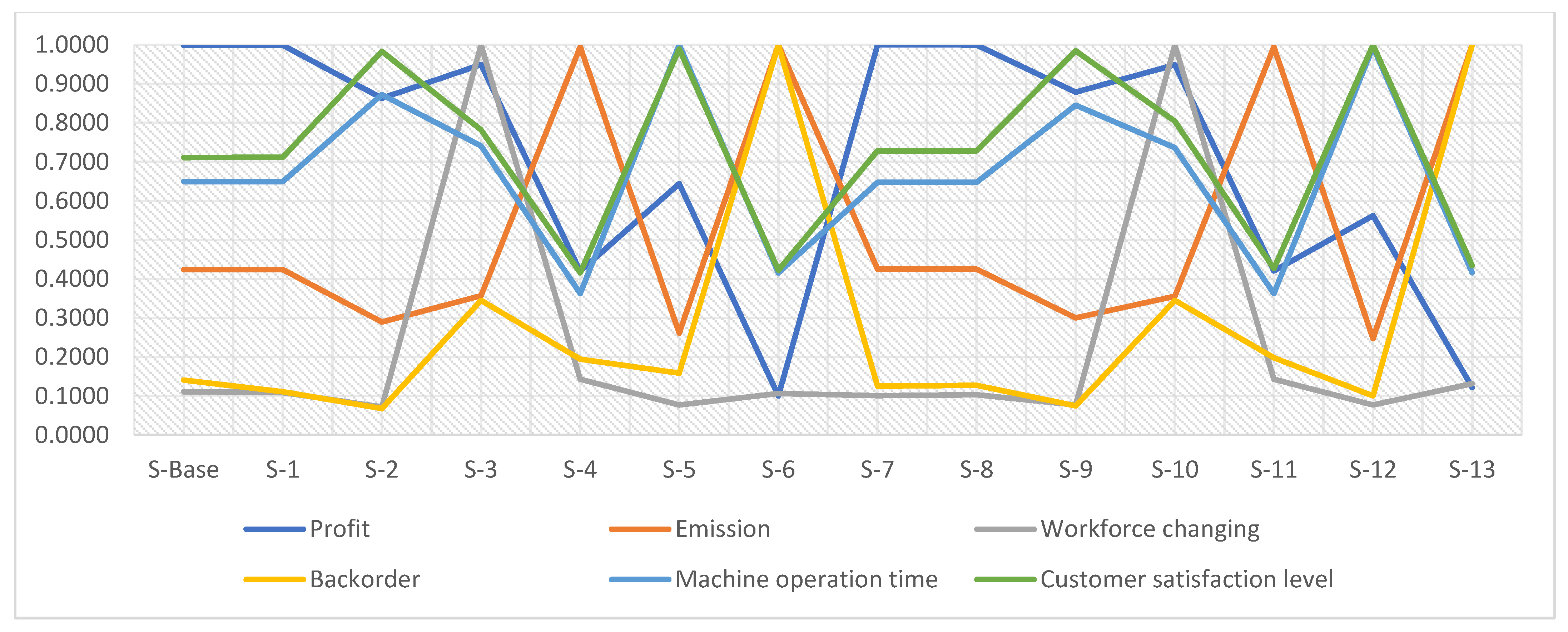
Based on the extreme solutions found above, this study defines the goal values as the first step in applying CGP to the model. Meanwhile, the weighting parameters of the objective functions use the non-negative power of ten to represent the dominant nature or the priority between the objective functions. Table 8 shows that 1% deviation of the goal value of profit is ten times more important than the goal value related to emissions. Similarly, every 1% deviation of the emission-related goal value is more important than a thousand times the goal value relative to machine operation time. In other words, the objective function related to machine operation time is dominated by the emission-related objective function.
As shown in Table 9, the solution obtained from the CGP model has some differences in the value of the objective functions compared to the supplier’s current production plan in 2019 which is named CP solution in this article. According to these results, CGP’s solution resulted in improvements in profitability, emissions, workforce changing and backorder of 21.02%, 37.16%, 30.77% and 23.44% respectively compared to the CP solution. Although the expected value of profit increases, the CGP model also sacrifices the objective functions of machine operation time and customer satisfaction level.
In other words, the CGP solution focuses on effectiveness rather than efficiency. In Figure 3, the production plan of the HB, W, and KB product families is determined by the model to be lower than the CP production plan and uncertain demand. This decision leads to the consequences of low inventory levels as well as reduced production with temporary workers or overtime thereby reducing total costs. Meanwhile, the solution of the model concentrates resources to maintain the production level of more effectiveness product families such as LHB and PB. The CGP model’s production plan of these two product families to chase their uncertain demand.
As one of the factors affecting production levels, the workforce level policy also has the difference between the current operation and the solution of the model as shown in Figure 4. For CP solutions, the workforce is replenished in the first two quarters to ensure production before being maintained in all manufacturing facilities. Meanwhile, the CGP solution shows that the workforce has different changes in manufacturing facilities. The labor force level increased slightly at the VN-1 facility in the first quarter and increased by 50% at the KH facility in the first two quarters. Especially, at the VN-2 facility, the number of full-time workers is downwardly adjusted in the last two quarters of the year to maintain economic effectiveness. In general, the CGP solution suggests a lower workforce level and more variation over time than the manager’s current policy.
According to detailed production plan, shown in Figure 5, CP solution’s regular production plan shows variability in both volume and variety of product families at each manufacturing facility. In other words, each manufacturing facility was in charge of three to four product families with volumes that fluctuate significantly over time. For CGP solution, besides lower total production, the role of production facilities is also more clearly defined to provide stability in production. In which, the product families which involves handbag as LHB and HB are manufactured at facilities in Vietnam. Meanwhile, the remaining production lines are set up at a manufacturing facility in Cambodia. This arrangement helps the production system save time and the cost of re-establishing the production lines.
Figure 6 and Figure 7 shows the CP solution’s production plan by temporary workers and overtime. It can be observed that these two forms of production occur commonly in all manufacturing facilities. In contrast, because of the selection of an effectiveness level of production, CGP profits do not use the temporary workforce in production and only approximately 25,000 units are produced by overtime. This overtime production is equivalent to 11.63% compared to CP solution.
Since production levels are determined more efficiently, the inventory levels of the CGP solution are also lower with the same safety stock policy as shown in Figure 8. In addition, the variety of product families of CP solution also has more disadvantages in warehouse management at manufacturing facilities.
For backorder, both solutions show the backorder that appeared at facility KH where there was the largest planned output as shown in Figure 9. Accordingly, the backorder of the CGP solution is concentrated in the last quarters of the year and is approximately 76.76% equivalent to the CP solution.
To summarize, the solution that the optimization model provides with the CGP multi-objective approach shows advantages in terms of economic efficiency, lower backorder, and environmental and social sustainability factors. On the other hands, this solution sacrifices the utilization of production machines as well as the risk of the absence of goods when market demand increases, because of a low and more secured production level. However, the optimization model in this study still ensures decision-makers’ right to make decisions about satisfaction and sacrifice objectives through weighting parameters.

4.3. Experiments

In this part, the authors examine the changes of the CGP solution according to two factors: Weights of the objective function and probability distributions of demand. For weighting, according to combinatorics, the number of weight combinations increases with a factorial function of the number of objective functions. Thus, there are seven hundred and twenty weight combinations for the six objective functions. However, examining all combinations is ineffective because combinations with similar first, second, and third priority of objective function do not make significant differences in results. Therefore, this study selected seven weighting combinations that have significant differences in priority among the objective functions. For demand’s probability distributions, the expected value of demand is estimated using the three-point estimation method in which PERT distribution and triangular distribution are widely used. The probabilities for the known minimum, most-likely and forecasted maximum demand, which are provide by those distribution, are presented in Table 10.
Accordingly, the authors develop fourteen scenarios based on the two mentioned factors as described and denoted in Table 11. In it, the scenario where its solution has been discussed in the previous section is named S-Base.
Table 12 shows the value of the objective functions for scenarios along with the supplier’s current operations. It can be seen that there are no significant differences in the results between pairs of scenarios with the same weight combinations such as (S-1, S-8), (S-4, S-10), etc. This implies that the difference of the PERT and Triangular distributions does not clearly affect the optimization results. On the other hand, the optimization results of the model clearly show the influence of the weight combinations, which represent the will of the decision-makers on the production system. These scenarios all show their own strengths and weaknesses compared to the rest. However, the solutions of the scenarios S-4, S-6, S-11, and S-13 have low practical application because of low economic efficiency compared to CP solution. The results of scenarios S-5 and S-12 have the same level of customer satisfaction, change in workforce, and machine operation time as CP solution, but greater profits and emissions. The tradeoffs for profit and environmental impact that only creates an improvement in backorder can be difficult to convince production managers. The S-2 and S-9 scenarios are almost identical to the supplier’s current policies, but generate more profits and lower emissions. However, these two scenarios have much higher backorder than the rest. Therefore, when applying them, suppliers need to pay certain attention to the loyalty of customers. Breakthrough scenarios from current operating policy are S-Base, S-1, S-3, S-7, S-8, and S-10 with marked improvement in profitability and sustainable development factors. Among them, the S-3 and S-10 scenarios sacrifice a small profits and environmental impact to achieve less variability in workforce, less backorder, and greater customer satisfaction level.
Finally, the authors normalize the units between the objective functions of the scenarios to scores in the interval [0, 1] in order to analyze the trade-offs between them. The scores presented in Figure 10 show that the S-3 and S-10 scenarios have the greatest number of objective functions whose scores are greater than 0.7. Next is the group of S-Base, S-1, S-7, and S-8 scenarios that have three objective functions with scores between 0.4 and 0.7, besides one objective function that achieves upper extreme scores. The remaining scenarios also have maximum scores at a certain objective function, but the rest are below 0.5.
In conclusion, the optimization model in this study provides managers with solutions that can improve the production planning process. These solutions can be determined under the influence of both subjective and objective factors. Subjective factors represent the will of production managers or decision-makers in choosing the priority between the objective functions. At the same time, market surveys to estimate the objective variability of demand along with its probabilities also increase the model’s effectiveness in practice.

5. Conclusions

In this study, the authors develop a stochastic multi-objective mixed-integer programming model for global sustainable multi-product production planning. The variables of this model assist decision making regarding the quantity of production options including regular production, temporary worker production, overtime production, backorder for each period, and production facilities in many countries. Production resource policies can be adjusted by the managers through model parameters such as facilities’ maximum inventory level, inventory service level, workforce level limitation, overtime limitation, backorder limitation, machine capacity, and so on. The most optimistic, pessimistic, and most-likely values of the demand, along with their PERT probabilities are the basis for the model to calculate the expected value of the demand and the safety stock. The objective functions that the proposed model considers are, respectively, maximizing total profit, minimizing production emissions, minimizing change in workforce, minimizing backorder, maximizing machine operation time, and maximizing customer satisfaction. The multi-objective solution in this study is determined by the Chebyshev variant of the goal programming approach. This variation is able to help goal programming solutions to avoid extreme values of high priority objective functions. Next, scenarios are developed based on the change in the weights of the objective functions and the probability distribution of demand. Analysis of these scenarios helps decision-makers to understand the overall picture of the production system when these two factors fluctuate.
The main contribution of this study was to develop an integrated multiple objectives model as a theoretical reinforcement for the production planning problem. The model considers typical current production system characteristics such as multi-product, multi-facility, multi-period, and uncertainty factors. The proposed model also provides assistance for managers in deciding whether or not the production options are applicable. The options mentioned include regular production, temporary worker production, overtime production, and backorder. The applicability of these production options can be adjusted through the parameters to which the model relates to resource constraints. In addition, the model’s objective functions are defined to ensure both efficient and sustainable development of the production system. Profit maximization, emission minimization, and employment volatility minimization are the objective functions for which the model ensures a balance between the three pillars of sustainable development: Economic, environmental, and social. At the same time, the objective functions that minimize backorder, maximize machine uptime, and maximize customer satisfaction towards optimizing production system efficiency. In order to achieve solutions that are weighted and balanced at the same time for these objective functions, this study proposes the Chebyshev goal programming approach. Another contribution of this study is the development and evaluation of scenarios that depend on the random distributions of uncertain demand and the weights of the objective functions from the point of view of the production managers. This assessment is a useful reference for managers to adjust their production plans for uncertainties and production changes according to the global situation.
Future studies may consider the complexity of other random distributions in terms of the uncertainties of demand as well as production resources. In addition, the advantages of machine learning are also suitable approaches to predict the effectiveness of scenarios as their number may increase exponentially.

Author Contributions

Conceptualization, N.-L.N.; methodology, C.-N.W., N.-L.N.; formal analysis, N.-L.N., and T.T.T.T.; investigation, N.-L.N.; data curation, N.-L.N.; writing—original draft preparation, N.-L.N., and T.T.T.T.; writing—review and editing, C.-N.W., N.-L.N.; project administration, C.-N.W.; funding acquisition, C.-N.W. All authors have read and agreed to the published version of the manuscript.

Funding

The research was partly supported by the National Kaohsiung University of Science and Technology, and MOST 109-2622-E-992-026 from the Ministry of Sciences and Technology in Taiwan.

Acknowledgments

The authors appreciate the support from the National Kaohsiung University of Science and Technology and the Ministry of Sciences and Technology in Taiwan.

Conflicts of Interest

The authors declare no conflict of interest.

Appendix A

Table A1. Production planning linear programming models.
AuthorYearProblem CharacteristicsMultiple ObjectivesProduction Options
Uncertainty FactorMultiple FacilityMultiple ProductEconomyEnvironmentOthersPart-Time Worker ProductionBackorderOvertime
Bakir, M.A. et al.1998X X
Vasant, P. et al.2004X X
Kanyalkar, A.P. et al.2005 XXX
Vasant, P.M.2006X X
Li, C. et al.2008X XX
Orcun, S. et al.2009X X
Kezemi Zanjani, M. et al.2009X XX X
Elamvazuthi, I. et al.2009X XX
Leung, S.C.H. and Chan, S.S.W.2009 XXX X XX
Ozsan, O. et al.2010 XX
Baykasoglu, A. and Goken, T.2010X XX XX
Leung, S.C.H. et al.2010 XXX XXXX
Gramani, M.C.N. et al.2011 XX
Sillekens, T. et al.2011 XX
Zhang, X. et al.2011X XX X
Ning, Y. et al.2012X XX XX
Kezemi Zanjani, M. et al.2013X XX X
Mortezaei, N. et al.2013XXXX
Munhoz, J.R. et al.2014 XX
Madadi, N. and Wong, K.Y.2014X XX XX
Davizón, Y. et al.2015 X
Kalaf, B.A. et al.2015X XX X
Modarres, M. and Izadpanahi, E.2016X XXX X
Campo, E.A. et al.2018 X
Komsiyah, S. et al.2018X XX
Hahn, G.J. and Brandenburg, M.2018 XXX XX
Tsai, W.-H.2018 XXX X
Djordjevic, I. et al.2019X X
Tirkolaee, E.B. et al.2019X X X XX
Proposed modelXXXXXXXXX

References

  1. Sustainable Production Methods in Textile Industry. 2019. Available online: https://www.intechopen.com/books/textile-industry-and-environment/sustainable-production-methods-in-textile-industry (accessed on 20 December 2020).
  2. Huynh, N.-T.; Chien, C.-F. A hybrid multi-subpopulation genetic algorithm for textile batch dyeing scheduling and an empirical study. Comput. Ind. Eng. 2018, 125, 615–627. [Google Scholar] [CrossRef]
  3. Campo, E.A.; Cano, J.A.C.; Gómez-Montoya, R.A. Linear Programming for Aggregate Production Planning in a Textile Company. Fibres Text. East. Eur. 2018, 26, 13–19. [Google Scholar] [CrossRef]
  4. Pochet, Y. Mathematical Programming Models and Formulations for Deterministic Production Planning Problems. In Computational Combinatorial Optimization; Springer: Berlin/Heidelberg, Germany, 2001; pp. 57–111. [Google Scholar]
  5. Salomon, M. Deterministic Lotsizing Models for Production Planning; Springer-Verlag: Berlin/Heidelberg, Germany, 1991. [Google Scholar]
  6. Du, J.; Liang, L.; Chen, Y.; Bi, G.-B. DEA-based production planning. Omega-Int. J. Manag. S. 2010, 38, 105–112. [Google Scholar] [CrossRef]
  7. Charne, A.; Cooper, W.W.; Rhodes, E. Measuring the efficiency of decision making units. Eur. J. Oper. Res. 1978, 2, 429–444. [Google Scholar] [CrossRef]
  8. Wang, C.-N.; Dang, T.-T.; Nguyen, N.-A.-T. A Computational Model for Determining Levels of Factors in Inventory Management Using Response Surface Methodology. Mathematics 2020, 8, 1210. [Google Scholar] [CrossRef]
  9. Bagshaw, K.B. A Review of Quantitative Analysis (QA) in Production Planning Decisions Using the Linear Programming Model. Am. J. Oper. Res. 2019, 9, 255–269. [Google Scholar] [CrossRef] [Green Version]
  10. Kanyalkar, A.P.; Adil, G.K. An integrated aggregate and detailed planning in a multi-site production environment using linear programming. Int. J. Prod. Res. 2005, 43, 4431–4454. [Google Scholar] [CrossRef]
  11. Davizón, Y.; Martínez-Olvera, C.; Soto, R.; Hinojosa, C.; Espino-Román, P. Optimal Control Approaches to the Aggregate Production Planning Problem. Sustainability 2015, 7, 16324–16339. [Google Scholar] [CrossRef] [Green Version]
  12. Ozsan, O.; Simsir, F.; Pamukcu, C. Application of Linear Programming in Production Planning at Marble Processing Plants. J. Min. Sci. 2010, 46, 57–65. [Google Scholar] [CrossRef]
  13. Gramani, M.C.N.; França, P.M.; Arenales, M.N. A linear optimization approach to the combined production planning model. J. Frankl. Inst. 2011, 348, 1523–1536. [Google Scholar] [CrossRef]
  14. Sillekens, T.; Koberstein, A.; Suhl, L. Aggregate production planning in the automotive industry with special consideration of workforce flexibility. Int. J. Prod. Res. 2011, 49, 5055–5078. [Google Scholar] [CrossRef] [Green Version]
  15. Munhoz, J.R.; Morabito, R. Optimization approaches to support decision making in the production planning of a citrus company: A Brazilian case study. Comput. Electron. Agric. 2014, 107, 45–57. [Google Scholar] [CrossRef]
  16. Cheraghalikhani, A.; Khoshalhan, F.; Mokhtari, H. Aggregate production planning: A literature review and future research directions. Int. J. Ind. Eng. Comput. 2019, 309–330. [Google Scholar] [CrossRef]
  17. Mula, J.; Poler, R.; García-Sabater, J.P.; Lario, F.C. Models for production planning under uncertainty: A review. Int. J. Prod. Econ. 2006, 103, 271–285. [Google Scholar] [CrossRef] [Green Version]
  18. Bakir, M.A.; Byrne, M.D. Stochastic linear optimisation of an MPMP production planning model. Int. J. Prod. Econ. 1998, 55, 87–96. [Google Scholar] [CrossRef]
  19. Vasant, P.; Nagarajan, R.; Yaacob, S. Decision making in industrial production planning using fuzzy linear programming. IMA J. Manag. Math. 2004, 15, 53–65. [Google Scholar] [CrossRef]
  20. Elamvazuthi, I.; Ganesan, T.; Vasant, P.; Webb, J.F. Application of a Fuzzy Programming Technique to Production Planning in the Textile Industry. Int. J. Comput. Sci. Inf. Secur. 2009, 6, 238–243. [Google Scholar]
  21. Madadi, N.; Wong, K.Y. A Multiobjective Fuzzy Aggregate Production Planning Model Considering Real Capacity and Quality of Products. Math. Probl. Eng. 2014, 2014, 1–15. [Google Scholar] [CrossRef]
  22. Vasant, P.M. Fuzzy production planning and its application to decision making. J. Intell. Manuf. 2006, 17, 5–12. [Google Scholar] [CrossRef]
  23. Djordjevic, I.; Petrovic, D.; Stojic, G. A fuzzy linear programming model for aggregated production planning (APP) in the automotive industry. Comput. Ind. 2019, 110, 48–63. [Google Scholar] [CrossRef]
  24. Kalaf, B.A.; Bakar, R.A.; Soon, L.L.; Monsi, M.B.; Bakheet, A.J.K.; Abbas, I.T. A Modified Fuzzy Multi-Objective Linear Programming to Solve Aggregate Production Planning. Int. J. Pure Appl. Math. 2015, 104, 339–352. [Google Scholar] [CrossRef] [Green Version]
  25. Baykasoglu, A.; Gocken, T. Multi-objective aggregate production planning with fuzzy parameters. Adv. Eng. Softw. 2010, 41, 1124–1131. [Google Scholar] [CrossRef]
  26. Mortezaei, N.; Zulkifli, N.; Hong, T.S.; Yusuff, R.M. Multi-objective aggregate production planning model with fuzzy parameters and its solving methods. Life Sci. J. 2013, 10, 2406–2414. [Google Scholar]
  27. Ning, Y.; Liu, J.; Yan, L. Uncertain aggregate production planning. Soft Comput. 2012, 17, 617–624. [Google Scholar] [CrossRef]
  28. Orcun, S.; Uzsoy, R.; Kempf, K.G. An integrated production planning model with load-dependent lead-times and safety stocks. Comput. Chem. Eng. 2009, 33, 2159–2163. [Google Scholar] [CrossRef]
  29. Li, C.; He, X.; Chen, B.; Xu, Q.; Liu, C. A Hybrid Programming Model for Optimal Production Planning under Demand Uncertainty in Refinery. Chin. J. Chem. Eng. 2008, 16, 241–246. [Google Scholar] [CrossRef]
  30. Kazemi Zanjani, M.; Nourelfath, M.; Ait-Kadi, D. A multi-stage stochastic programming approach for production planning with uncertainty in the quality of raw materials and demand. Int. J. Prod. Res. 2009, 48, 4701–4723. [Google Scholar] [CrossRef]
  31. Zhang, X.; Prajapati, M.; Peden, E. A stochastic production planning model under uncertain seasonal demand and market growth. Int. J. Prod. Res. 2011, 49, 1957–1975. [Google Scholar] [CrossRef]
  32. Kazemi Zanjani, M.; Ait-Kadi, D.; Nourelfath, M. A stochastic programming approach for sawmill production planning. Int. J. Math. Oper. Res. 2013, 5, 1–18. [Google Scholar] [CrossRef]
  33. Komsiyah, S.; Meiliana; Centika, H.E. A Fuzzy Goal Programming Model for Production Planning in Furniture Company. Procedia Comput. Sci. 2018, 135, 544–552. [Google Scholar] [CrossRef]
  34. Tirkolaee, E.B.; Goli, A.; Weber, G.-W. Multi-objective Aggregate Production Planning Model Considering Overtime and Outsourcing Options Under Fuzzy Seasonal Demand. In Advances in Manufacturing II; Springer International Publishing: Cham, Switzerland, 2019. [Google Scholar]
  35. Leung, S.C.H.; Chan, S.S.W. A goal programming model for aggregate production planning with resource utilization constraint. Comput. Ind. Eng. 2009, 56, 1053–1064. [Google Scholar] [CrossRef]
  36. Leung, S.C.H.; Wu, Y.; Lai, K.K. Multi-site aggregate production planning with multiple objectives: A goal programming approach. Prod. Plan. Control 2010, 14, 425–436. [Google Scholar] [CrossRef]
  37. Hahn, G.J.; Brandenburg, M. A sustainable aggregate production planning model for the chemical process industry. Comput. Oper. Res. 2018, 94, 154–168. [Google Scholar] [CrossRef]
  38. Tsai, W.-H. Green Production Planning and Control for the Textile Industry by Using Mathematical Programming and Industry 4.0 Techniques. Energies 2018, 11, 2072. [Google Scholar] [CrossRef] [Green Version]
  39. Modarres, M.; Izadpanahi, E. Aggregate production planning by focusing on energy saving: A robust optimization approach. J. Clean. Prod. 2016, 133, 1074–1085. [Google Scholar] [CrossRef]
  40. Dasović, B.; Galić, M.; Klanšek, U. A Survey on Integration of Optimization and Project Management Tools for Sustainable Construction Scheduling. Sustainability 2020, 12, 3405. [Google Scholar] [CrossRef] [Green Version]
  41. Valenko, T.; Klanšek, U. An integration of spreadsheet and project management software for cost optimal time scheduling in construction. Organ. Technol. Manag. Constr. Int. J. 2017, 9, 1627–1637. [Google Scholar] [CrossRef] [Green Version]
  42. Nahmias, S.; Olsen, T.L. Production and Operations Analysis, 7th ed.; Waveland Press, Inc.: Grove, IL, USA, 2015. [Google Scholar]
  43. Çay, A. Energy consumption and energy saving potential in clothing industry. Energy 2018, 159, 74–85. [Google Scholar] [CrossRef]
  44. List of Grid Emission Factors. 2020. Available online: https://pub.iges.or.jp/pub/iges-list-grid-emission-factors (accessed on 21 January 2021).
Figure 1. Total production in 2019 (unit).
Mathematics 09 00483 g001
Figure 2. Required processing time (hour/unit). (a) Operator (b) Machine.
Mathematics 09 00483 g002
Figure 3. Expected sale and expected demand (unit).
Mathematics 09 00483 g003
Figure 4. Workforce level changing (man). (a) CP (b) CGP.
Mathematics 09 00483 g004
Figure 5. Regular production plan (unit). (a) CP (b) CGP.
Mathematics 09 00483 g005
Figure 6. CP solution’s temporary worker production plan (unit).
Mathematics 09 00483 g006
Figure 7. CP solution’s overtime production (unit).
Mathematics 09 00483 g007
Figure 8. Inventory level (unit). (a) CP (b) CGP.
Mathematics 09 00483 g008
Figure 9. Backorder level in KH facility (unit).
Mathematics 09 00483 g009
Figure 10. Scenario’s normalized score.
Mathematics 09 00483 g010
Table 1. Production planning model classification.
Single ObjectiveMultiple Objective
Deterministic modelsGroup 1Group 2
Uncertainty modelsFuzzy modelsGroup 3Group 4
Stochastic modelsGroup 5Group 6
Table 2. Sets.
Table 2. Sets.
SetIndicesDescription
IiThe set of the product families
JjThe set of the factories
TtThe set of the planning periods
KKThe set of objective functions
Table 3. Parameters.
GroupParameterDescriptionUnit
1 P i The unit sell price of product iK VND/unit
P C i j F The unit production cost by full-time workersK VND/unit
P C i j T The unit production cost by temporary workers K VND/unit
O T C i j The unit production cost by full-time workers at overtimeK VND/unit
L C j F The labor cost of fulltime worker K VND/man-period
L C j T The labor cost of temporary worker K VND/man-period
L C j O T The labor cost of fulltime worker at overtimeK VND/man-period
I C i j The unit inventory cost to hold a product at the end of each periodK VND/unit
B O C i j The unit backorder cost for a product at the end of each periodK VND/unit
H C j The hiring cost for one full-time workerK VND/man
F C j The firing cost for one full-time workerK VND/man
2 I L j t Maximum inventory capacity in factory j at period tUnits
B O L i t Maximum backorder in of product i at period tUnits
W j m i n Minimum workforce level of full-time worker available in factory j in each periodMan
W j m a x Maximum work-force level of full-time worker available in factory j in each periodMan
T P L j t The temporary worker time limit in factory j at period tHour
M L j t The machine time capacity in factory j at period tMachine-hour
3 D i t m i n Minimum known demand of product i at period tUnits
D i t m o s t Most-likely demand of product i at period tUnits
D i t m a x Maximum forecasted demand of product i at period tUnits
σ i m i n Standard deviation of minimum known demand standard deviation of product i Units
σ i m o s t Standard deviation of most-likely demand of product iUnits
σ i m a x Standard deviation of maximum forecasted demand of product iUnits
P r m a x The probability of forecasted maximum demand%
P r m o s t The probability of most-likely demand%
P r m i n The probability of minimum known demand%
4 P T i F The processing time for product i by full-time workersHour/unit
P T i T The processing time for product i by temporary workersHour/unit
M T i F The machine time for product i operated by full-time workersMachine-hour/unit
M T i T The machine time for product i operated by temporary workersMachine-hour/unit
5 δ j The working hour of full-time workers in factory j in each periodHour/man-period
W L C j The fraction of workforce allowable for variation in each period%
α j The fraction of overtime hours in factory j used in each period%
B Z i The production batch size of product iUnits/batch
E F j CO2 Emission factor of factory jtCO2/mwh
SE Specific electricity use for productionmwh/unit
zThe inverse distribution function of a standard normal distribution with cumulative probability
βThe proportion of demand met from stock (service level Type II)%
G k The aspiration level of objective function k
W E k The weight of objective function k
Table 4. Decision variables.
Decision VariableTypeDescriptionUnit
S i t IntegerThe quantity of product i sold at period tUnits
x i j t IntegerThe quantity of product i manufactured from factory j by full-time worker at regular time at period tBatch
y i j t IntegerThe quantity of product i manufactured from factory j by temporary worker in regular time at period tBatch
v i j t IntegerThe quantity of product i manufactured from factory j by full-time worker in overtime at period tBatch
W j t IntegerThe number of fulltime workers required in factory j at period tMan
H j t IntegerThe number of fulltime workers hired in factory j at period tMan
F j t IntegerThe number of fulltime workers laid-off in factory j at period tMan
O T j t FloatThe overtime of fulltime workers in factory j at period tHour
T P T j t FloatThe labor time of temporary workers in factory j at period tHour
M P T j t FloatThe machine using time in factory j at period tHour
I i j t IntegerThe inventory of product i in factory j at the end of period tBatch
B i j t IntegerThe backorder of product i in factory j at the end of period tBatch
θ j t Binary = { 1 i f   f a c t o r y   j   h i r i n g   w o r k e r   a t   p e r i o d   t 0 o t h e r w i s e
φ i j t Binary = { 1 i f   p r o d u c t   i   p r o d u c e d   f r o m   f a c t o r y   j   a t   p e r i o d   t 0 o t h e r w i s e
o k Integer/floatThe deviation variable of overachievement of the goal G k
u k floatThe deviation variable of underachievement of the goal G k
ωFloatThe maximal deviation from amongst the goals
Table 5. Facility production policy.
FacilityVN-1VN-2KH
Workforce change rate (%)20%20%30%
Initial workforce (man)15070100
Minimum workforce level (man)15050100
Maximum workforce (man)200100150
Overtime limit (%)20%20%40%
Maximum inventory level (unit/period)20,00015,00020,000
Machine capacity (hour)62,40049,92062,400
Table 6. Optimization problem size.
ConstraintsDecision VariablesNon-Zero Coefficients
BinaryIntegerFloat
88072358475225
Table 7. Objective function payoff matrix.
Objective Function ValueMaximize ProfitMinimize EmissionMinimize Workforce ChangingMinimize BackorderMaximize Machine Operation TimeMaximize Customer Satisfaction Level
Profit (mil. VND)516,838 88,107 138,952 48,253 245,826 391,505
Emission (tCO2)65.06 19.59 43.17 49.38 89.5483.44
Workforce changing (man)132940198130130
Backorder (Unit)11,550 14,000 7000 010,900 11,950
Machine operation time (hour)473,753 230,519 277,133 294,848 609,647 572,256
Customer satisfaction level (%)74.4536.4044.1445.2885.9788.42
CPU time (second)2.972.512.372.364.1028.89
No. of Iterations13,203267912311334,6502,187,084
Table 8. Objective function’s goal value and weight.
Objective FunctionGoal Value (Gk)Weight (WEk)
Maximize profit516,838105
Minimize emission19.59104
Minimize workforce changing0103
Minimize backorder0102
Maximize machine operation time609,647101
Maximize customer satisfaction level88.42100
Table 9. Chebyshev goal programming solution’s objective function value.
Objective Function ValueCPCGPImprovement
Profit (mil. VND)363,093439,41721.02%
Emission (tCO2)77.8648.9337.16%
Workforce changing (man)1309030.77%
Backorder (Unit)9250710023.24%
Machine operation time (hour)591,511394,361−33.33%
Customer satisfaction level (%)86.84%62.26%−28.30%
Table 10. Demand probability distributions.
DistributionMinimum Demand Probability
Prmin
Most-Likely Demand Probability
Prmost
Maximum Demand Probability
Prmax
Program evaluation and review technique (PERT) distribution1/64/61/6
Triangular distribution1/31/31/3
Table 11. Experiment scenarios.
ScenarioDemand Probability DistributionObjective Function Weight
Maximize ProfitMinimize EmissionMinimize Workforce ChangingMinimize BackorderMaximize Machine Operation TimeMaximize Customer Satisfaction Level
S-BasePERT100,00010,0001000100101
S-1100,00010,0001101001000
S-210,0001000110100100,000
S-310,000100100,0001000110
S-410,000100,0001011001000
S-51000100101100,00010,000
S-610010,00010100,00010001
S-7Triangular 100,00010,0001000100101
S-8100,00010,0001101001000
S-910,0001000110100100,000
S-1010,000100100,0001000110
S-1110,000100,0001011001000
S-121000100101100,00010,000
S-1310010,00010100,00010001
Table 12. Scenario objective function value.
ScenarioProfit
(mil. VND)
Emission
(tCO2)
Workforce Changing
(man)
Backorder
(Unit)
Machine Operation Time
(hour)
Customer Satisfaction Level
(%)
CP363,09377.85801309250591,51186.84%
S-Base439,41748.9308907100394,36162.26%
S-1439,42448.9305929000394,23662.32%
S-2379,72271.560313914,750529,42586.08%
S-3417,55358.0736102900449,70068.46%
S-4184,56220.8473705150220,10836.40%
S-5283,31779.38441306300606,89486.60%
S-644,17720.7368941000252,36636.98%
S-7439,88948.7600998000392,80963.77%
S-8439,88048.7576977850392,88363.78%
S-9386,57569.131813013,400513,12786.18%
S-10417,35058.2894102900446,74770.40%
S-11185,07020.8426705050219,94137.34%
S-12247,33383.98291309950603,76687.53%
S-1353,64820.7344761000252,52238.03%
Publisher’s Note: MDPI stays neutral with regard to jurisdictional claims in published maps and institutional affiliations.

