Stochastic Modeling of Plant Virus Propagation with Biological Control

Abstract

Plants are vital for man and many species. They are sources of food, medicine, fiber for clothes and materials for shelter. They are a fundamental part of a healthy environment. However, plants are subject to virus diseases. In plants most of the virus propagation is done by a vector. The traditional way of controlling the insects is to use insecticides that have a negative effect on the environment. A more environmentally friendly way to control the insects is to use predators that will prey on the vector, such as birds or bats. In this paper we modify a plant-virus propagation model with delays. The model is written using delay differential equations. However, it can also be expressed in terms of biochemical reactions, which is more realistic for small populations. Since there are always variations in the populations, errors in the measured values and uncertainties, we use two methods to introduce randomness: stochastic differential equations and the Gillespie algorithm. We present numerical simulations. The Gillespie method produces good results for plant-virus population models.

1. Introduction

Viruses cause a great number of diseases in plants. In [1] the authors gave a review of the top ten viruses. In plants the most common way that viruses are propagated is by means of a vector, usually insects. A carrier insect will bite an infected plant, thereby infecting it [2]. Mathematical models of virus-caused diseases in plants can be used to better understand the processes involved [3,4,5,6,7]. Viruses take time to propagate and replicate. These effects can be taken into account by considering latent populations [8,9]. In this paper we present three different mathematical models of virus propagation in plants with a predator used as a biological control of the insects that transmit the virus [10]. The description of the model is given in terms of differential equations and also biochemical style reactions. Models based on differential equations are built on the assumption that the number of individuals is very large, which is not always the case. The model that we use incorporating delays in the spread of the virus in both plants and vectors is based on [11]. An extension to optimal control through the use of predators and insecticide is in [12]. The authors in [13] introduced a delay to the model in [8] to account for the incubation period of the plants. In [14] there is a different model with delays. Populations have variabilities and there are errors in measuring and estimating the parameters involved. The variations and uncertainties in the populations and environmental conditions can be modeled by introducing randomness or stochasticity into the models. One common way is to use stochastic differential equations [15,16]. A second way is to consider that some of the coefficients in the model are random variables, as in the method of polynomial chaos [17,18]. Another method is to consider discrete populations and work with Markov chains [19,20,21], including working with the master equation [22]. Models based on continuous time Markov chains usually use the stochastic simulation algorithm of Gillespie [23,24]. Very complex models of plant viral assembly have been presented in [25,26]. Mathematical models of populations involve a series of simplifying hypotheses [27]. One of them is that the individuals in each population group have the same properties. Another usual one is that the populations are homogeneously distributed. A third one is that the number of individuals is large. Based on these simplifications, the populations can be assumed to be continuous and the model can be described in terms of differential equations or maybe delay differential equations. An alternative method of developing mathematical population models is to consider the interactions between individuals to be a reaction. For example, an individual of the class susceptible S dying can be described by the following reaction: $S\stackrel{k}{\to }$. Here the blank space denotes an empty population. Using differential equations, it would be $\frac{dS}{dt}=-kS.$ Additionally, the interaction between a susceptible S and an infective I leading to a new infective is $S+I\stackrel{\beta /N}{\to }I+I$, while the corresponding differential equation is $\frac{dS}{dt}=-\beta SI/N$. k is the death rate, $\beta /N$ is the infection rate divided by the total population N in the differential equations and both are the reaction rates in the corresponding reactions. This is the formulation preferred by biology and chemistry researchers. By dividing the time period of interest into subintervals and considering that all the different reactions happen at the same instant in each subinterval, the reaction system can be converted into a system of discrete equations giving the change of each population in the time subinterval. By letting the length of the time subintervals go to zero, a system of differential equations is obtained. However, if the number of individuals is not very large, as is the case in our plant-virus propagation problem or in cell processes in systems biology, the limiting process introduces errors, and the assumption that all reactions occur simultaneously is not a good one. An alternative is to consider the reactions as continuous time Markov chains [28]. This assumption leads to the stochastic simulation algorithm, or Gillespie algorithm [23,24], and its variations.

We apply this method to a simple susceptibles (S), infectives (I) and recovereds (R) (SIR) epidemic model and to a predator–prey model. The objective of presenting these two simple models is to introduce the basic ideas of writing ordinary differential equations as biochemical reactions. Then we apply them to our main interest, which is a model of virus propagation consisting of six populations, susceptible plants, infective plants, recovered plants, susceptible insects, infective insects and predators. For this virus propagation model, we consider three cases: all the interactions are mass actions—some of them are saturated and some are saturated with delays. The saturated interactions are modeled using Holling type 2 functionals [29]. We also write the models as a system of reactions. Simulations were performed using the stochastic simulation algorithm. For comparison purposes, the corresponding system of differential equations is solve numerically, and finally white noise is added to the differential equation systems to obtain stochastic differential equations and simulate them numerically. The rest of the paper is organized as follows. In Section 2, the development of the models is presented, as is the addition of stochasticity to the models to take into account the variability in the populations and other uncertainties always present in the processes modeled. Next, the virus propagation models and the numerical methods are described. Section 3 shows sample numerical simulations. In Section 4, the results are discussed. Finally there is a conclusions section.

2. Materials and Methods

2.1. Mathematical Modeling

Mathematical models for populations are usually given in terms of differential equations or difference equations. The differential equations may be ordinary, delay, partial or even fractional. However, the models may also be given by describing the interactions between the different population groups and the rate at which they happen. That is, they may be described in terms of reactions with the same structure as biochemical reactions. Therefore, we can write differential equations arising from mathematical biology as reactions. For example $\frac{dS}{dt}=-kS$ can be written as $S\stackrel{kS}{\to }$, where the ban space means that the population disappears. As a second example, $\frac{dS}{dt}=-\beta SI$ is equivalent to $S+I\stackrel{\beta SI}{\to }I+I$. Sometimes the quantity written on top of the arrow is the number of times the reaction occurs in a population (propensity), and sometimes only the reaction rate constant is included. We use the propensities.

As an illustration on the basic ideas of converting differential equations into biochemical reactions, consider the well known SIR model giving the interaction of susceptibles (S), infectives (I) and recovereds (R) [27]:

$$\begin{array}{cc}\hfill \frac{dS}{dt}& =-\frac{\beta SI}{N}\hfill \\ \hfill \frac{dI}{dt}& =\frac{\beta SI}{N}-\gamma I\hfill \\ \hfill \frac{dR}{dt}& =\gamma I.\hfill \end{array}$$

(1)

In writing the model as a system of reactions, we obtain a reaction for each distinct term on the right hand-side of the differential equations. In this example we have two such terms, $\frac{\beta SI}{N}$ and $\gamma I$. The first term has the reaction of S and I. The second gives the change of I to another population. If the differential equation that has the derivative of a population includes the given term on the right-hand side with a positive sign, then the product of the reaction is that population. Hence, by writing the model as reactions between the populations we have

$$\begin{array}{cc}\hfill I+S& \stackrel{SI\beta /N}{\to }2I\hfill \\ \hfill I& \stackrel{\gamma I}{\to }R.\hfill \end{array}$$

(2)

The first reaction is the conversion of one S into one I, and the second one is the conversion of one I into one R.

The system of reactions is not unique. This non-uniqueness has been established by [30]. In this case a more complex system is

$$\begin{array}{cc}\hfill I+S& \stackrel{SI\beta /N}{\to }I\hfill \\ \hfill I+S& \stackrel{SI\beta /N}{\to }S+2I\hfill \\ \hfill I& \stackrel{\gamma I}{\to }R.\hfill \end{array}$$

(3)

In this second set of reactions, S loses one member first and in the next reaction I gains one. The reaction happens in two steps. We use the simpler formulation with S converting directly into I. However, below we will show that both formulations give the same system of differential equations.

To convert the model given in terms of reactions to a differential equation model, consider a time interval $[t,t+\delta t]$ and assume that all the reactions occur at the same instant in this interval. For the reaction system (3) we have

$$\begin{array}{cc}\hfill I(t+\delta t)& =I\left(t\right)+\delta t\left(S\right(t\left)I\right(t\left)\right)\beta /N\hfill \\ \hfill S(t+\delta t)+2I(t+\delta t)& =S\left(t\right)+2I\left(t\right)+\delta t\left(S\right(t\left)I\right(t\left)\right)\beta /N\hfill \\ \hfill R(t+\delta t)& =R\left(t\right)+I\left(t\right)\gamma .\hfill \end{array}$$

Assuming that the three populations are large enough, so that all the reactions happen even for very small $\delta t$, we can take the limit as $t\to 0$ to get

$$\begin{array}{cc}\hfill \frac{dI}{dt}& =\left(IS\right)\beta /N\hfill \\ \hfill \frac{d(S+2I)}{dt}& =\left(IS\right)\beta /N\hfill \\ \hfill \frac{dR}{dt}& =\gamma I.\hfill \end{array}$$

By subtracting the first equation from the second, we obtain the original system of differential Equation (1). Similarly, using the reactions in (2), we obtain (1) directly. In [31], the authors used biochemical reactions to model SIR processes. Reference [32] also included implementations of the Gillespie algorithm for the SIR model.

As a second example, consider a simple predator–prey model as given by Lotka and Volterra [27]:

$$\begin{array}{cc}\hfill \frac{dx}{dt}& =(b-py)x\hfill \\ \hfill \frac{dy}{dt}& =(rx-d)y,\hfill \end{array}$$

(4)

where x is the prey and y is the predator. The corresponding system of reactions is

$$\begin{array}{cc}\hfill x& \stackrel{bx}{\to }2x\hfill \\ \hfill x+y& \stackrel{pxy}{\to }y\hfill \\ \hfill x+y& \stackrel{rxy}{\to }x+2y\hfill \\ \hfill y& \stackrel{dy}{\to }\hfill \end{array}$$

(5)

The first reaction is the birth of new prey, the second reaction is the elimination of prey by predators, the third one is the conversion of dead prey into new predators and the last one is the death of predators. The conversion of prey into predators needs to be in two reactions, since one killed prey does not convert into one new predator.

Even though it is straightforward to convert a population model based on differential equations to one described by reactions, there exist software packages that will automate the process. Biocham [33] http://lifeware.inria.fr/biocham4/ (accessed on 12 December 2020) will convert systems of ordinary differential equations with general interactions between populations written in xppauto format [34] to biochemical reactions. Moccasin [35] uses biocham and adds an interface for the MATLAB format of differential equations. Both programs write the equations in SBML [36], a widely used machine-readable description of biochemical reactions.

2.2. Stochastic Modeling

In order to produce more realistic results, mathematical models need to take into account the existence of errors in the observed or measured population data; variability in the populations; and uncertainties such as missing data and lack of knowledge.

These uncertainties can be modeled using random differential equations wherein it is considered that the parameters are random variables [37]. Another method is to use discrete or continuous time Markov chain models [38,39]. A different method consists of introducing the uncertainties as white noise and obtaining stochastic differential equations [16,40]. In this paper we only consider the second and third methods.

2.2.1. Continuous Time Markov Chain Models

As mentioned above, population models can be described in terms of biochemical-type reactions. A Markov chain is a stochastic process in which the probability of an event happening depends on a sequence of possible events, in which the probability of each event depends only on the previous event [28,39]. In a discrete time Markov chain, the changes of state happen at fixed points in time. In a continuous time Markov chain, the changes of state can happen at any time. Each reaction is a random event that has a given probability of happening. This probability is a function of the reaction rate and of the numbers of individuals of the populations involved. Since the reactions can occur at any time, the reactions are continuous time Markov chains. The master chemical equation for a reaction is the time evolution equation for the probability distribution over the state space of a Markov process. This is derived by substituting the transitional probability of the Markov process into the Chapman–Kolmogorov equation [41,42]. For a system of reactions, the master chemical equation is a system of ordinary differential equations that is hard to solve either analytically or numerically [43,44]. An alternative is the stochastic simulation algorithm (SSA) proposed by Gillespie [23] which produces numerical realizations. The next reaction and the time until it occurs are determined by Monte Carlo simulations involving the propensities of the reactions, and the process is repeated. The processes are Poisson processes with exponentially distributed transition times. Improvements on Gillespie’s direct method are given in [24,45]. The SSA works with populations which should not be very small. Numerical implementations are, for example, in [46,47,48].

2.2.2. Stochastic Differential Equations

Randomness can be added to an ordinary differential equation $dx=f(x,t)dt,x\left(t_0\right)=x_0$ by including a white noise process [16,40]. A stochastic differential equation is given by

$$dX(t,\omega )=f\left(X\right(t,\omega ),t)+g\left(X\right(t,\omega ),t)dW(t,\omega ),$$

where $\omega$ is an element of the sample space and $X=X(t,\omega )$ is a stochastic process. The initial condition $X(0,\omega )=X_0$ is taken to be known with probability one. A Brownian motion or Wiener process is formed by a sequence of random variables parameterized by time that are independent and identically distributed (iid). A stochastic process $W\left(t\right),t\in [0,\infty ]$ is a Wiener process (or a standard Brownian motion) if it satisfies: (i) It is defined for $t\ge 0$ with $W_0=0$; (ii) if $0\le s<t<\infty$, then $W\left(t\right)-W\left(s\right)$ is normally distributed with mean 0 and variance $t-s$, that is, $W\left(t\right)-W\left(s\right)\sim N(0,t-s)$; (iii) if $0\le r<s<t<\infty$, the increments $W\left(t\right)-W\left(s\right)$ and $W\left(s\right)-W\left(r\right)$ are independent.

The noise term is called additive if it is independent of the population. This noise is also called environmental noise. If the noise term is proportional to the population, it is called multiplicative. These two are the most common types of white noise used, but they can have more complicated forms [49,50,51,52]. For uniform populations the environmental noise may be dominant. However, populations usually have variations. Demographic stochasticity is usually defined as the variation in the time evolution of a small population due to the randomness of individual birth, death, infection and other rates. However, the term can also be used for populations of any size. It can be related to stochasticity with multiplicative white noise by considering that the rates have a deterministic part plus a stochastic one. Additionally, environmental fluctuations may be related to overpopulation in ways such as shortage of food, increased aggression toward each other, etc. Therefore, a reasonable way to modify the deterministic equation is to consider introducing randomness that is proportional to the size of the population. However, this is just an assumption that needs to be verified, even though it has been commonly used, for example, in [53,54]. The best choice of white noise regarding its magnitude depends on the particular problem and is still an open research question.

2.3. A Plant-Virus Model with Biological Control

In this paper, we consider the application of the SSA and stochastic differential approaches to the model in [10]. We consider six different population groups: susceptible plants $S\left(t\right)$, infected plants $I\left(t\right)$, recovered plants $R\left(t\right)$, susceptible vectors $X\left(t\right)$, infected vectors $Y\left(t\right)$ and predators $P\left(t\right)$. Each variable represents the number of individuals in the respective population group at time t. Susceptible plants are healthy but could get the disease if infected with the virus. The infected plants have the virus but can only infect a susceptible plant through a vector. Additionally, the death rate of infected plants is higher than that of susceptible plants, since infected plants can also die from the viral infection. We also assume that farm workers replace any dead plant immediately with a new susceptible plant. Therefore, we can assume that the total plant population remains constant. We will denote this constant by K. Using this assumption, we can simplify the model in the deterministic case, since $K=S\left(t\right)+I\left(t\right)+R\left(t\right)$ can be used to eliminate the recovered population from the system of equations, and thus we can work with only five populations. This cannot be done in the stochastic case. The virus is not present in susceptible insects but they can be infected with it if they bite an infected plant. By biting a susceptible plant, infected insects can transmit viruses to it. Another assumption is that there is no vertical transmission of the virus in either plants or vectors. Moreover, we assume that the the vector does not get sick from the virus and thus it does not defend against the virus and will remain infected for the rest of its life. Therefore, there are no recovered vectors. The predators feed on the vectors and use the resulting energy to increase the number of predators. We also assume predators do not get infected by the virus even if they eat an infected vector. There is also intra-species competition between predators for the insects. A consequence of the infected vectors not being sick is that the predators feed on the infected insects and susceptible insects at the same rate. The interactions between vector and plant and predator and vector are assumed to have a limitation modeled by a predator–prey Holling type 2 functional [29]. For a large number of vectors, the number of infected plants due to the infected vectors tends to saturate as the number of infected vectors increases, which is the behavior of the Holling type 2 functional. In other words, for small number of vectors, doubling the population doubles the number of plants that are infected by the vectors, but for large number of vectors, doubling this number does not double the number of infected plants since there are not enough plants to be infected. Even though there are many other functionals that can be used to model this saturation effect, the Holling type 2 is a simple one.

After an infected vector bites a susceptible plant, it takes time for the plant to be infected, since the virus has to enter the plant cells, replicate, burst the cell and spread in the plant. It also takes time for the virus to spread inside a susceptible insect after it bites an infected plant. Hence, we introduce two discrete delays: ${\tau }_1$, which is the time it takes a plant to become infected after an infected bite, and ${\tau }_2$, the time it takes a vector to become infected after biting an infected plant. ${\tau }_1$ is much larger than ${\tau }_2$ since the infection process is more complex for plants. The assumptions used in the model are: the number of plants is constant, so the recovered plant population can be eliminated from the system of equations; plants die and are infected by infected vectors and converted into infected plants after a delay; infected plants can recover and also die; susceptible vectors are recruited at a constant rate, can die, are infected after biting an infected plant after a delay and can be eaten by a predator; infected insects can die and be eaten by a predator; predators are recruited at a constant rate, grow due to they eating vectors and can die; the interactions between populations saturate according to a Holling type 2 functional.

The model with the two discrete delays is

$$\begin{array}{cc}\hfill \frac{dS}{dt}& =\mu (K-S)+dI-\frac{\beta Y(t-{\tau }_1)}{1+\alpha Y(t-{\tau }_1)}S(t-{\tau }_1)\hfill \\ \hfill \frac{dI}{dt}& =\frac{\beta Y(t-{\tau }_1)}{1+\alpha Y(t-{\tau }_1)}S-(d+\mu +\gamma )I\hfill \\ \hfill \frac{dX}{dt}& =\Lambda -\frac{{\beta }_{1}I(t-{\tau }_2)}{1+{\alpha }_{1}I(t-{\tau }_2)}X(t-{\tau }_2)-\frac{c_{1}X}{1+{\alpha }_{3}X}P-mX\hfill \\ \hfill \frac{dY}{dt}& =\frac{{\beta }_{1}I(t-{\tau }_2)}{1+{\alpha }_{1}I(t-{\tau }_2)}X(t-{\tau }_2)-\frac{c_{2}Y}{1+{\alpha }_{3}Y}P-mY\hfill \\ \hfill \frac{dP}{dt}& ={\Lambda }_p+\frac{{\alpha }_4{c}_{1}X}{1+{\alpha }_{3}X}P+\frac{{\alpha }_4{c}_{2}Y}{1+{\alpha }_{3}Y}P-\delta P\hfill \end{array}$$

(6)

The meanings of the parameters and the values used in the simulations to obtain the results presented in Section 3 are in

Table 1. Values for the parameters of the virus model.

Parameter Name	Description	Value
K	Total plant host population	63 P-unit
$\beta$	Infection rate of plants due to vectors	0.01/day/P-unit
${\beta }_1$	Infection rate of vectors due to plants	0.01/day/P-unit
$\alpha$	Saturation constant of plants due to vectors	0.2/P-unit
${\alpha }_1$	Saturation constant of vectors due to plants	0.1/P-unit
$\mu$	Natural death rate of plants	0.01/day
m	Natural death rate of vectors	0.2974/day
$\gamma$	Recovery rate of plants	0.01/day
$\Lambda$	Replenishing rate of vectors	10 P-unit/day
d	Death rate of infected plants due to the disease	0.2/day
$c_1$	Contact rate between predators and healthy insects	0.05/day/P-unit
$c_2$	Contact rate between predators and infected insects	0.05/day/P-unit
$\delta$	Natural death rate of predators	0.05/day
${\alpha }_3$	Saturation of predators due to insects	0.1/P-unit
${\Lambda }_p$	Recruiting rate of predators	0.4 P-unit/day
${\alpha }_4$	Conversion rate of predators due to insects	0.1
${\tau }_1$	Delay for plants	24 days
${\tau }_2$	Delay for vectors	1 day

, which is based on the data in [11]. P-unit is the number of individuals in the population group.

The equivalent reactions-based system is

$$\begin{array}{cc}\hfill & \stackrel{\mu K}{\to }S\hfill \\ \hfill S& \stackrel{\mu S}{\to }\hfill \\ \hfill Y+S& \stackrel{k_1}{\to }Y+I,\mathrm{where}{k}_1=\frac{\beta YS}{1+\alpha Y}\hfill \\ \hfill I& \stackrel{\mu I}{\to }\hfill \\ \hfill I& \stackrel{dI}{\to }S\hfill \\ \hfill & \stackrel{\Lambda }{\to }X\hfill \\ \hfill X+P& \stackrel{k_4}{\to }P,\mathrm{where}{k}_4=\frac{{\alpha }_4{c}_{1}X}{1+{\alpha }_{3}X}P\hfill \\ \hfill X& \stackrel{mX}{\to }\hfill \\ \hfill I+X& \stackrel{k_3}{\to }I+Y,\mathrm{where}{k}_3=\frac{{\beta }_{1}IX}{1+{\alpha }_{1}I}\hfill \\ \hfill Y+P& \stackrel{k_5}{\to }P,\mathrm{where}{k}_5=\frac{{\alpha }_4{c}_{2}Y}{1+{\alpha }_{3}Y}P\hfill \\ \hfill Y& \stackrel{mY}{\to }\hfill \\ \hfill & \stackrel{{\Lambda }_p}{\to }P\hfill \\ \hfill X+P& \stackrel{k_4}{\to }2P+X\hfill \\ \hfill Y+P& \stackrel{k_5}{\to }2P+Y\hfill \\ \hfill P& \stackrel{\delta }{\to }\hfill \\ \hfill I& \stackrel{\gamma I}{\to }R\hfill \\ \hfill R& \stackrel{\mu R}{\to }.\hfill \end{array}$$

(7)

Note that the delays do not appear explicitly in the reactions.

The stochastic differential equations for the virus model are given system (8).

$$\begin{array}{cc}\hfill dS& =(\mu (K-S)+dI-\frac{\beta Y(t-{\tau }_1)}{1+\alpha Y(t-{\tau }_1)}S(t-{\tau }_1))dt+{\sigma }_{1}Sd{W}_1\hfill \\ \hfill dI& =(\frac{\beta Y(t-{\tau }_1)}{1+\alpha Y(t-{\tau }_1)}S-(d+\mu +\gamma )I)dt+{\sigma }_{2}d{W}_2\hfill \\ \hfill dR& =(\gamma I-\mu R)dt+{\sigma }_{3}Rd{W}_3\hfill \\ \hfill dX& =(\Lambda -\frac{{\beta }_{1}I(t-{\tau }_2)}{1+{\alpha }_{1}I(t-{\tau }_2)}X(t-{\tau }_2)-\frac{c_{1}X}{1+{\alpha }_{3}X}P-mX)dt+{\sigma }_{4}Xd{W}_4\hfill \\ \hfill dY& =(\frac{{\beta }_{1}I(t-{\tau }_2)}{1+{\alpha }_{1}I(t-{\tau }_2)}X(t-{\tau }_2)-\frac{c_{2}Y}{1+{\alpha }_{3}Y}P-mY)dt+{\sigma }_{5}Yd{W}_5\hfill \\ \hfill dP& =({\Lambda }_p+\frac{{\alpha }_4{c}_{1}X}{1+{\alpha }_{3}X}P+\frac{{\alpha }_4{c}_{2}Y}{1+{\alpha }_{3}Y}P-\delta P)dt+{\sigma }_{6}Pd{W}_6\hfill \end{array}$$

(8)

2.4. Numerical Methods

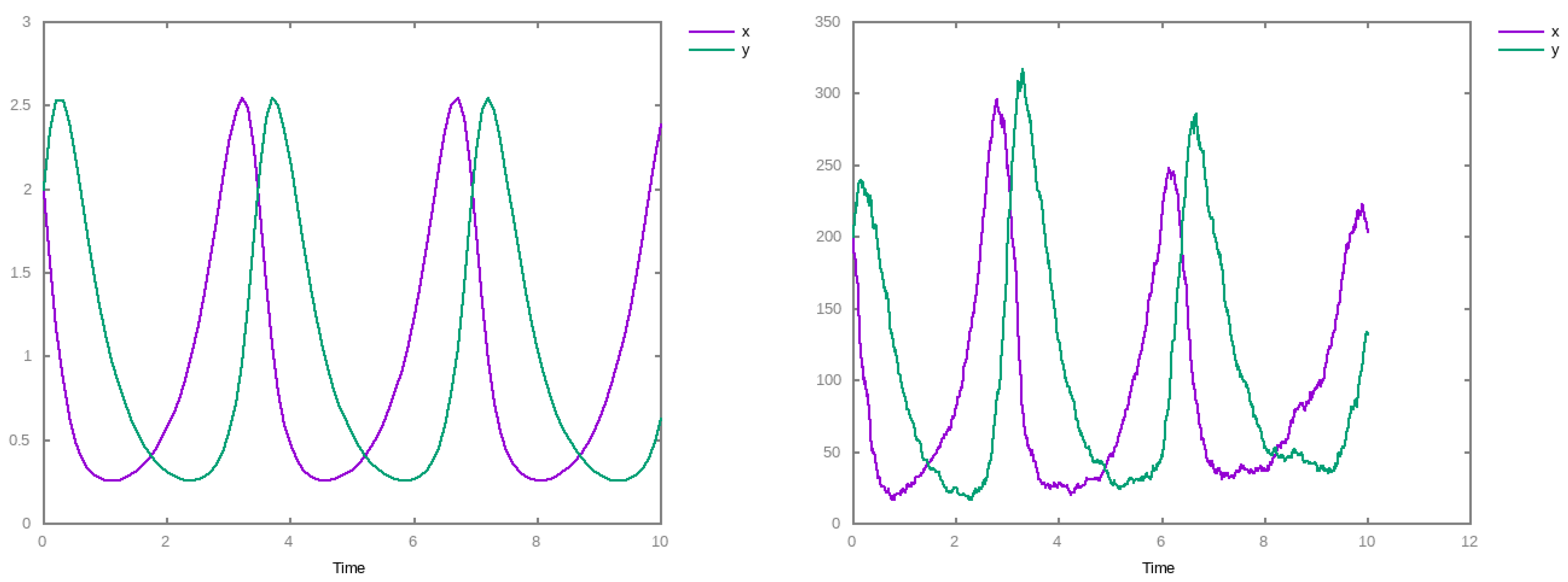
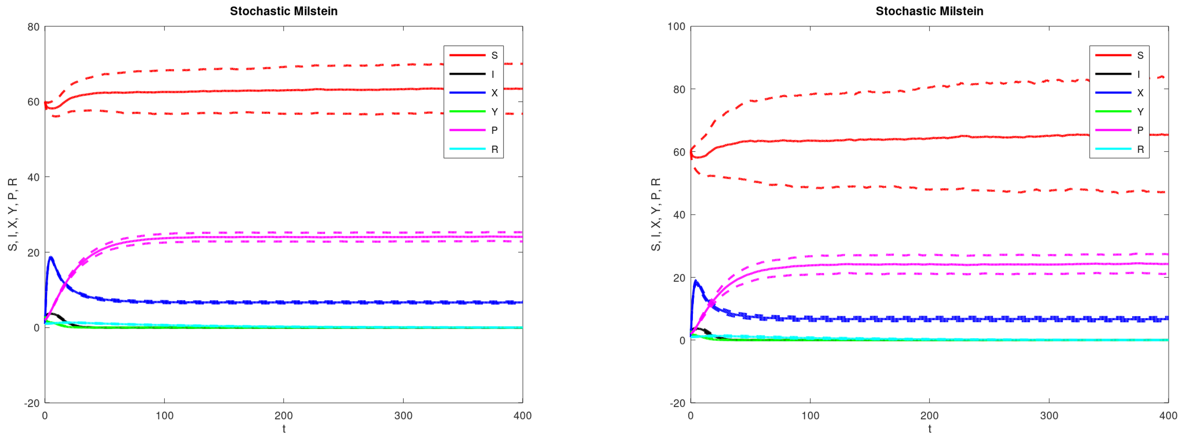
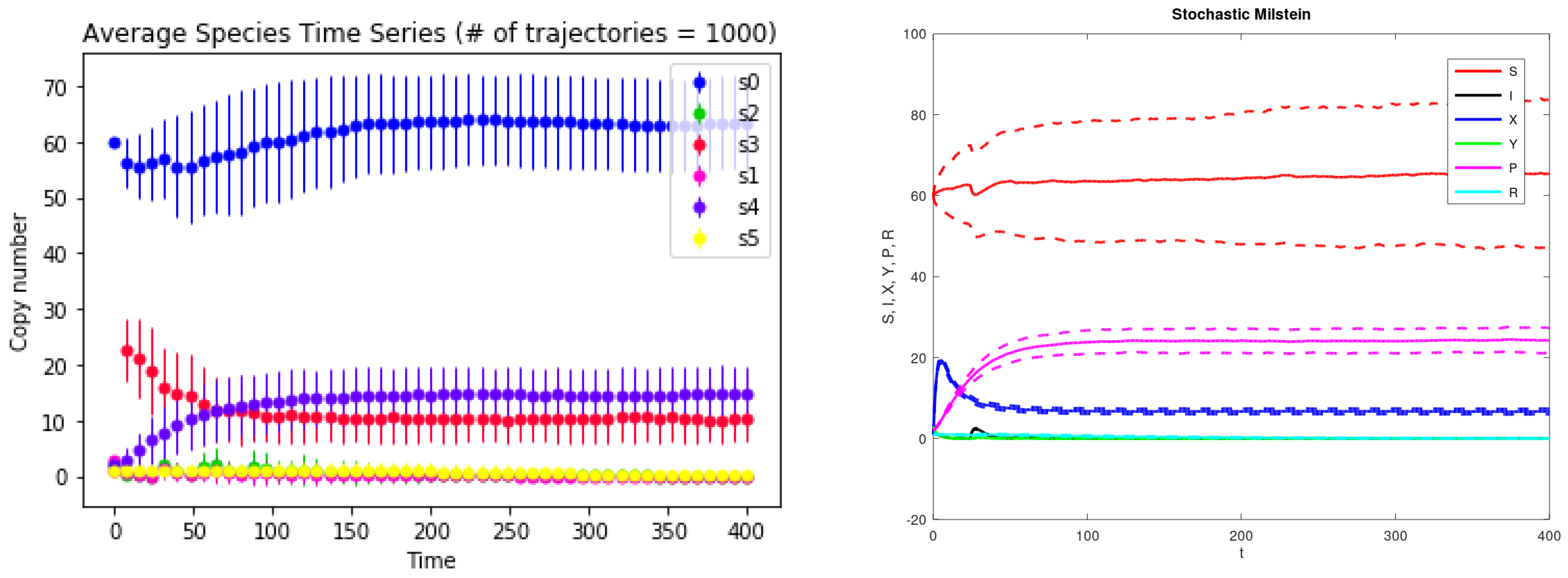
Numerical methods for ordinary differential equations can be modified for delay differential equations by integrating piece-wise over time intervals chosen such that they are multiples of the delays [55,56]. A very good numerical solver based on Runge–Kutta methods is given in [56]. In our numerical simulations we used the following values for our parameters: K = 63, $\beta$ = 0.01, ${\beta }_1$ = 0.01, $\alpha$ = 0.2, ${\alpha }_1$ = 0.1, $\mu$ = 0.01, m = 0.2974, $\gamma$ = 0.01, $\Lambda$ = 10, d = 0.2, $c_1$ = 0.05, $c_2$ = 0.05, $\delta$ = 0.05, ${\Lambda }_p$ = 0.4, ${\alpha }_3$ = 0.1 and ${\alpha }_4$ = 0.1. Additionally, we chose the following initial conditions: $S\left(0\right)=59.8478$, $I\left(0\right)=1.57612$, $X\left(0\right)=14.6247478$, $Y\left(0\right)=19.5$ and $P\left(0\right)=2$. We considered the values of the delays to be ${\tau }_1=24$ and ${\tau }_2=1$. The history for the delay equations is usually taken to be constant and equal to the initial values. However, if we consider the model in terms of reactions, the delayed reactions do not happen during the history, so we took the history to be equal to zero. The values of most the parameters were taken from [7] and those referring to the delays and the predator were from [10]. These are not implied to apply to specific plants, vectors and viruses. We were not able to find real values for many of the parameters. Even for the well studied maize streak virus, the model in [57], which uses the parameters presented in [58,59,60], some of the values are assumed.

For stochastic differential equations using Ito calculus, two common methods are the Euler–Murayama and Milstein methods [15]. Both can be easily modified to include delays in a similar way as for ordinary differential equations [61]. The SSA can be modified to include delays in the reactions by adding the corresponding delay to the time when the reaction happens [62,63].

For the deterministic ordinary differential equations we used an Euler method implemented in GNU octave [64]. For the stochastic differential equations the Milstein method was also implemented in octave. Both methods are first order. For the reaction-based method, we used the software stochPy [65], an open source program implemented in Python.

3. Results

The first simulation is of the SIR model given by differential Equation (1) and reaction (3). The values of the parameters were: $N=63,\beta =0.2$ and $\gamma =0.1$. The initial values were $S\left(0\right)=60,I\left(0\right)=2$ and $R\left(0\right)=1$. Figure 1 shows the deterministic simulation on the left and the SSA simulation on the right. For the SSA simulation, only the average values of the populations are plotted. For the values of the parameters used, the populations tended to the disease-free equilibrium for a large amount of time.

The next simulation was of the predator–prey model described by Equation (4) and reaction (5). The parameter values used were $p=1,r=1,b=1$ and $d=1$. The initial conditions were $X\left(0\right)=2$ and $Y\left(0\right)=2$. Figure 2 shows on the left the deterministic simulation and on the right the simulation using SSA. For the SSA simulation only the average values are plotted. Note that the deterministic solution is periodic but SSA is not quite periodic.

The next simulations were for the plant-virus model given by Equation (6) and reaction (7). The stochastic differential equations used were (8). The values of the parameters used in the simulations are in Table 1.

We did three simulations of the plant-virus model. The first one was with mass action kinetics and no delays. That is, ${\alpha }_1,{\alpha }_2,{\alpha }_3,{\alpha }_4,{\tau }_1$ and ${\tau }_2$ all being equal to zero. All the other parameters were as given in Table 1, with the exception of ${\sigma }_1$ to ${\sigma }_6$. An open question is how to determine the values of the $\sigma$s. We did one simulation of the deterministic model, one of the reaction model using the SSA and three of the stochastic differential equation model (8) using three different values of the $\sigma$, 0.01. 0.025 and 0.05. Figure 3 shows the results of the deterministic simulation on the left and of the SSA simulation on the right. The stochastic simulation shows the plots for the mean and the mean +/− standard deviation for 1000 realizations. Figure 4 shows the stochastic differential equation simulations results for the mean and the mean +/− one standard deviation for 1000 simulations with all $\sigma$s equal to 0.01 on the left and with the $\sigma$s equal to 0.025 on the right. Figure 5 shows on the left the mean and the mean +/− one standard deviation plots for the $\sigma$s equal to 0.05. From these figures we see that the $\sigma$s equal to 0.025 gives a stochastic effect that is important but does not overcome the deterministic part. The plots for the mean values of the stochastic simulations were taken for 1000 realizations since the results for 500 and 1000 realizations agree to at least three significant figures.

The next simulation for the plant-virus model is with Holling type 2 saturation kinetics and no delays. So ${\alpha }_1,\dots ,{\alpha }_4$ are nonzero with their values and the values of the other parameters given in Table 1 and ${\tau }_1={\tau }_2=0$. Figure 6 has the plots of the deterministic simulation. Figure 7 has the plots of simulations using the SSA (left) and stochastic differential equation s (right). For the SSA, the vertical lines represent the intervals [mean − 1 standard deviation, mean + 1 standard deviation]. For the stochastic differential equations plot the mean is given by the solid lines and the dashed lines give the mean +/− one standard deviation for 1000 realizations for the stochastic simulations. On the left for the SSA simulation and on the right for the stochastic differential equation run with $\sigma$s equal to 0.025.

The final simulation was for the plant-virus model with both saturation and delays. All the parametrer values are given in Table 1 and the delays were ${\tau }_1=24$ and ${\tau }_2=1$. Figure 8 has the plot of the deterministic simulation. Figure 9 has the plots of the mean and of the mean +/− one standard deviation for 1000 realizations for the stochastic simulations. On the left are the results for the SSA simulation, and the vertical lines represent the intervals (mean − 1 standard deviation, mean + 1 standard deviation). On the right are the plots for the stochastic differential equation run with $\sigma$ equal to 0.025. The solid lines represent the mean values and the dashed lines the mean +/− one standard deviation.

4. Discussions

The numerical simulations in all cases gave similar results for the differential equation, the stochastic differential and the reaction models. The differential equation simulations give one trajectory and do not take into account the variations in the populations and environment, or the errors in measurements of parameters. However, they are the easiest simulations to implement and the fastest. The stochastic differential equations include variations of the populations when multiplicative noise is added, as we did. By doing multiple simulations, they give the mean values and the standard deviations of the solutions, which are more realistic. However, there are other types of white noise and we need to estimate the size of the noise. The reaction model simulations using the Gillespie algorithm also give the means and standard deviations of the solutions when run for multiple simulations. It has a more solid theoretical base for small populations, and this is our case. Through both the stochastic differential equation method and the Gillespie algorithm there are some outcomes with different behavior than what comes from the deterministic method. For some realizations the disease may not disappear for very long time periods, and in future work it may be worth estimating the probability.

5. Conclusions

Mathematical population models based on differential equations give realistic results even when the populations are not very large. However, models based on biochemical reactions are more realistic. Models given in terms of reactions are usually easier to understand for biologists, ecologists and other specialists without backgrounds in mathematics. The stochastic simulation algorithm has solid theoretical backing for its use for small populations, and there is a wide variety of existing software implementing it. As with all stochastic simulations, there is the question of how many realizations to use. In our case we did one hundred and then one thousand realizations, and the results have at least three significant digits of agreement. The results for the stochastic differential equations depend on the type and magnitude of the white noise term, and it is usually not obvious which one should be used.

Even though from the first epidemic models it has been known that the models can be written in terms of biochemical reactions [66], their use and the use of Gillespie’s algorithm should be more frequent, since in epidemic models the populations are many times not very large and the continuity hypothesis is not justified. Second, this method is easy to implement and does not require one—as the stochastic differential method does—to decide on the type and magnitude of the white noise. There are many papers dealing with the use of Gillespie’s algorithm for epidemic models and others on using biochemical reactions and other methods. For example, in [67] the authors used a biochemical reactions formulation and cellular automata. In [68], the authors mentioned that epidemic models can be described as chemical reactions but then used a stochastic model based on binomial drawing for certain terms. In [31] the equivalent reactions for a SIR model are given. In some other papers the Gillespie algorithm was applied to variations of the SIR method [69,70,71]. Reference [72] presents continuous time Markov chain and stochastic differential equation models, including an SIR model and a four-population model for malaria. For this last model, the author approximated the branching process by working with the forward and backward Kolmogorov equations. In [70] the model used was an SEIR (Susceptible, Exposed, Infectious, Recovered) with added numbers of patients hospitalized and killed regarding Ebola. To the best of my knowledge, the publications about the applications of the Gillespie algorithm to epidemic models do not include models with saturation interaction terms, particularly with Holling type 2 functionals, or epidemic models with discrete delays; they also do not involve plant diseases caused bv viruses and spread by vectors. The comparison of the results for the model using stochastic equation simulations with different sizes for the white noise is also new. Future work will include applying the application to more complex models and to models with time varying rates.

References

1. Scholthof, K.B.G.; Adkins, S.; Czosnek, H.; Palukaitis, P.; Jacquot, E.; Hohn, T.; Hohn, B.; Saunders, K.; Candresse, T.; Ahlquist, P.; et al. Top 10 plant viruses in molecular plant pathology. Mol. Plant Pathol. 2011, 12, 938–954. [Google Scholar] [CrossRef] [PubMed]
2. Fereres, A. Insect vectors as drivers of plant virus emergence. Curr. Opin. Virol. 2015, 10, 42–46. [Google Scholar] [CrossRef] [Green Version]
3. Jeger, M.; Van Den Bosch, F.; Madden, L.; Holt, J. A model for analysing plant-virus transmission characteristics and epidemic development. Math. Med. Biol. A J. IMA 1998, 15, 1–18. [Google Scholar] [CrossRef]
4. Jeger, M.; Holt, J.; Van Den Bosch, F.; Madden, L. Epidemiology of insect-transmitted plant viruses: Modelling disease dynamics and control interventions. Physiol. Entomol. 2004, 29, 291–304. [Google Scholar] [CrossRef]
5. Van Maanen, A.; Xu, X.M. Modelling plant disease epidemics. Eur. J. Plant Pathol. 2003, 109, 669–682. [Google Scholar] [CrossRef]
6. Anguelov, R.; Lubuma, J.; Dumont, Y. Mathematical analysis of vector-borne diseases on plants. In Proceedings of the 2012 IEEE 4th International Symposium on Plant Growth Modeling, Simulation, Visualization and Applications, Shanghai, China, 31 October–3 November 2012; pp. 22–29. [Google Scholar]
7. Shi, R.; Zhao, H.; Tang, S. Global dynamic analysis of a vector-borne plant disease model. Adv. Differ. Equ. 2014, 2014, 59. [Google Scholar] [CrossRef] [Green Version]
8. Meng, X.; Li, Z. The dynamics of plant disease models with continuous and impulsive cultural control strategies. J. Theor. Biol. 2010, 266, 29–40. [Google Scholar] [CrossRef]
9. Al Basir, F.; Adhurya, S.; Banerjee, M.; Venturino, E.; Ray, S. Modelling the effect of incubation and latent periods on the dynamics of vector-borne plant viral diseases. Bull. Math. Biol. 2020, 82, 1–22. [Google Scholar] [CrossRef]
10. Jackson, M.; Chen-Charpentier, B.M. Modeling plant virus propagation with delays. J. Comput. Appl. Math. 2017, 309, 611–621. [Google Scholar] [CrossRef]
11. Jackson, M.; Chen-Charpentier, B.M. A model of biological control of plant virus propagation with delays. J. Comput. Appl. Math. 2018, 330, 855–865. [Google Scholar] [CrossRef]
12. Chen-Charpentier, B.M.; Jackson, M. Direct and indirect optimal control applied to plant virus propagation with seasonality and delays. J. Comput. Appl. Math. 2020, 380, 112983. [Google Scholar] [CrossRef]
13. Zhang, T.; Meng, X.; Song, Y.; Li, Z. Dynamical analysis of delayed plant disease models with continuous or impulsive cultural control strategies. Abstr. Appl. Anal. 2012, 2012. [Google Scholar] [CrossRef]
14. Al Basir, F.; Takeuchi, Y.; Ray, S. Dynamics of a delayed plant disease model with Beddington-DeAngelis disease transmission. Math. Biosci. Eng. 2021, 18, 583–599. [Google Scholar] [CrossRef] [PubMed]
15. Kloeden, P.E.; Platen, E. Numerical Solution of Stochastic Differential Equations; Springer Science & Business Media: Berlin/Heidelberg, Germany, 2013; Volume 23. [Google Scholar]
16. Evans, L.C. An Introduction to Stochastic Differential Equations; American Mathematical Soc.: Providence, RI, USA, 2012; Volume 82. [Google Scholar]
17. Ghanem, R.; Spanos, P.D. Polynomial Chaos in Stochastic Finite Elements. J. Appl. Mech. 1990, 57, 197–202. [Google Scholar] [CrossRef]
18. Xiu, D.; Karniadakis, G.E. The Wiener–Askey polynomial chaos for stochastic differential equations. SIAM J. Sci. Comput. 2002, 24, 619–644. [Google Scholar] [CrossRef]
19. Gibson, G.J. Markov chain Monte Carlo methods for fitting spatiotemporal stochastic models in plant epidemiology. J. R. Stat. Soc. Ser. C Appl. Stat. 1997, 46, 215–233. [Google Scholar] [CrossRef]
20. Keeling, M.J.; Ross, J.V. On methods for studying stochastic disease dynamics. J. R. Soc. Interface 2008, 5, 171–181. [Google Scholar] [CrossRef] [Green Version]
21. Qi, H.; Meng, X.; Chang, Z. Markov semigroup approach to the analysis of a nonlinear stochastic plant disease model. Electron. J. Differ. Equ. 2019, 2019, 1–19. [Google Scholar]
22. Stollenwerk, N.; Briggs, K.M. Master equation solution of a plant disease model. Phys. Lett. A 2000, 274, 84–91. [Google Scholar] [CrossRef]
23. Gillespie, D.T. Exact stochastic simulation of coupled chemical reactions. J. Phys. Chem. 1977, 81, 2340–2361. [Google Scholar] [CrossRef]
24. Cao, Y.; Gillespie, D.T.; Petzold, L.R. Efficient step size selection for the tau-leaping simulation method. J. Chem. Phys. 2006, 124, 044109. [Google Scholar] [CrossRef]
25. Hemberg, M.; Yaliraki, S.N.; Barahona, M. Stochastic kinetics of viral capsid assembly based on detailed protein structures. Biophys. J. 2006, 90, 3029–3042. [Google Scholar] [CrossRef] [Green Version]
26. Perlmutter, J.D.; Hagan, M.F. Mechanisms of virus assembly. Annu. Rev. Phys. Chem. 2015, 66, 217–239. [Google Scholar] [CrossRef] [PubMed] [Green Version]
27. Allen, L. An Introduction to Mathematical Biology; Pearson-Prentice Hall: Upper Saddle River, NJ, USA, 2007. [Google Scholar]
28. Gagniuc, P.A. Markov Chains: From Theory to Implementation and Experimentation; John Wiley & Sons: Hoboken, NJ, USA, 2017. [Google Scholar]
29. Holling, C. The Components of Predation as Revealed by a Study of Small Mammal Predation of the European Pine Sawfly. Can. Entomol. 1959, 91, 293–320. [Google Scholar] [CrossRef]
30. Fages, F.; Gay, S.; Soliman, S. Inferring reaction systems from ordinary differential equations. Theor. Comput. Sci. 2015, 599, 64–78. [Google Scholar] [CrossRef]
31. Simon, C.M. The SIR dynamic model of infectious disease transmission and its analogy with chemical kinetics. PeerJ Phys. Chem. 2020, 2, e14. [Google Scholar] [CrossRef]
32. Keeling, M.J.; Rohani, P. Modeling Infectious Diseases in Humans and Animals; Princeton University Press: Princeton, NJ, USA, 2011. [Google Scholar]
33. Fages, F.; Soliman, S. On robustness computation and optimization in BIOCHAM-4. In Proceedings of the International Conference on Computational Methods in Systems Biology, Brno, Czech Republic, 12–14 September 2018; Springer: Berlin/Heidelberg, Germany, 2018; pp. 292–299. [Google Scholar]
34. Ermentrout, B. Simulating, Analyzing, and Animating Dynamical Systems: A Guide to XPPAUT for Researchers and Students; Siam: Philadelphia, PA, USA, 2002; Volume 14. [Google Scholar]
35. Gómez, H.F.; Hucka, M.; Keating, S.M.; Nudelman, G.; Iber, D.; Sealfon, S.C. Moccasin: Converting matlab ode models to sbml. Bioinformatics 2016, 32, 1905–1906. [Google Scholar] [CrossRef] [PubMed] [Green Version]
36. Hucka, M.; Finney, A.; Sauro, H.M.; Bolouri, H.; Doyle, J.C.; Kitano, H.; Arkin, A.P.; Bornstein, B.J.; Bray, D.; Cornish-Bowden, A.; et al. The systems biology markup language (SBML): A medium for representation and exchange of biochemical network models. Bioinformatics 2003, 19, 524–531. [Google Scholar] [CrossRef]
37. Soong, T.T. Random Differential Equations in Science and Engineering; Academic Press: New York, NY, USA, 1973. [Google Scholar]
38. Pinsky, M.; Karlin, S. An Introduction to Stochastic Modeling; Academic Press: Burlington, MA, USA, 2010. [Google Scholar]
39. Allen, L.J. An Introduction to Stochastic Processes with Applications to Biology; CRC Press: Hoboken, NJ, USA, 2010. [Google Scholar]
40. Oksendal, B. Stochastic Differential Equations: An Introduction with Applications; Springer Science & Business Media: Berlin/Heidelberg, Germany, 2013. [Google Scholar]
41. McQuarrie, D.A. Stochastic approach to chemical kinetics. J. Appl. Probab. 1967, 4, 413–478. [Google Scholar] [CrossRef]
42. Van Kampen, N.G. Stochastic Processes in Physics and Chemistry; Elsevier: Amsterdam, The Netherlands, 1992; Volume 1. [Google Scholar]
43. Gillespie, D.T. Stochastic Simulation of Chemical Kinetics. Annu. Rev. Phys. Chem. 2007, 58, 35–55. [Google Scholar] [CrossRef] [PubMed]
44. Weber, M.F.; Frey, E. Master equations and the theory of stochastic path integrals. Rep. Prog. Phys. 2017, 80, 046601. [Google Scholar] [CrossRef] [PubMed] [Green Version]
45. Gibson, M.A.; Bruck, J. Efficient exact stochastic simulation of chemical systems with many species and many channels. J. Phys. Chem. A 2000, 104, 1876–1889. [Google Scholar] [CrossRef]
46. Van Gend, C.; Kummer, U. STODE-automatic stochastic simulation of systems described by differential equations. In Proceedings of the 2nd International Conference on Systems Biology, Pasadena, CA, USA, 4–7 November 2001; Volume 326, p. 333. [Google Scholar]
47. COmplex PAthway SImulator (COPASI). Available online: http://copasi.org/ (accessed on 12 December 2020).
48. Higham, D.J. Modeling and Simulating Chemical Reactions. SIAM Rev. 2008, 50, 347–368. [Google Scholar] [CrossRef] [Green Version]
49. Allen, E. Modeling with Itô Stochastic Differential Equations; Springer: Berlin/Heidelberg, Germany, 2007; Volume 22. [Google Scholar]
50. Gray, A.; Greenhalgh, D.; Hu, L.; Mao, X.; Pan, J. A stochastic differential equation SIS epidemic model. SIAM J. Appl. Math. 2011, 71, 876–902. [Google Scholar] [CrossRef] [Green Version]
51. Zhao, Y.; Jiang, D.; Mao, X.; Gray, A. The threshold of a stochastic SIRS epidemic model in a population with varying size. Discret. Contin. Dyn. Syst. Ser. B 2015, 20, 1277–1295. [Google Scholar] [CrossRef] [Green Version]
52. Zhu, L.; Hu, H. A stochastic SIR epidemic model with density dependent birth rate. Adv. Differ. Equ. 2015, 2015, 330. [Google Scholar] [CrossRef] [Green Version]
53. Rao, F. Dynamics analysis of a stochastic SIR epidemic model. Abstr. Appl. Anal. 2014, 2014, 356013. [Google Scholar] [CrossRef]
54. Chang, Z.; Meng, X.; Zhang, T. A new way of investigating the asymptotic behaviour of a stochastic SIS system with multiplicative noise. Appl. Math. Lett. 2019, 87, 80–86. [Google Scholar] [CrossRef]
55. Bellen, A.; Zennaro, M. Numerical Methods for Delay Differential Equations; Oxford University Press: Oxford, UK, 2013. [Google Scholar]
56. Shampine, L.F.; Thompson, S.; Kierzenka, J. Solving Delay Differential Equations with dde23. 2000. Available online: http://www.runet.edu/~thompson/webddes/tutorial.pdf (accessed on 12 December 2020).
57. Alemneh, H.T.; Makinde, O.D.; Theuri, D.M. Optimal Control Model and Cost Effectiveness Analysis of Maize Streak Virus Pathogen Interaction with Pest Invasion in Maize Plant. Egypt. J. Basic Appl. Sci. 2020, 7, 180–193. [Google Scholar] [CrossRef]
58. Bosque-Pérez, N.A. Eight decades of maize streak virus research. Virus Res. 2000, 71, 107–121. [Google Scholar] [CrossRef]
59. Magenya, O.; Mueke, J.; Omwega, C. Significance and transmission of maize streak virus disease in Africa and options for management: A review. Afr. J. Biotechnol. 2008, 7, 4897–4910. [Google Scholar]
60. Alemneh, H.T.; Makinde, O.D.; Mwangi Theuri, D. Ecoepidemiological Model and Analysis of MSV Disease Transmission Dynamics in Maize Plant. Int. J. Math. Math. Sci. 2019, 2019. [Google Scholar] [CrossRef] [Green Version]
61. Mao, X.; Sabanis, S. Numerical solutions of stochastic di erential delay equations under local Lipschitz condition. J. Comput. Appl. Math. 2003, 151, 215–227. [Google Scholar] [CrossRef] [Green Version]
62. Barrio, M.; Burrage, K.; Leier, A.; Tian, T. Oscillatory Regulation of Hes1: Discrete Stochastic Delay Modelling and Simulation. PLoS Comput. Biol. 2006, 2, e117. [Google Scholar] [CrossRef] [PubMed] [Green Version]
63. Barbuti, R.; Caravagna, G.; Milazzo, P.; Maggiolo-Schettini, A. On the Interpretation of Delays in Delay Stochastic Simulation of Biological Systems. Electron. Proc. Theor. Comput. Sci. 2009, 6, 17–29. [Google Scholar] [CrossRef] [Green Version]
64. GNU. GNU Octave. Library Catalog. Available online: www.gnu.org (accessed on 12 December 2020).
65. Maarleveld, T.R.; Olivier, B.G.; Bruggeman, F.J. StochPy: A Comprehensive, User-Friendly Tool for Simulating Stochastic Biological Processes. PLoS ONE 2013, 8, e79345. [Google Scholar] [CrossRef] [PubMed] [Green Version]
66. Kermack, W.O.; McKendrick, A.G. A contribution to the mathematical theory of epidemics. Proc. R. Soc. Lond. Ser. A Contain. Pap. Math. Phys. Character 1927, 115, 700–721. [Google Scholar]
67. Mondal, S.; Mukherjee, S.; Bagchi, B. Mathematical modeling and cellular automata simulation of infectious disease dynamics: Applications to the understanding of herd immunity. J. Chem. Phys. 2020, 153, 114119. [Google Scholar] [CrossRef]
68. Cummings, D.A.; Lessler, J. Infectious disease dynamics. In Infectious Disease Epidemiology: Theory and Practice; Nelson, K.E., Masters Williams, C., Eds.; Jones & Bartlett Publishers: Burlington, MA, USA, 2014; pp. 131–166. [Google Scholar]
69. Funk, S.; Salathé, M.; Jansen, V.A. Modelling the influence of human behaviour on the spread of infectious diseases: A review. J. R. Soc. Interface 2010, 7, 1247–1256. [Google Scholar] [CrossRef]
70. Rivers, C.M.; Lofgren, E.T.; Marathe, M.; Eubank, S.; Lewis, B.L. Modeling the impact of interventions on an epidemic of Ebola in Sierra Leone and Liberia. PLoS Curr. 2014, 6. [Google Scholar] [CrossRef]
71. Begon, M.; Bennett, M.; Bowers, R.G.; French, N.P.; Hazel, S.; Turner, J. A clarification of transmission terms in host-microparasite models: Numbers, densities and areas. Epidemiol. Infect. 2002, 129, 147–153. [Google Scholar] [CrossRef] [PubMed]
72. Allen, L.J. A primer on stochastic epidemic models: Formulation, numerical simulation, and analysis. Infect. Dis. Model. 2017, 2, 128–142. [Google Scholar] [CrossRef] [PubMed]
Figure 1. Simulation of susceptibles (S), infectives (I) and recovereds (R) (SIR) model. (Left) deterministic. (Right) Stochastic simulation algorithm (SSA); only the average values are shown.
Mathematics 09 00456 g001
Figure 2. Simulation of the predator–prey model. (Left) deterministic. (Right) SSA; only the average values are shown.
Mathematics 09 00456 g002
Figure 3. Plots for the virus plant model with mass action interactions and no delays. (Left) deterministic. (Right) SSA with only the average values included.
Mathematics 09 00456 g003
Figure 4. Plots for the plant-virus model with mass action interactions and no delays using the stochastic differential equations model. The solid lines are the mean values, and the dashed lines are the mean value plus or minus one standard deviation. (Left) σ s equal to 0.01. (Right) σ s equal to 0.025.
Mathematics 09 00456 g004
Figure 5. Plots for the plant-virus model for mass action interactions and no delays using the stochastic differential model. The solid lines are the mean values, and the dashed lines are the mean values +/− one standard deviation. The σ s are equal to 0.05.
Mathematics 09 00456 g005
Figure 6. Plots for the virus plant model with saturations and no delays for the deterministic model.
Mathematics 09 00456 g006
Figure 7. Plots for virus plant models with saturation and no delays. (Left) SSA; the vertical lines denote the intervals (mean − 1 standard deviation, mean + 1 standard deviation). (Right) Stochastic differential equations simulation—mean values (solid lines) and mean values +/− 1 standard deviation (dashed lines).
Mathematics 09 00456 g007
Figure 8. Plots for the virus plant model with saturations and delays for the deterministic model.
Mathematics 09 00456 g008
Figure 9. Plots for mean values and the mean values +/− 1 standard deviation for the virus plant model with saturation and delays. (Left) SSA with the vertical lines giving the intervals (mean − 1 standard deviation, mean + 1 standard deviation). (Right) Stochastic differential equations with the solid lines giving the mean values and the dashed lines the means +/− 1 standard deviation.
Mathematics 09 00456 g009