Improving the Gridshells’ Regularity by Using Evolutionary Techniques

Abstract

Designing and optimizing gridshell structures have been very attractive problems in the last decades. In this work, two indexes are introduced as “length ratio” and “shape ratio” to measure the regularity of a gridshell and are compared to the existing indexes in the literature. Two evolutionary techniques, genetic algorithm (GA) and particle swarm optimization (PSO) method, are utilized to improve the gridshells’ regularity by using the indexes. An approach is presented to generate the initial gridshells for a given surface in MATLAB. The two methods are implemented in MATLAB and compared on three benchmarks with different Gaussian curvatures. For each grid, both triangular and quadrangular meshes are generated. Experimental results show that the regularity of some gridshell is improved more than 50%, the regularity of quadrangular gridshells can be improved more than the regularity of triangular gridshells on the same surfaces, and there may be some relationship between Gaussian curvature of a surface and the improvement percentage of generated gridshells on it. Moreover, it is seen that PSO technique outperforms GA technique slightly in almost all the considered test problems. Finally, the Dolan–Moré performance profile is produced to compare the two methods according to running times.

1. Introduction

Gridshells which are also called lattice shells or reticulated shells are generally defined as structures with the shape and rigidity of a double curvature shell consisting of a grid not a continuous surface [1]. Although gridshells come to several forms, they are usually designed with triangular, quadrilateral, or hexagonal faces (or grid cells) [1,2,3,4,5,6,7,8,9,10]. Forming and optimizing gridshell structures have been very attractive problems in the past decades. Several approaches, such as inversion method [1], dynamic relaxation [2,4,11], force density method [3,12], and so forth [10,13], have been studied so far in the literature to address the problem of forming a grid shell structure. Moreover, various techniques from gradient-based to evolutionary methods have been employed for optimization of gridshells taking into account various aspects of a gridshell such as economic, structural, or aesthetic [11,12,13,14,15,16,17,18]. The focus of this work is on the optimization problem, and it is assumed that the initial forms of the desired gridshells are given.

Bouhaya et al. [1] coupled genetic algorithms with a geometric technique, which is called compass method, to present a novel approach for generating elastic gridshells on an imposed shape with boundary conditions. The authors used three benchmarks with different Gaussian curvature to illustrate the proposed technique. These benchmarks are also employed in the present work for generating the numerical results as they contain a variety of conditions with different Gaussian curvatures. Richardson et al. [11] presented a two-phase design technique. Using a multi-objective genetic algorithm, Winslow et al. [17] established a design tool for synthesis of optimal gridshell structures taking into account two or more load cases such as wind load. Feng et al. [5] considered three categories of indexes including mechanical, geometry, and economic criteria for optimization of free-form cable-braced gridshells. Focusing on triangular gridshells and optimization over a free-form surface, Wang et al. [16] presented a framework to generate gridshells.

We note that usually the researchers have taken into account the structural aspects of gridshells in optimization phase and less attention has been heeded to improvement of the gridshells’ regularity while the later can affect directly on the economy and aesthetic indexes. In fact, improving the regularity of a gridshell may lead to decreasing the number of different elements’ types as well as enhancing the aesthetic aspect of the desired grids. Hence, in this work, improvement of the regularity of gridshells is considered as the main aim. To this end, two indexes are introduced to measure the regularity of a gridshell. The indexes are called “length ratio” and “shape ratio” and defined as the standard deviation of all the elements’ lengths and all the inner angles in the gridshells’ faces, respectively. There are a few studies in the literature which have worked on improving the regularity of gridshells. In fact, to the best of our knowledge, this is the first time that these two indexes are introduced for measuring the free-form gridshells’ regularity. Considering the geodesic domes, Nooshin and his coworkers in [19] have proposed some measures for making the regularity of such structures quantifiable. Here, we compare our introduced indexes with the proposed ones in [19] on some benchmark for illustrating the practical efficiency of the introduced indexes in this work.

It is noted that although gradient-based techniques guarantee a superior convergence rate for the cases with a few number of design variables, in the cases with many design variables, generally, evolutionary methods work more appropriately. This is why we employ evolutionary techniques in this work. Among the evolutionary techniques, genetic algorithms (GAs) have been used the most in optimization of gridshells [1,3,5,8,10,11,13,14,15,16,17,18]. Another well-known evolutionary method is particle swarm optimization (PSO) to which less attention has been paid for improving the gridshell structures so far. However, it is a very powerful technique and has been applied to many other optimization problems [20,21,22,23,24,25,26,27]. Thus, these two techniques are considered in the present work.

We first present an approach, Algorithm 1, for generating initial triangular and quadrangular gridshells in MATLAB. Then, it is explained how the nodal positions in a given grid can be represented as birds (or particles) in PSO technique and as chromosomes in GA, and how these techniques can be used to improve the regularity of gridshells by bettering the nodal positions. We introduce two indexes to make the gridshells’ regularity quantifiable and use them in the improvement process. Moreover, providing the numerical results, it is illustrated that our introduced indexes are practically more efficient than the existing indexes in the literature. In addition, the performances of GA and PSO techniques are compared through experimental results generated on eighteen test problems by which several interesting observations are obtained. Finally, we produce the Dolan and Moré performance profile [28] to have a more intuitive comparison between GA and PSO technique based on running times.

The rest of this work is organized as follows. Section 2 presents an algorithm to generate the initial gridshells for a given surface in MATLAB, explains briefly the GA and PSO techniques stage by stage, describes how these techniques can be used for improving the gridshells’ regularity, and moreover provides the mathematical model for the problem. In Section 3, first our introduced indexes are compared to two existing ones in the literature on some benchmark, and then the performances of GA and PSO techniques are compared on three benchmarks. Finally, Section 4 provides the concluding remarks and some directions for the future works.

2. Main Block

Here, an approach, Algorithm 1, is presented to generate initial gridshells. Then, we describe the genetic algorithm (GA) and particle swarm optimization (PSO) technique briefly for making it more convenient to read this work without having previous knowledge of these methods. Next, two indexes are introduced for making the gridshells’ regularity quantifiable, and finally the mathematical model of the problem is provided.

2.1. Generating An Initial Gridshell

There are several different approaches in the literature to generate an initial form of gridshell. Bouhaya et al. [1] used the compass method which is a geometric approach and allows creating a network of parallelograms on any surface. The authors then coupled the compass method with genetic algorithms to propose an optimization approach. In optimization of the cable-braced grid shells, Feng et al. [5] created the initial forms by translating the generatrix and directrix which allows the mesh to be parallelogram. The authors then proposed an optimization technique based on the usage of generatrix and directrix. Wang et al. [16] formed the surface model by using NURBS (non-uniform rational B-splines), then generated a set of uniformly distributed random points on the surface, and finally connected the points by using Delaunay-based triangularization to generate an initial triangular gridshell.

It is noted that usually the proposed optimization methods in the literature are based on some generating techniques for the initial form. However, the focus of this work is on the regularity improvement of a given gridshell without taking into account how the initial form is obtained, and hence the presented techniques here can be used for improving the regularity of any given initial form of a gridshell which is given as two sets. A set with the (Cartesian) coordinates of nodes (or vertices), which is denoted by V here, and another set which shows the faces in the grid and is denoted by F here. In fact, F is a matrix, each row of which states which vertices form the corresponding face (or grid cell). Having the set V of the initial gridshell, the proposed approach here can be employed to improve the regularity of the gridshell by bettering the positions of the nodes without making any change in the matrix F. Moreover, one can add some restrictions such as fixing the position of some nodes to the improvement process.

In this work, for convenience and not being involved in the complication of generating the initial gridshells which is not of our focus, it is assumed that the given gridshell is based on a surface F(x, y, z) = 0. In this way, to keep the nodes (vertices) on the desired surface, the improvement process is made on the first two coordinates of the vertices, i.e., x and y, and the third coordinate is always obtained by using the surface equation. Any way, we observe that the detailed approach here can be employed for any given initial gridshell.

Another aspect to notice is that although gridshells with the triangular to hexagonal grid cells have been studied in the literature, triangular grids are the most widely used in reality as they can describe any free-form shape [16]. In addition, as the triangular gridshells have less economic advantages in construction than the equivalent structures built of quadrilateral grids, many researchers have studied quadrangular gridshells [5]. As a result, one can say that triangular and quadrangular gridshells are the most important cases, and hence the focus of this work is on these two groups of gridshells.

Given a surface F (x, y, z) = 0, to build an initial gridshell, usually some uniformly distributed random points are generated on the surface and then those points are connected to construct the triangular or quadrangular grid cells. However, as our main object here is to improve the regularity of the initial gridshells, we consider the equidistant points on the surface at the beginning which is the most regular initial case, and then we see that it can be still improved by using our introduced indexes. After generating the equidistant points on the surface, we use a very nice function in MATLAB, i.e., surf2patch(), to transform the coordinates (x, y, z) to two matrices V and F. However, it is possible to have duplicate vertices in V as any vertex in a grid cell may belong to some other cells as well. Hence, there may also be some duplicativeness in matrix F which should be removed.

This way, we present the following algorithm which generates both triangular and quadrangular initial gridshells (matrices F, faces, and V, vertices) for any given surface F(x, y, z) = 0.

Some explanations are given in Appendix A Section on the used MATLAB functions and commands in Algorithm 1. We note that Algorithm 1 works with any generated set of points in Step 1 including the uniformly distributed random points or the equidistant points on the surface. However, in our usage of this algorithm, we generate the equidistant points on x−axis and y−axis (and then the third coordinates of the points are determined by using the given surface F(x, y, z) = 0) rather than the randomly generated points. This is only to have the most regular initial gridshell.

Algorithm 1. Generating initial triangular or quadrangular gridshells (matrices F and V) for a given surface F(x, y, z) = 0 with some specified domain (in MATLAB)

Step 1. Generating some points on the surface in the domain. This way, we obtain three matrices X, Y, and Z including the coordinates of the points. Set ind (0 for triangular or 1 for quadrangular case).

Step 2. Determine the matrices F, faces, and V, vertices, as follows.     if ind     [F, V] = surf2patch(X, Y, Z)     else,     [F, V] = surf2patch(X, Y, Z, ‘triangles’).

Step 3. Remove the redundant vertices in matrices F and V as follows.

[V, ∼, I] = unique (V, ‘rows’);

F = I(F);

2.2. Genetic Algorithm

Here, we explain briefly the genetic algorithm (GA) to eliminate the need for previous knowledge of this technique for the readers. The genetic algorithm (GA) is an iterative search method which relies on bio-inspired operators such as selection, crossover, and mutation. This technique was developed by Holland [29] and contains six main stages explained below. It is noted that our main aim is not proposing an improved GA or tuning the best parameters of GAs on the desired problems but rather is to show how this technique can be employed to improve the gridshells’ regularity by using our introduced indexes in MATLAB. By the way, we tested some of the very common values for the parameters in GA taken from the literature, and then considered the best ones in our primary generated numerical results.

(1) Generating an initial population: Based on Darwinism, in this technique it is always assumed that there is an initial population of individuals which can change partially in each generation (iteration in the algorithm) according to the fitness (or cost) function. In fact, in each iteration the weak individuals are normally removed and instead some new stronger offspring are added to the population according to the crossover and mutation processes. We note that the number of individuals in each generation are the same as the number of individuals in the initial population. To generate an initial population, usually some random solutions are generated within a certain reasonable domain. Moreover, each solution, which is a member of the initial population, should be represented as a string (vector or matrix), which is called chromosome in this technique.

It is noted that although both matrices F and V are required to draw (or drive) the desired gridshells, the matrix F does not change during the improvement process, and we only need to improve the nodal positions according to the desired cost function. Hence, only the matrix V is improved. Moreover, with the first two coordinates of each vertex, i.e., x and y, the third coordinate can be obtained by using the given surface, that is F (x, y, z) = 0. Therefore, in this work, the first two columns of the initially generated matrix V are considered as a basic solution and denoted by V_new. Then, a population of N_pop individuals is randomly generated between V_new − t and V_new + t as the initial population, where t is a tolerance. As the initially generated matrix F, which shows the faces in the gridshell, does not change in the improvement process, the same matrix is used to evaluate every individual in the population.

(2) Evaluating each solution: An important part in every improvement process is determining the fitness function (in the case of maximizing) or cost function (in the case of minimizing), and then adopting it to the process. After generating the initial population, every individual is evaluated. The newly obtained solutions in crossover and mutation processes are also evaluated.

Then, usually in the merging stage, all the solutions are sorted and the weak ones are removed. Here, the cost function is considered as one of the presented indexes or their combination. More details on the cost function in our work is given in Section 2.5.

(3) Parent selection: In genetic algorithm, two current solutions (called parents) are selected in order to create two new solutions (called offspring or children) in crossover stage. There are various methods to select parents among which the random selection, tournament selection, and roulette wheel selection are the most used [30,31,32]. Here, we use the roulette wheel selection method. For improving this method, we first generate a vector of probability, i.e., P = (p₁, ···, p_Npop), based on the Boltzmann selection technique [33,34] and using a selection pressure β as follows.

$$\begin{gathered} \left(i\right) P=exp\left(-\beta \times C/C_{max}\right) \\ \left(ii\right) P=P/{{\displaystyle \sum }}_{j=1}^{N_{pop}}{p}_j \end{gathered}$$

(1)

where C is the vector of the solutions’ costs and ${\mathrm{C}}_{\max }$ is the cost of the worst solution in the current population. According to experimental results, to improve the convergence of GA technique, for each problem, we set the selection pressure β so that the summation of the first half of components in probability vector P stays between 0.7 and 0.8. This way, we obtain some probabilities whose summation is 1. Calculating the accumulated vector and generating a random number from zero to 1, the first component in the accumulated vector which is equal to or greater than this random number gives the desired parent. The crossover percentage in GA is usually considered between 0.5 and 1 [31]. Here, it is set to pc = 0.8. It is noted that in our primary numerical experiments on desired problems here, changing the crossover percentage from 0.7 to 0.9 led to a negligible change in the final results, and so the average of pc = 0.8 is considered. Therefore, as the number of parents should be even, in each iteration N_c = 2 × [pc × N_pop/2] parents are selected and the same number of offspring (children) are generated, where [•] is the nearest integer number to •.

(4) Crossover: This is an important operator in GA which mimics mating in biological populations. It propagates the good features from the current population to the next one leading to better fitness (or cost) value on average. There are several strategies to do the crossover including single point, double-point, uniform, and arithmetic crossover. Here, as the points can move continuously on the surface, we use the arithmetic crossover. In this way, we first generate a vector α of random numbers from the continuous uniform distribution, and then considering X1 and X2, the new children Y1 and Y2 are generated as follows.

$$Y_1={\alpha }_{.}\times X_1+{\left(1-\alpha \right)}_{.}\times X_2$$

(2)

$$Y_2={\alpha }_{.}\times X_2+{\left(1-\alpha \right)}_{.}\times X_1.$$

(3)

(5) Mutation: This operator allows for global search of the solution’s space, promoting the diversity in population characteristics. It also prohibits getting trapped in local minima. The mutation percentage in GA is usually chosen between 0.001 and 0.5 [31], and hence according to our primary generated numerical results pm = 0.3 is considered in this work. This way, in each generation (from the second generation), Nm = [pm × N_pop] of mutants are generated. Moreover, to generate a mutant, a mutation rate less than 0.1 is usually considered in GA [31,32]. Comparing the numerical results for different values 0.01, 0.02, ···, 0.08, we consider µ = 0.02 as mutation rate which determines the number of components (or genes) which are changed in the selected solution (or chromosome), and we do the mutation by using the standard normal distribution to change the values of the selected components in each solution. In fact, $\lceil \mathsf{\mu }\times N_v\rceil$ component are changed in the selected solution for mutation, where $N_{\vartheta }$ is the number of vertices in the gridshells and $\lceil •\rceil$ is the smallest integer number not less than •.

(6) Merging: After selecting parents, generating new children, and mutating some solutions, we merge all the current and newly obtained solutions leading to N_pop + N_c + N_m solutions. Then, as the number of solutions in each generation should be the same, all the solutions are sorted and arranged ascendingly according to the costs, and the first N_pop ones are selected as the next population.

We note that in GA the stages (3)–(6), explained above, are repeated until some considered stop criteria is satisfied.

Stop criteria. In fact, in all the iterative processes such as GA and PSO, the algorithm needs some stopping criteria. Some common stopping criteria used in the literature are: (i) stop by exceeding the given maximum number of iterations, (ii) stop when the improvement of solution in a given number of iterations is less than a given limit, (iii) stop when a satisfactory solution is determined, and (iv) stop when the cost function slope is almost zero. Here, for both GA and PSO, we consider a maximum number of M = 2000 iteration as the stop criterion.

2.3. Particle Swarm Optimization

Here, we explain briefly the particle swarm optimization (PSO) for the reader not being required to have any previous knowledge of this technique as well. This technique is also an iterative search method, inspired from social behavior, which was initially proposed by Kennedy and Eberhart [30]. There are four main stages in PSO explained as follows.

(1) Generating an initial population: Like GA, it is assumed that there is some initial population of individuals, called particles, in PSO. Usually, all the particles in PSO move from the current positions to some new positions based on the swarm intelligence in each iteration. Here, we consider the same initial population for PSO as the GA method. It is noted that each row in the matrix V_new, defined in Section 2.3, shows the position of a particle in the initial population and the matrix is updated whenever the position of the particles are changed. We note that the initially generated particles move toward the positions of the so-called Pbest and Gbest, explained below.

Thus, after generating the initial population, we need to evaluate them to determine Pbest and Gbest in the population.

(2) Velocity Updating: In this technique, the movement of each particle in every iteration is determined by its velocity. Let $x_i^k$ and $v_i^k$ respectively denote the position and velocity of particle i in the kth iteration in the search space. The velocity of particle i for the next iteration is calculated as follows.

$$v_i^{k+1}=w{v}_i^k+c_1{r}_1\left(Pbes{t}_i^k-x_i^k\right)+c_2{r}_2\left(Gbes{t}^k-x_i^k\right)$$

(4)

where w is the inertia factor which controls the flying dynamics, $c_1$ and $c_2$ are the acceleration factors for the experiences of Pbest and Gbest, respectively, ${\mathrm{r}}_1$ and ${\mathrm{r}}_2$ are random variables in the interval [0,1] which provide the ability of stochastic searching for PSO. The accelerating factors $c_1$ and $c_2$ compromise the trade-off between exploitation and exploration. It is noted that $Pbes{t}_i^k$ is the best experienced position for particle i until the kth iteration, and $Gbes{t}^k$ is the best experienced position among all the particles so far. We also note that the velocities for the particles in the initial population are set initially to be zero.

There are three parameters in Equation (4) which are w, $c_1$, and $c_2$. Many studies have been done so far to determine the best parameters for PSO technique. On the inertia weight, i.e., w, the studies show that a fixed w will not get to good results, and hence several techniques have been proposed in the literature by which w is lessened along with iteration times [26]. Some researchers suggested the interval [0.9,1.2] and some others the interval [0,1] for w [25,26,30]. Similarly, several researchers have studied the acceleration factors $c_1$ and $c_2$, and suggested different values for these factors. As our main aim is not tuning the best parameters for the PSO method in this area, we simply compared the four more common strategies taken from literature [26] numerically to select the best one. The strategies are (1) w = 1, wdamp = 0.999, $c_1=2$ and $c_2=2$, (2) w = 1, wdamp = 0.999, $c_1$ = 2.8 and $c_2$ = 1.3, (3) w = 1, wdamp = 0.999, $c_1$ = 1.49445 and $c_2$ = 1.49445 and (4) Letting φ₁ = 2.05, φ₂ = 2.05, φ = φ₁ + φ₂, and ξ = 2/(φ − 2 + $\sqrt{\mathsf{\phi }2-4\mathsf{\phi }}$), then we have w = ξ, $c_1$ = ξ × φ₁, and $c_2$ = ξ × φ₂. We note that in the first three strategies, the inertia weight is updated in each iteration by w = w.wdamp, and this is why wdamp is called the damping factor. It is also noted that the values of $c_1$ and $c_2$ in the strategies 3 and 4 are the same. We found the first strategy as the best among these four strategies for our desired problem, and hence we consider its parameters in this work.

We note that after updating velocities and before updating the particles’ positions, it is important to check if the velocities are within a pre-specified range. In fact, to avoid violent random walking and control the global exploration of the particles, some lower and upper speed limits for each particle are determined and when the velocity of a particle exceeds one of the limits, it is replaced with the related limit. These limits do not impact on the particle position, and only lessen the step size of velocity, and hence the limits control the particles’ moves and the aspects of exploration and exploitation [25,30]. Moreover, greater (smaller) speed limits lead to global (local) exploration [25,30]. The process of controlling velocity is called velocity clamping.

Although the movement of particles are controlled by velocity limits, sometimes even by using the lower limit of velocity, the new position of a particle is obtained out of the search area or feasible space. In fact, when the current position of a particle is close enough to the borders of the search area, according to the direction of velocity, even with small velocity, the new position of the particle will be out of the search area. This shows that in the next iterations, according to the inertia, this will happen again that the new position of the particle stays out of search space. Hence, to avoid such an event, the direction of velocity is changed to the opposite direction, that is its sign will be changed. This process is called “velocity mirror effect”.

(3) Position Updating: Unlike the genetic technique in which usually not all the members of the population are replaced with some new children in each iteration, in the PSO method, all the particles in the population move and change in each iteration. To do so, after calculating the velocity of the particle i, its position is updated as follows.

$$x_i^{k+1}=x_i^k+v_i^{k+1}$$

(5)

Apart from all the modifications and limits on the velocities, the new positions of some particles may be out of the search area. Hence, the updated positions should be checked for being within the allowed domain. If the position of a particle exceeds the lower or upper bounds, the position of the particle is replaced with the associated bound.

(4) Memory updating: In this technique, in each iteration, the position of every particle may change, and it is one of the differences between GA and PSO. Therefore, after updating the positions of the particles, we need to evaluate all the particles in order to check if it is required to update the P best and Gbest variables as they play an essential role in movement of the particles. However, it is not required to sort the particles after the evaluation process, and we only need to update the memory of P best and Gbest, if it is required. In this work, the same cost function is considered for both GA and PSO techniques.

The above-mentioned stages (2)–(4) in PSO are repeated until some considered stop criteria is satisfied. As stated in the previous section, we consider a maximum number of M = 2000 iteration as stop criteria for both GA and PSO in this work.

2.4. The Regularity Indexes

Here, we explain in more detail our introduced indexes, which are length ratio and shape ratio, as well as two similar indexes introduced in [19]. As the indexes introduced by Nooshin and his coworkers have been also called length and shape ratios, to make the four indexes distinguishable, we denote our length and shape ratios by OLR and OSR, respectively, and the introduced length and shape ratios by Nooshin and his coworkers by NLR and NSR, respectively. We recall that V is a matrix containing the position of all the vertices in Cartesian coordinates with no redundant vertices. In fact, V is an N_v × 3 matrix, where N_v is the number of vertices in the gridshell. Each row in V provides the Cartesian coordinates of a vertex in the grid, and the vertices are numbered in the order of appearance in V.

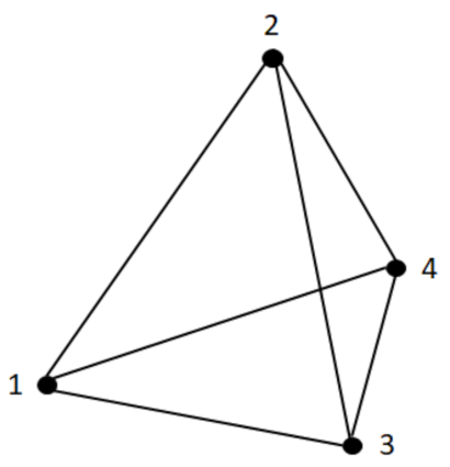
In the order of appearance in V. For instance, the vertex whose coordinates are given in the third row of V is numbered 3. The matrix F gives the vertices of each face. In fact, in a triangular (quadrangular) gridshell, F is an N_f × 3 (N_f × 4) matrix, where N_f is the number of faces in the grid. Each row in F shows which vertices are in the corresponding face. To have a better understanding, a simple grid (pyramid) is given in Figure 1. The matrices F and V for this figure are as follows.

$$\mathrm{V}=\left[\begin{array}{cccc}\mathbf{0}& \mathbf{0.65}& \mathbf{0}& \\ \mathbf{0.35}& \mathbf{0.45}& \mathbf{0.7}& \\ \mathbf{0.35}& \mathbf{0}& & \mathbf{0}\\ \mathbf{0.75}& \mathbf{0.65}& \mathbf{0}& \end{array}\right]\mathrm{F}=\left[\begin{array}{ccc}\mathbf{1}& \mathbf{2}& \mathbf{3}\\ \mathbf{4}& \mathbf{2}& \mathbf{1}\\ \mathbf{3}& \mathbf{2}& \mathbf{4}\\ \mathbf{3}& \mathbf{4}& \mathbf{1}\end{array}\right]$$

As it is seen, there are four vertices and also four faces in Figure 1. The ith row in V gives the Cartesian coordinates of the ith vertex. For example, the coordinates of vertex (1) are (0, 0.65, 0).

The ith row in F gives the vertices of the ith face in the grid. For example, the first face in the grid is the triangle consisting of vertices (1), (2) and (3).

Length ratios: Our introduced length ratio (OLR) is defined as the standard deviation of lengths of all the elements in the grid. Hence, after calculation of all the lengths, OLR can be obtained by computing the standard deviation of all the lengths. The introduced length ratio by Nooshin and his coworkers [19] (NLR) is (the shortest element’s length/the longest element’s length) for each face in the gridshell, and then for the gridshell is the mean value of all the calculated values for the faces.

Hence, for both OLR and NLR, one first needs to calculate the length of all the elements in the grid. To do so, we use the rows in F to find the beginning and end vertices of each element, and then use matrix V to find the coordinates of the desired vertices to compute the distance between them. For example, in Figure 1, according to the first row in F, we calculate the distance between the vertices (1) and (2), (2) and (3), and (3) and (1) by using their given coordinates in matrix V.

This way, we obtain the row [0.8078 0.8322 0.7382] as the lengths of elements in the first face in this figure. The matrix of lengths, which is denoted by L, for this figure is given below in which each row gives the lengths of the elements in the corresponding face in matrix F.

$$\mathrm{L}=\left[\begin{array}{ccc}\mathbf{0.8078}& \mathbf{0.8322}& \mathbf{0.7382}\\ \mathbf{0.8307}& \mathbf{0.8078}& \mathbf{0.7500}\\ \mathbf{0.8322}& \mathbf{0.8307}& \mathbf{0.7632}\\ \mathbf{0.7632}& \mathbf{0.7500}& \mathbf{0.7382}\end{array}\right]$$

Now, OLR can be simply computed as the standard deviation of all the lengths calculated in matrix L above which is equal to 0.0398. For computing NLR, we first calculate (the shortest element’s length/the longest element’s length) for each face. This way, the vector [0.8870, 0.9029, 0.9171, 0.9672] is obtained in which for example the first component corresponds to the first face in the grid, that is the first row in matrix L above. Then, NLR is equal to the mean of all the calculated values in this vector, which is 0.9186 in this example. As a result, we have OLR = 0.0398 and NLR = 0.9186 in this example.

Shape ratios: Our introduced shape ratio (OSR) is defined as the standard deviation of all the angles between the elements in all the faces. Similar to the length ratio, the NSR, which is the introduced shape ratio in [19], is (the smallest internal angle/the largest internal angle) for each face in the gridshell, and then for the gridshell is the mean value of all the calculated values for the faces. This time, one needs to compute the inner angles in all the faces of the gridshell. To do so, as we have the Cartesian coordinates of the vertices from V and the faces from F, in each iteration, we consider a face, which is triangle or quadrangle, and compute its angles by using the formula $\theta =\arccos (\frac{\overrightarrow{a}\times \overrightarrow{b}}{\Vert a\Vert \times \Vert b\Vert })$, where $\overrightarrow{a}$ and $\overrightarrow{b}$ are two vectors and θ is the angle between them. This way, a matrix of size of F is obtained as a matrix of angles, denoted by A here. For example, the angles for the first face in Figure 1 are [1.1336 0.9335 1.0746] in radian and the matrix of angles (in radian) in this figure is as follows.

$$\mathrm{A}=\left[\begin{array}{ccc}\mathbf{1.1336}& \mathbf{1.9335}& \mathbf{1.0746}\\ \mathbf{1.0684}& \mathbf{1.9506}& \mathbf{1.1227}\\ \mathbf{1.0922}& \mathbf{1.9537}& \mathbf{1.0957}\\ \mathbf{1.0456}& \mathbf{1.0191}& \mathbf{1.0769}\end{array}\right]$$

Now, in this example, OSR can be simply calculated as the standard deviation of all the angles calculated in matrix A above which is equal to 0.0684. To compute NSR, one first needs to calculate (the smallest internal angle/the largest internal angle) for each face. This way, the vector [0.8235, 0.8467, 0.8704, 0.9463] is obtained. Then, NSR is equal to the mean value of all the calculated values in this vector, which equals 0.8717 in this example. Briefly, we have OSR = 0.0684 and NSR0 = 0.8717 in this example.

We note that in both introduced ratios in [19], the smallest item is divided by the largest item for each face, and the average of all the calculated values is considered as the corresponding ratio. However, as the standard deviation is a very popular measure and has several advantages, we considered it instead of simply dividing the smallest value by the largest value. In fact, standard deviation measures the deviation from the mean and is based on all the items (not only the smallest and largest). Moreover, as the square is a nice function in which the numbers smaller than one become smaller and the numbers larger than one become larger, and hence we can ignore the small deviations and consider the larger ones more clearly. To show the practical efficiency of our introduced indexes, we compare the indexes on some benchmarks in Section 3.

2.5. Mathematical Model of the Problem

Now that the problem has been completely described, the general mathematical model of the problem is provided in this section as follows.

$$\begin{gathered} \mathit{m}\mathit{i}\mathit{n}\mathit{f}=\mathsf{\alpha }\left(\frac{{{\displaystyle \sum }}_{\mathit{i}=\mathbf{1}}^{\mathbf{N}\mathit{e}}{\left({\mathbf{l}}_{\mathbf{i}}-\overline{\mathbf{l}}\right)}^{\mathbf{2}}}{{\mathbf{N}}_{\mathit{e}}-\mathbf{1}}\right)+\mathsf{\beta }\left(\frac{{{\displaystyle \sum }}_{\mathit{i}=\mathbf{1}}^{\mathbf{N}\mathit{a}}{\left({\mathsf{\theta }}_{\mathbf{i}}-\overline{\mathsf{\theta }}\right)}^{\mathbf{2}}}{{\mathbf{N}}_{\mathit{a}}-\mathbf{1}}\right) \\ \mathrm{s}.\mathrm{t}. {\mathrm{V}}_{\mathrm{new}} \in \mathsf{\Omega }, \mathrm{and} \mathrm{F} \mathrm{is} \mathrm{given} \mathrm{and} \mathrm{fixed}, \end{gathered}$$

where α and β are constants, Ne the number of elements, li the length of the ith element, $\overline{l}$ the mean value of all the elements’ lengths, the number of all the angles, θi the ith angle, and θ is the mean value of all the angles in the given gridshell. Moreover, Ω is a feasible region in the xy plane, V new an N_v × 2 matrix which contains the first two columns of V, which contains the Cartesian coordinates of the vertices, and F is a matrix which gives the faces in the desired gridshell.

Moreover, Ω is a feasible region in the xy plane, V new an N_v × 2 matrix which contains the first two columns of V, which contains the Cartesian coordinates of the vertices, and F is a matrix which gives the faces in the desired gridshell.

One can set the constants α and β according to a specific aim in the improvement process. For example, setting α = 1, β = 0 the gridshell’s regularity is improved according to the length ratio while setting α = 0, β = 1 the gridshell’s regularity is improved taking into account the shape ratio. Additionally, setting 0 < α, β < 1, we have a multi-objective case. We note that having V _new and F, one can first calculate the third coordinates of each vertex by using the formula of the surface, and then the elements’ lengths and the inner angles of all the faces. Therefore, the mathematical model of the problem is well-defined and the function f can be minimized by moving V _new in Ω.

Now, having described all the processes, we are ready to provide the experimental results.

3. Experimental Results

Here, several numerical results are provided in two sections. In the first one, the practical efficiency of our introduced ratios and the presented ones in [19] are compared, and in the second one the performances of GA and PSO methods in improving the regularity of gridshells are compared.

An important stage of generating numerical results is to choose some benchmarks. The following criteria have been considered to choose some known benchmarks from the literature. (1) As the indexes in [19] are introduced for geodesic domes, to have a fairer comparison, we need some gridshell benchmark which is somehow similar to domes, and hence we consider Hemisphere surface taken from the literature [1] as one of the benchmarks in this work. (2) As the effect of Gaussian curvature of a gridshell on the other structural aspects of the gridshell and vice versa have been widely studied in the literature [1,35], for observing if the change in the Gaussian curvature has some effect on the regularity improvement process, we need to choose gridshells with different Gaussian curvatures (positive, negative, and both). (3) As it is not the focus of this work to be involved in the complication of generating the initial gridshells, we consider the gridshells which are associated with some surface equations.

This way, along with Hemisphere surface with positive Gaussian curvature, we consider two other gridshells associated with surfaces of sinusoidal, which is a surface with Gaussian positive and negative curvature, and Hyperbolic paraboloid, which is a surface with Gaussian negative curvature. All the three chosen gridshells are taken from the literature [1] and depicted in Figure 2.

To determine the coordinate matrices of the hemisphere gridshell, which is depicted in Figure 2a, we use the built-in sphere () command which generates the x−, y−, and z−coordinates of a unit sphere consisting of 20-by-20 faces. The first 10 faces situate under or on the xy−plane, and thus we only consider the faces numbered from 11 to 20, which are above the xy−plane, as the hemisphere.

To determine the coordinate matrices of the sinusoidal gridshell, which is depicted in Figure 2b, the equation z = 0.05xsin(x) + sin(y) is used for 0 ≤ x ≤ 10 and 0 ≤ y ≤ 4. In fact, on the x−axis the equidistant points with distance of 0.5 and on y−axis the equidistant points with distance of 0.4 are considered.

To determine the coordinate matrices of hyperbolic paraboloid gridshell, which is depicted in Figure 2c, the equation z = x2 − y2 is used for −2 ≤ x ≤ 2 and −2 ≤ y ≤ 2. In fact, on the x−axis the equidistant points with distance of 0.4 and on y−axis the equidistant points with distance of 0.25 are considered. In the last two cases, i.e., sinusoidal and hyperbolic paraboloid, the x− and y− coordinates are generated by using the meshgrid() command, and then the z− coordinates matrix is obtained by using the surfaces’ formulas.

As our focus is on improving the regularity of gridshells, to have very regular initial grids the equidistant points are considered rather than randomly generated points. We note that the gridshells depicted in Figure 2 are the quadrangular ones. As the triangular gridshells are the same as the quadrangular ones but with the triangle faces, they are not given here to avoid the prolongation of the paper. In fact, Algorithm 1 generates the triangular gridshells by adding the diagonal of the faces in quadrangular gridshells.

To generate the numerical results, both GA and PSO algorithms and Algorithm 1, our presented approach to generate the initial gridshells, are implemented in MATLAB programming environment and the program is executed on a PC with Intel(R) Core (TM) i5-2400S Duo CPU 2.50 GHz, with GB of RAM. We note that when the primary shape of the structural appearance is ascertained, it is not allowed to make major changes and one can make only minor changes in the shape improvement process [5]. Therefore, to generate the initial populations in both GA and PSO algorithms, the feasible solution domain is restricted to a small interval around the initial equidistant generated gridshells. To this end, considering V_new as an N_v × 2 matrix which contains the first two columns of V, the matrices V_max = V_new + 0.02 × 1_{Nv × 2} and V_min = V_new − 0.02 × 1_{Nv × 2} are considered as the upper and lower bounds of the feasible domain, respectively, where 1_{Nv × 2} is an N_v × 2 matrix with all the entities being 1. Therefore, we recall that (i) the initially generated equidistant gridshells are very regular and (ii) the feasible solution domain is restricted.

As some initial conditions, we suppose that all the vertices which situate on the edges of the gridshell should be fixed which is makeable by considering the same maximum and minimum ranges for those vertices in matrices V_max and V_min. The upper and lower bounds on the velocities of particles in the PSO method are respectively assigned as Vel_max = 0.1 × (V_max − V_min) and Vel_min = −Vel_max. The population size in GA and PSO algorithms is usually specified between 20–60 [25,26,31,32], among which we set the average value of N_pop = 40 as the population size in both methods. Note that our primary experimental results did not show notable changes in the results varying the population size from 40 to 60; however, we obtained better results in both methods by increasing N_pop from 20 to 40. Moreover, the stop criteria are set to a maximum number of M = 2000 iterations for both algorithms. It is recalled that the details and the selected values of parameters for both algorithms have been discussed in Section 2.3 and Section 2.4, and hence we do not restate them here. The other details on the implementation of algorithms and the generated numerical results are given in the next sections.

3.1. Comparison of the Regularity Indexes

Here, our two introduced indexes, OLR and OSR, are compared to two corresponding introduced indexes by Nooshin et al. [19], i.e., NLR and NSR. As Nooshin and his coworkers have introduced the indexes for geodesic domes and not the free-form gridshells, we compare the indexes only on the hemisphere’s gridshell, depicted in Figure 2a which is the closer one to a dome. As the main aim in this section is to compare the regularity indexes, we only use the PSO method. To have a more complete comparison, both triangular and quadrangular gridshells associated with the hemisphere are generated. This way, we improve the regularity of the considered gridshells four times separately, each time applying one of the indexes as the cost function in the PSO algorithm.

The final results rounded to three decimal places on comparing the length and shape ratios are respectively stated in

Table 1. The final results on comparing the length ratios.

Applied Indexes	Triangular Grid			Quadrangular Grid
	Initial Value	Final Value		Initial Value	Final Value
		OLR	NLR		OLR	NLR
↓ OLR	0.087	0.083	0.615	0.064	0.061	0.754
NLR	0.611	0.096	0.633	0.753	0.066	0.767

and

Table 2. The final results on comparing the shape ratios.

Applied Indexes	Triangular Grid			Quadrangular Grid
	Initial Value	Final Value		Initial Value	Final Value
		OSR	NSR		OSR	NSR
↓ OSR	0.403	0.397	0.430	0.085	0.085	0.905
NSR	0.426	0.461	0.473	0.914	0.090	0.904

. It is seen that using our proposed indexes as the cost function in the PSO algorithm, the Nooshin et al.’s indexes are also lessened (improved). For example, in Table 1, for a triangular case, the initial values of OLR and NLR are respectively 0.087 and 0.611. By applying OLR as the cost function, after 2000 iterations, the OLR and NLR are respectively equal to 0.083 and 0.615 which shows improvement in both ratios. However, by applying NLR as the cost function, after 2000 iterations, the OLR and NLR are respectively equal to 0.096 and 0.633 which shows worsening in OLR and improvement in NLR. Some similar observations can be made for quadrangular cases in this table and both cases in Table 2. We note that according to the definition, the best value of NLR or SLR is 1, and so they are improving as they are approaching 1. Therefore, as Table 1 and Table 2 show, the regularity of the gridshells is practically worsened by using the introduced indexes by Nooshin et al. [19] which shows clearly the practical efficiency of our introduced indexes.

3.2. Improving the Regularity

Here, the performances of GA and PSO techniques are compared together in improving the regularity of the three gridshells with different Gaussian curvature taken from the literature [1]. Both triangular and quadrangular gridshells associated with each surface are generated. The regularity of each generated gridshell is improved by applying our introduced indexes and using both GA and PSO methods. Three cost functions have been considered, (1) length ratio, (2) shape ratio, and (3) a multi-objective case by combining both length and shape ratios with the same weight. Therefore, having three surfaces, two generated gridshells on each surface, and considering three cost functions to improve the regularity makes eighteen test problems on which the performances of GA and PSO algorithms are compared. To have a better reading, all the diagrams of these two methods on each surface are grouped and depicted in a figure. This way, Figure 3, Figure 4 and Figure 5 provide the diagrams of GA and PSO techniques on Hemisphere, Sinusoidal, and Hyperbolic Paraboloid, respectively. Note that in these figures, TH, TS, THP, QH, QS, and QHP stand for triangular hemisphere, sinusoidal, hyperbolic parabolic, and quadrangular hemisphere, sinusoidal, and hyperbolic parabolic, respectively.

For convenience, a data box has been added into each diagram in which the following information is given. (1) The applied cost function and the considered gridshell, (2) the initial cost of each method which is the value of the cost function in the first iteration, (3) the final cost of each method which is the value of the cost function in the last iteration, and (4) the improvement percentage for each algorithm which is calculated by using Equation (6). Of note is that the cost values are rounded to three decimal places and the improvement percentages are rounded to one decimal place. Hence, this is why sometimes the diagrams are not matched at the end point, that is iteration 2000, while the given final costs are equal.

$$Improvement percentage=\frac{\mathrm{Initial} \mathrm{cost} - \mathrm{Final} \mathrm{cost}}{\mathrm{Initial} \mathrm{cost}}$$

(6)

In each of Figure 3, Figure 4 and Figure 5, there are two rows of diagrams, three diagrams in each row. The first (second) row contains the diagrams associated with triangular (quadrangular) gridshells. The applied cost functions on the diagrams in each row are always in order of length ratio, shape ratio, and multi objective case which is length ratio + shape ratio. Next, several observations concluded from the GA and PSO diagrams are stated and discussed.

(1) In almost all the cases, it is seen that the initial cost for triangular gridshells of the same surfaces are higher than the cost for the corresponding quadrangular gridshells. This is due to the higher number of elements in the triangular gridshells. To have a better understanding, the number of vertices, denoted by N_v, and faces, denoted by N_f, in the gridshells are given in

Table 3. The number vertices and faces in all the generated gridshells.

Gridshell Type	Triangular		Quadrangular
	Nv	Nf	Nv	Nf
Hemisphere	201	400	201	200
Sinusoidal surface	231	400	231	200
Hyperbolic parabolic	187	320	187	160

. It is noted that the number of vertices for both triangular and quadrangular cases are equal because Algorithm 1 uses the same procedure for generating the initial gridshells, and the number of faces in the triangular cases are double of the one in the corresponding quadrangular one because the algorithm generates the triangular gridshells by adding the diagonal of the faces in quadrangular gridshells.

(2) Although the number of vertices and faces are smaller for the hyperbolic parabolic surface (see Table 3), the costs of either the initial or the final grids for this surface are greater than the ones for the other surfaces. It seems that as the Gaussian curvature is negative in this surface, considering the equidistant points do not lead to a gridshell as regular as the surfaces with positive (or positive and negative) Gaussian curvature. However, this observation needs further investigation to be validated which will be studied in our future works.

(3) It is seen that the costs of either the initial or the final gridshells in almost all the cases for the sinusoidal surface are less than the costs for the corresponding cases with the other surfaces even when the number of vertices and faces in this surface are the most ones. It seems that to generate the most regular gridshells, the surfaces with positive and negative Gaussian curvature are better than the surfaces with merely positive Gaussian curvature or the surfaces with merely negative Gaussian curvature. This observation also needs further investigations which is of our interest for the future works.

(4) Although the initial gridshells are greatly regular because of consideration of equidistant points and the feasible solution domain is restricted, the regularity of gridshells in some cases has been improved more than 50% which is significant (see the second diagram in the second row in Figure 3).

(5) In all the cases, the (initial or final) costs increase from the length ratio to the shape ratio and from the shape ratio to the multi-objective case. It shows that arriving at similar angles in all the faces of gridshells is more difficult than designing the gridshells with similar lengths in all the faces, and also that improving in both directions simultaneously is even more difficult.

(6) It is seen that the improvement percentages of both algorithms are decreased from Hemisphere to Sinusoidal and then to Hyperbolic Paraboloid surfaces in almost all the cases. It may also have a relationship with the Gaussian curvature of the surfaces as it changes from positive in the first surface to positive and negative in the second one, and finally to negative in the third surface. Hence, it seems that the possibility of improving the regularity on the gridshells with positive Gaussian curvature is higher than the other cases. This observation also needs more investigation.

(7) The improvement percentages on all the three surfaces increase from the triangular gridshells to the quadrangular ones which shows a higher possibility of regularity improvement on the quadrangular gridshells.

(8) It is seen that the behavior of both algorithms are somehow similar on all the three gridshells. Hence, it seems that changing on the Gaussian curvature or changing from triangular to quadrangular gridshells do not affect the behavior of GA or PSO methods considerably. This observation also needs more investigation.

(9) Finally, it is seen that in almost all the test problems, PSO outperforms GA slightly. We note that the focus of this work is not to tune the best parameters for GA or PSO algorithms, and hence it is possible that one gets better results on GA by changing the values of its parameters or selecting some other strategies in the stages of this algorithm, and surely the same can be happened to PSO technique. What we see in the Figure 3, Figure 4 and Figure 5 states that the performance of the PSO method with described parameters is slightly better than the performance of GA technique with detailed parameters here in almost all the cases.

Finally, to have a comparison of running times of GA and PSO, measured in CPU seconds, on the same Np = 18 test problems provided in this section, the running times of both methods on the test problems are considered to produce the performance profile of Dolan and Moré [28]. In this performance profile, for two algorithms, the ratio of the running times of the methods versus the minimum time of the two methods is considered.

Indeed, considering t_i,1 and t_i,2 as the running times of GA and PSO techniques, in CPU seconds, respectively, for i = 1, 2, ···, 18, the performance ratios in this performance profile are $r_{i,j}$= $\frac{t_{i,j}}{min\left\{t_{i,j} :j=1.2\right\}}$, for j = 1, 2 [28]. The performance of each technique is calculated as $P{r}_j\left(T\right)=\frac{1}{N_p}size\left\{i|r_{i.j}\le T\right\}$, j = 1, 2, where size is the number of test problems. This way, $P{r}_j\left(t\right)$ is the probability for method j (j = 1, 2 corresponds to GA and PSO, respectively) that a performance ratio $r_{i,j}$ is within the factor T. Figure 6 is the resulting CPU time performance profiles for the two methods. In this figure, the horizontal axis T gives the outcome of dividing the running time of the PSO method into the one of the GA method. This axis states that in the best case, PSO technique solves some problems (almost 10% of the test problems) around 1.45 times faster than GA method. We note that the vertical axis, that is Per(T), at time T gives the percentage of problems solved by PSO, T times faster than the GA method. Using this profile, one algorithm is preferred to another when its performance diagram lies above the other [28]. Hence, Figure 6 shows clearly that PSO is preferred to GA based on the running times. However, the differences in running times are not so significant.

4. Conclusions

Here, we presented two indexes as length ratio and shape ratio which were defined as the standard deviation of the lengths of all the elements and the standard deviation of the inner angles between all the elements in a gridshell, respectively. The practical efficiency of our introduced indexes was shown in comparison with some available indexes in the literature. We also showed how the genetic algorithm (GA) and particle swarm optimization (PSO) technique can be utilized for improving the gridshells’ regularity based on the introduced ratios. To this end, an algorithm was presented to generate initial gridshells on a given surface. Three surfaces with different Gaussian curvatures were selected from the literature to provide the experimental results on the proposed approaches for regularity improvement of gridshells. On each surface, triangular and quadrangular gridshells were generated and the regularity of each gridshell was improved by using each ratio separately and also by using a combination of both ratios with the same weight as the cost function in both techniques. This way, PSO and GA methods were compared on eighteen test problems.

Through the experimental results, we saw that (1) the initial cost for triangular gridshells on the same surfaces are usually higher than the cost for the corresponding quadrangular gridshells, (2) even the regularity of the very regular initially generated gridshells by using the equidistant points can be improved up to 56% in some cases, (3) the initial and final costs increase from the length ratio to the shape ratio and from the shape ratio to the multi-objective case in which both length and shape ratios are combined with the same weight, (4) the percentage improvement on all the three surfaces increase from the triangular gridshells to the quadrangular ones showing a higher possibility of regularity improvement on the quadrangular gridshells, and that (5) PSO method slightly outperforms GA technique on almost all the test problems.

Moreover, some interesting relationships between the regularity improvement and Gaussian curvature of the selected surfaces were observed including (1) considering the equidistant points on the surfaces with negative Gaussian do not lead to a gridshell as regular as the surfaces with positive (or positive and negative) Gaussian curvature; (2) to generate the most regular gridshells, the surfaces with positive and negative Gaussian curvature are better than the surfaces with merely positive Gaussian curvature or the surfaces with merely negative Gaussian curvature; (3) the possibility of improving the regularity on the gridshells with positive Gaussian curvature is higher than the other cases; and (4) the behavior of GA and PSO techniques do not change considerably from triangular to quadrangular gridshells or from the positive Gaussian curvature to the negative one. However, these observations need more investigation which will be made in our future works. Another idea for a future work is to consider our introduced regularity indexes and some structural aspects of gridshells such as strain energy simultaneously for proposing some multi-objective optimization method to design gridshells. It would also be interesting to see how the regularity indexes and other structural aspects affect each other. Finally, to have an intuitive comparison between GA and PSO based on running times, the Dolan and Moré performance profile was produced taking into account the running times. This profile showed that PSO is also preferred to GA in accordance with running times.

References

1. Bouhaya, L.; Baverel, O.; Caron, J.F. Optimization of gridshell bar orientation using a simplified genetic approach. Struct. Multidiscip. Optim. 2014, 50, 839–848. [Google Scholar] [CrossRef] [Green Version]
2. Adriaenssens, S.M.L.; Barnes, M.R. Tensegrity spline beam and grid shell structures. Eng. Struct. 2001, 23, 29–36. [Google Scholar] [CrossRef]
3. Basso, P.; Grosso, A.E.D.; Pugnale, A.; Sassone, M. Computational morphogenesis in architecture: Cost optimization of free-form grid shells. J. Int. Assoc. Shell Spat. Struct. 2009, 50, 143–150. [Google Scholar]
4. Day, A.S. An introduction to dynamic relaxation. Engineer 1965, 29, 218–221. [Google Scholar]
5. Feng, R.; Zhang, L.; Ge, J.-M. Multi-objective morphology optimization of free-form cable-braced grid shells. Int. J. Steel Struct. 2015, 15, 681–691. [Google Scholar] [CrossRef]
6. Feng, R.; Ge, J.-M. Shape optimization of free-form cable-braced grid shells based on the translational surfaces technique. Int. J. Steel Struct. 2013, 13, 435–444. [Google Scholar] [CrossRef]
7. Khorasani, A.M.; Goodarzi, M.; Forghani-elahabad, M. Particle Swarm Optimization Method in Optimization of Grid Shell Structures. In Proceedings of the CNMAC 2019—XXXIX Congresso Nacional de Matemática Aplicada e Computacional, Uberlândia, MG, Brazil, 16–20 September 2020. Series of the Brazilian Society of Computational and Applied Mathematics. [Google Scholar] [CrossRef] [Green Version]
8. Marino, E.; Salvatori, L.; Orlando, M.; Borri, C. Two shape parametrizations for structural optimization of triangular shells. Comput. Struct. 2016, 166, 1–10. [Google Scholar] [CrossRef]
9. Mueller, K.M.; Liu, M.; Burns, S.A. Fully stressed design of Frame structures and multiple load paths. J. Struct. Eng. 2002, 128, 806–814. [Google Scholar] [CrossRef]
10. Seifi, H.; Javan, A.R.; Xu, S.; Zhao, Y.; Xie, Y.M. Design optimization and additive manufacturing of nodes in gridshell structures. Eng. Struct. 2018, 160, 161–170. [Google Scholar] [CrossRef]
11. Richardson, J.N.; Adriaenssens, S.; Coelho, R.F.; Bouillard, P. Coupled form-finding and grid optimization approach for single layer grid shells. Eng. Struct. 2013, 52, 230–239. [Google Scholar] [CrossRef]
12. Schek, H.-J. The Force Density Method for Form Finding and Computation of General Networks. Comput. Methods Appl. Mech. Eng. 1974, 3, 115–134. [Google Scholar] [CrossRef]
13. Pugnale, A.; Sassone, M. Morphogenesis and structural optimization of shell structures with the aid of a genetic algorithm. J. Int. Assoc. Shell Spat. Struct. 2007, 48, 161–166. [Google Scholar]
14. Rombouts, J.; Lombaert, G.; De Laet, L.; Schevenels, M. A novel shape optimization approach for strained gridshells: Design and construction of a simply supported gridshell. Eng. Struct. 2019, 192, 166–180. [Google Scholar] [CrossRef]
15. Vincenti, A.; Ahmadian, M.R.; Vannucci, P. Bianca: A genetic algorithm to solve hard combinatorial optimization problems in engineering. J. Glob. Optim. 2010, 48, 399–421. [Google Scholar] [CrossRef]
16. Wang, Q.-S.; Ye, J.; Wu, H.; Gao, B.-Q.; Shepherd, P. A triangular grid generation and optimization framework for the design of free-form gridshells. Comput. Des. 2019, 113, 96–113. [Google Scholar] [CrossRef]
17. Winslow, P.; Pellegrino, S.; Sharma, S.B. Multi-objective optimization of free-form grid structures. Struct. Multidiscip. Optim. 2010, 40, 257–269. [Google Scholar] [CrossRef]
18. Czerniachowska, K.; Hernes, M. A genetic algorithm for the shelf-space allocation problem with vertical position effects. Mathematics 2020, 8, 1881. [Google Scholar] [CrossRef]
19. Nooshin, H.; Mohammadi, N.; Parke, G. Regularity of Geodesic Domes. In Proceedings of the 35th Annual Symposium of IABSE/52nd Annual Symposium of IASS/6th International Conference on Space Structures, London, UK, 20–23 September 2011. [Google Scholar]
20. Elbeltagi, E.; Hegazy, T.; Grierson, D. Comparison among five evolutionary-based optimization algorithms. Adv. Eng. Inform. 2005, 19, 43–53. [Google Scholar] [CrossRef]
21. Xu, G.; Yu, G. On convergence analysis of particle swarm optimization algorithm. J. Comput. Appl. Math. 2018, 333, 65–73. [Google Scholar] [CrossRef]
22. Engelbrecht, A.P.; Grobler, J.; Langeveld, J. Set based particle swarm optimization for the feature selection problem. Eng. Appl. Artif. Intell. 2019, 85, 324–336. [Google Scholar] [CrossRef]
23. Chen, Y.; Li, L.; Xiao, J.; Yang, Y.; Liang, J.; Li, T. Particle swarm optimizer with crossover operation. Eng. Appl. Artif. Intell. 2018, 70, 159–169. [Google Scholar] [CrossRef]
24. Xu, G.; Yang, Y.-Q.; Liu, B.-B.; Xu, Y.-H.; Wu, A.-J. An efficient hybrid multi-objective particle swarm optimization with a multi-objective dichotomy line search. J. Comput. Appl. Math. 2015, 280, 310–326. [Google Scholar] [CrossRef]
25. Zhang, L.; Yu, H.; Hu, S. Optimal choice of parameters for particle swarm optimization. J. Zhejiang Univ. Sci. 2005, 6, 528–534. [Google Scholar]
26. Wang, D.; Tan, D.; Liu, L. Particle swarm optimization algorithm: An overview. Soft Comput. 2018, 22, 387–408. [Google Scholar] [CrossRef]
27. Kim, T.-H.; Cho, M.; Shin, S. Constrained mixed-variable design optimization based on particle swarm optimizer with a diversity classifier for cyclically neighboring subpopulations. Mathematics 2020, 8, 2016. [Google Scholar] [CrossRef]
28. Dolan, E.D.; Moré, J.J. Benchmarking optimization software with performance profiles. Math. Program. 2002, 91, 201–213. [Google Scholar] [CrossRef]
29. Holland, J.H. Adaptation in Natural and Artificial Systems; University of Michigan Press: Ann Arbor, MI, USA, 1975. [Google Scholar]
30. Kennedy, J.; Eberhart, R.C. Particle swarm optimization. In Proceedings of the IEEE International Conference on Neural Networks IV, Piscataway, NY, USA, 4–6 October 1995; IEEE: Piscataway, NJ, USA, 1995; pp. 1942–1948. [Google Scholar]
31. Angelova, M.; Pencheva, T. Tuning genetic algorithm parameters to improve convergence time. Int. J. Chem. Eng. 2011, 2011, 1–7. [Google Scholar] [CrossRef] [Green Version]
32. Koza, J.R. Genetic Programming: On the Programming of Computers by Means of Natural Selection; The MIT Press: Cambridge, UK, 1992. [Google Scholar]
33. Lee, C.-Y. Entropy-boltzmann selection in the genetic algorithms. IEEE Trans. Syst. Man Cybern. Part B (Cybern.) 2003, 33, 138–149. [Google Scholar]
34. Maza, M.D.L.; Tidor, B. An analysis of selection procedures with particular attention paid to proportional and boltzmann selection. In Proceedings of the 5th International Conference on Genetic Algorithms, Urbana-Champaign, IL, USA, 17–21 July 1993; pp. 124–131. [Google Scholar]
35. Douthe, C.; Mesnil, R.; Orts, H.; Baverel, O. Isoradial meshes: Covering elastic gridshells with planar facets. Autom. Constr. 2017, 83, 222–236. [Google Scholar] [CrossRef] [Green Version]
Figure 1. A simple grid (pyramid).
Mathematics 09 00440 g001
Figure 2. Three benchmark gridshells (quadrangular) with different Gaussian curvature taken from [1].
Mathematics 09 00440 g002
Figure 3. The particle swarm optimization (PSO) and genetic algorithm (GA) diagrams on Hemisphere gridshell considering different cost functions.
Mathematics 09 00440 g003
Figure 4. The PSO and GA diagrams on Sinusoidal gridshell considering different cost functions.
Mathematics 09 00440 g004
Figure 5. The PSO and GA diagrams on Hyperbolic Paraboloid gridshell considering different cost functions.
Mathematics 09 00440 g005
Figure 6. Dolan–Moré diagram related to comparing PSO and GAs in improving of regularity of gridshells.
Mathematics 09 00440 g006