The Influence of an Integration Time Step on Dynamic Calculation of a Vehicle-Track-Bridge under High-Speed Railway

Abstract

In order to study the influence of an integration time step on dynamic calculation of a vehicle-track-bridge under high-speed railway, a vehicle-track-bridge (VTB) coupled model is established. The influence of the integration time step on calculation accuracy and calculation stability under different speeds or different track regularity states is studied. The influence of the track irregularity on the integration time step is further analyzed by using the spectral characteristic of sensitive wavelength. According to the results, the disparity among the effect of the integration time step on the calculation accuracy of the VTB coupled model at different speeds is very small. Higher speed requires a smaller integration time step to keep the calculation results stable. The effect of the integration time step on the calculation stability of the maximum vertical acceleration of each component at different speeds is somewhat different, and the mechanism of the effect of the integration time step on the calculation stability of the vehicle-track-bridge coupled system is that corresponding displacement at the integration time step is different. The calculation deviation of the maximum vertical acceleration of the car body, wheel-sets and bridge under the track short wave irregularity state are greatly increased compared with that without track irregularity. The maximum vertical acceleration of wheel-sets, rails, track slabs and the bridge under the track short wave irregularity state all show a significant declining trend. The larger the vibration frequency is, the smaller the range of integration time step is for dynamic calculation.

1. Introduction

Compared with the traditional ballasted track, the ballast-less track has good safety and stability, which greatly reduces the workload of railway maintenance and prolongs the service life of the track structure [1]. Nevertheless, the vibration of vehicle and track occurs frequently when the train is running due to track damage [2,3], rail corrugation [4], uneven settlement of subgrade [5,6] and other factors, which directly affect the service life of the track structure and driving safety and comfort. The traditional research method regards the vehicle system and the track system as two independent systems. However, the deformation of the track structure excites the vibration of the vehicle, and the vibration of the vehicle affects the deformation of the track structure. Based on the interaction between the vehicle and the track, Zhai [7] put forward a vehicle-track coupled dynamics theory, and established the vehicle-track coupled dynamics equation.

Based on the vehicle-track coupled dynamics theory, scholars at home and abroad have conducted a lot of research on the coupled vibration of high-speed railway ballast-less tracks. Peng [8] established a vehicle-track coupled dynamics numerical model and studied the effect of long-wave irregularities on the driving comfort and stability of high-speed train. Gao [9] established the vehicle-track coupled dynamics model and the track welding irregularity model to study the influence of different track welding irregularities on the wheel-rail dynamic interaction. Labrado [10] further established a three-dimensional vehicle-track coupled model to analyze the influence of vehicle speed on the vibration performance of the four transition typologies. Based on dynamic material property, Li [11] established a three-dimensional nonlinear vehicle-slab ballastless track coupled model, and studied the effect of the dynamic modulus of concrete and cement asphalt mortar on vehicle and track dynamic characteristics. Bridges are one of the main infrastructures of high-speed railway, and the vibrations of bridges, vehicles and the track interact [12,13]. Considering the interaction of the bridge and track, Zhai [14] established the basic model of the vehicle-track-bridge (VTB) dynamic interaction, developed the VTB interaction simulation software, and further studied the dynamic response of the vehicle speed to track structure in order to predict the vertical and lateral dynamic response of the VTB coupled system [15]. Chen [16,17] established a detailed train-track-bridge dynamic model, which took the superposition of track random irregularity and rail deformation caused by pier settlement as the excitation inputs to analyze the influence of pier settlement on vehicle dynamics. Xiao [18] established the VTB stochastic model, and studied the effects of random system parameters on the dynamic response of the VTB system.

From the above research, finite element simulation is an important method to study the dynamic response of the VTB coupled system [8,9,10,11,14,15,16,17,18]. As the key parameter of simulation calculation, the integration time step has a significant influence on calculation accuracy and calculation efficiency. If the integration time step is too large, the simulation result is inaccurate and the convergence is poor. If the integration time step is too small, the computing time will multiply and the output file will be huge, which will greatly reduce the calculating efficiency, and even exceed the capacity of the computer, and bring great difficulties to the research work. Zakeri [19] considered the coupled vertical and rolling vibrations of a horizontal curved bridge, established a vehicle–bridge coupled dynamics model, and studied the acceleration and driving comfort of the vehicle with a time step of 1 × 10⁻² s. Based on the influence of wind load on the dynamic response of vehicle and bridge, Xia [20] established a dynamic model of the wind-vehicle-bridge system, and studied the dynamic response of the bridge under the action of wind with an integration time step of 5 × 10⁻³ s. Olmos [21] developed and tested the effective nonlinear dynamic interaction model of the train-track-bridge system with an integration time step of 2 × 10⁻³ s. Chen [16] established a more detailed train-track-bridge dynamics model, and analyzed the track stress and vehicle dynamic response due to the settlement of the bridge piers with an integration time step of 5 × 10⁻⁵ s. Xia [22] established a coupled train-bridge system dynamic model affected by earthquakes, and studied the influence of train speed and seismic wave propagation speed on the dynamic response of a bridge-vehicle system with an integration time step of 5 × 10⁻⁵ s. The integration time steps have large differences in calculating the coupled vibration among the vehicle, track and bridge. Zhai [23] considering the longitudinal, lateral, and torsional track vibrations, established a three-dimensional vehicle-track coupled dynamics model. The dynamic response of the train when passing through the curved track line at low speed was studied, and the recommended range of the integration time step should be less than 1.5 × 10⁻⁴ s, but the range is for the overall model, not for each component. Zhu [24] and Jin [25] divided the coupled system into a vehicle-track subsystem and a bridge subsystem based on the interaction between track and bridge. According to the different frequency domain characteristics among train, track and bridge, they proposed a multi-scale integration time step method, and the research results show that the multi-scale time step has a better calculation effect. However, the tracks used by Zhai [23] and Zhu [24] are both ballasted tracks with lower speed, which is still quite different from the dynamic response of high-speed railway ballastless track on the bridge. Although Zhu [24] and Jin [25] proposed a multi-time step method, there is still a lack of intensive study on the range of the integration time step for each component of the vehicle-track-bridge coupled system. In addition, many scholars have made different simplifications according to different research objects based on the ballastless track system of the high-speed railway on the bridge. For example, some scholars established a vehicle-track-bridge coupled dynamics model [14,15,16,17,18,19,22], and other scholars established a vehicle-bridge coupled dynamics model [20,21,23]. Moreover, different components have different sensitivity to the integration time step in the same subsystem. Therefore, appropriate integration time steps can be selected to analyze different components by finite element simulation, which can not only ensure higher efficiency, but also maintain good accuracy and stability of the calculation results. So, it is necessary to carry out the research on the influence of the integration time step on the dynamic calculation for each component of the high-speed railway coupled system on the bridge.

Based on the deficiency of research on the integration time step for dynamic calculation, this paper establishes a vehicle-track-bridge coupled dynamics model and studies the effect of integration time step on the calculation accuracy and calculation stability of the maximum vertical acceleration of each component under different speeds or different track irregularity states. The influence mechanism of the integration time step on the vibration response of each component under different track irregularity states is analyzed through the spectral characteristic of sensitive wavelength. Based on the research results, the relationship between the integration time step and the calculation accuracy of maximum vertical acceleration for each component under different track irregularity states are fitted via an equation, and the ranges of the integration time step for the dynamic calculation of each component are obtained. The research results can provide reference to determine the integration time step for the research of related fields.

2. Mechanical Model

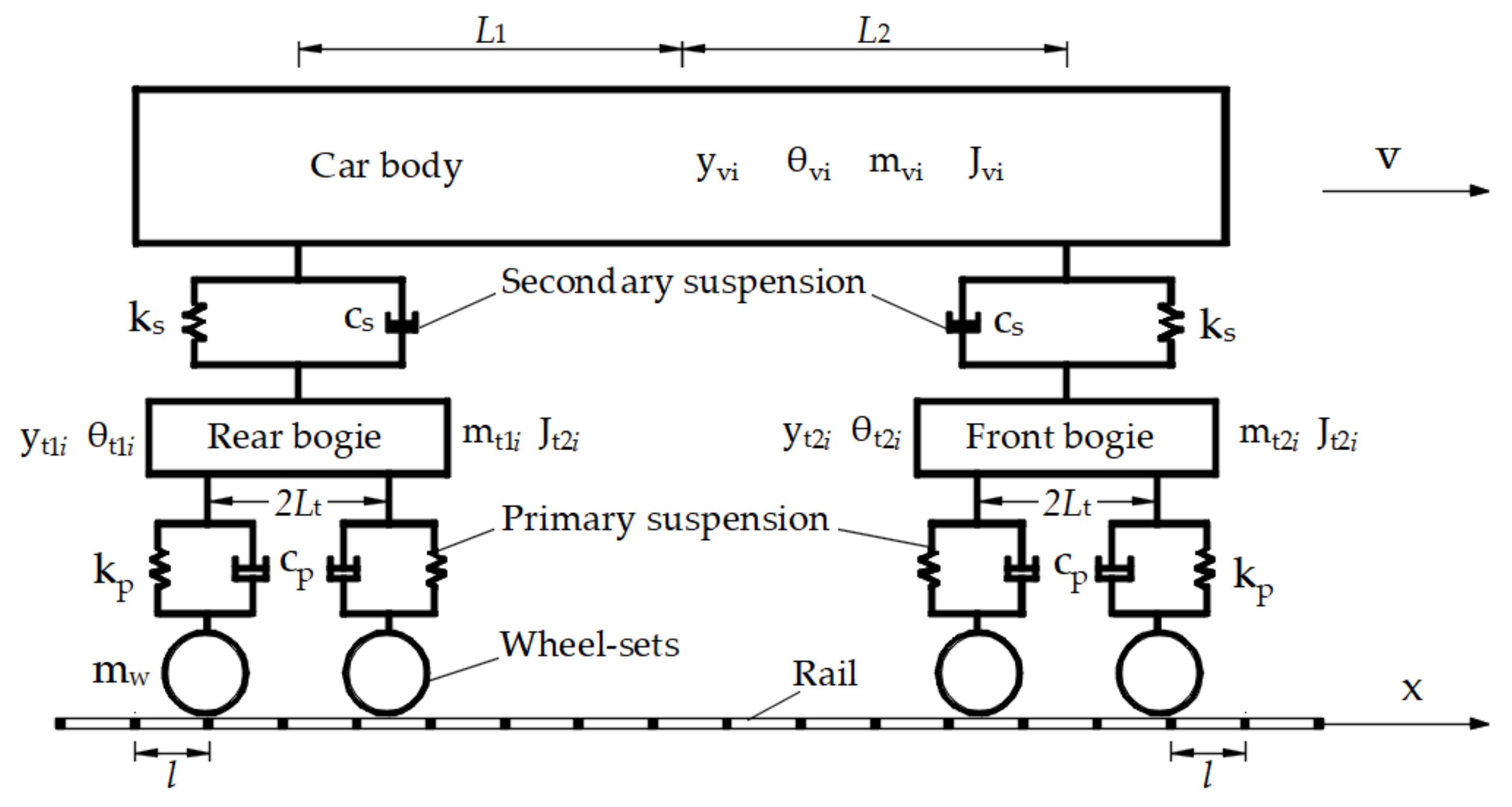
2.1. High-Speed Train Model

The train model consists of several locomotives and vehicles. Each locomotive or vehicle is composed of a car-body, bogie, wheel-sets, and the spring and damping connection between the three components. As shown in Figure 1, the locomotive and vehicle adopt a two-system suspension spring and damping model. The degree of freedom involves the vertical displacement and rotation angle of the car-body and bogie, and the vertical displacement of the wheel-sets. A locomotive has 10 degrees of freedom. The primary suspension spring and damping model are used to connect wheel-sets and the bogie, and the secondary suspension spring and damped model are used to connect the bogie and car-body. Thereinto, $L_1$ is the horizontal distance between the center of mass of the car-body and rear wheel-set; $L_2$ is the horizontal distance between the center of mass of the car-body and front wheel-set; $L_t$ is half of the bogie axle base. $m_{\mathrm{v}i}$, $m_{\mathrm{t}1i}$, and $m_{\mathrm{t}2i}$ respectively, represent the mass of the car body and two bogies of the i-th train. $l$ is the length of the rail element. $J_{\mathrm{v}i}$, $J_{\mathrm{t}1i}$, and $J_{\mathrm{t}2i}$ respectively, represent the rotational inertia of the car body and two bogies of the i-th train. ${\mathrm{y}}_{\mathrm{v}i}$, ${\mathrm{y}}_{\mathrm{t}1i}$, and ${\mathrm{y}}_{\mathrm{t}2i}$ respectively, represent the vertical displacement of the car-body and two bogies of the i-th train. ${\theta }_{\mathrm{v}i}$, ${\theta }_{\mathrm{t}1i}$, and ${\theta }_{\mathrm{t}2i}$ respectively, represent the vertical corner of the car-body and two bogies of the i-th train. $k_{\mathrm{s}}$ and $k_{\mathrm{p}}$ represent the stiffness coefficient of the primary and secondary suspension spring, respectively. $c_{\mathrm{s}}$ and $c_{\mathrm{p}}$ represent damping coefficient the primary and secondary suspension damping, respectively.

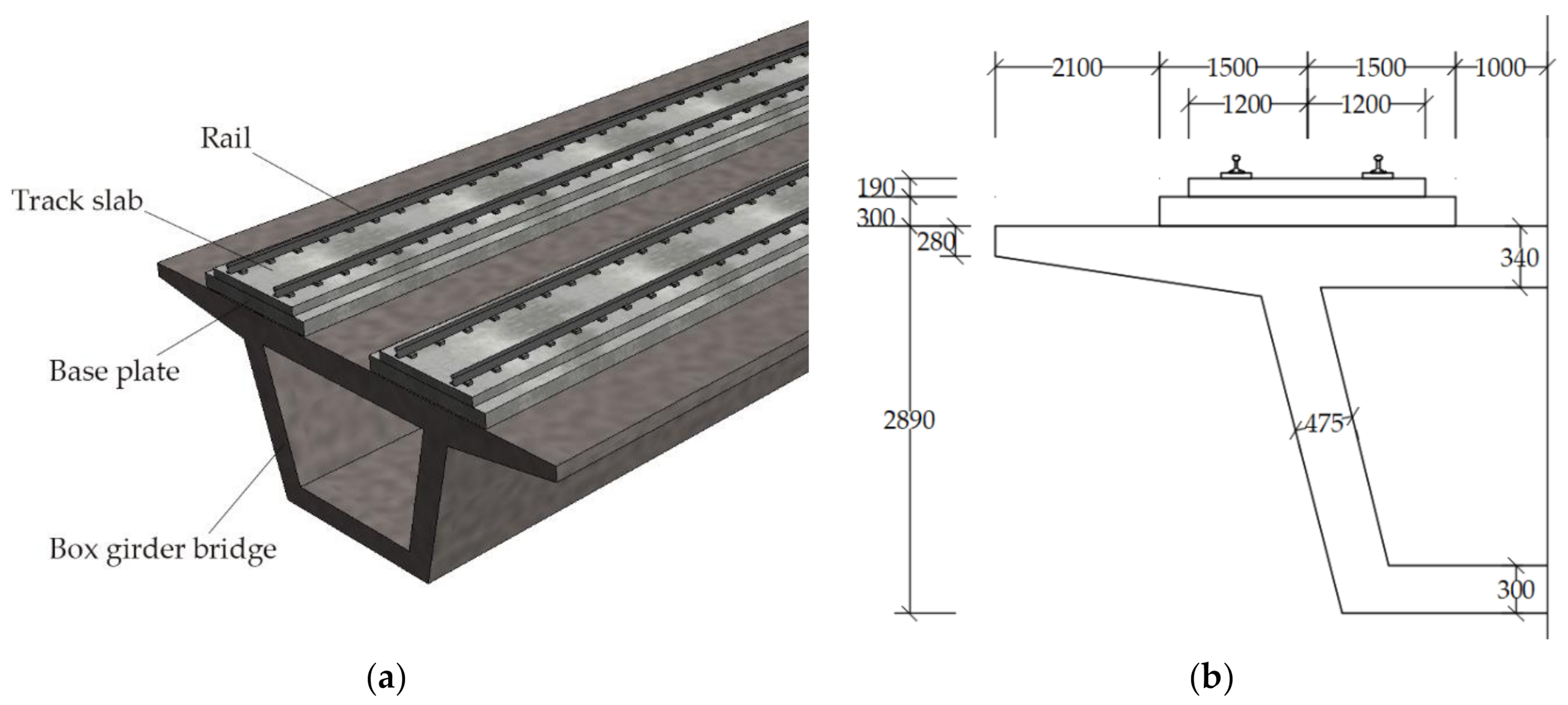
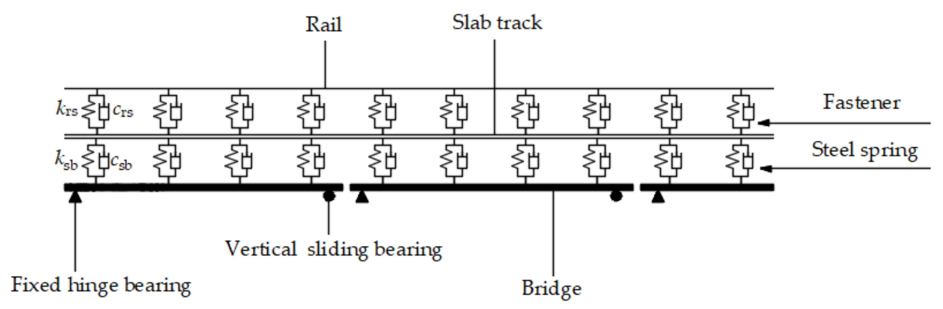
2.2. Dynamic Model of Ballastless Track on Bridge

As shown in Figure 2, the China Railway Track System (CRTS) I type slab track on the bridge is mainly composed of the rail, track slab, base plate and bridge. Thereinto, Figure 2a is schematic diagram of the solid section, and Figure 2b is the section size of one side of the structure of the symmetry axis. The rail is connected to the track slab with the fastener, the track slab is connected to the bridge with the cement asphalt mortar, and the base plate and bridge are connected by an anchoring steel bar.

The mechanical model of the CRTS I type slab track on the bridge is shown in Figure 3. The bridge adopts a simply supported beam model. The section of the bridge is a box girder, as shown in Figure 2a. The left end adopts a fixed hinge bearing to restrain the vertical and the horizontal displacement. The right end adopts a vertical sliding bearing to restrain the vertical displacement. The rail, track slab and bridge are simulated by the beam element in the model, while fasteners and cement asphalt mortar are simulated by linear spring damping. Compared with the bridge, the mass and the flexural rigidity of the base plate are very small; moreover, the base plate and the bridge are tightly connected by an anchoring steel bar, so the base plate and the bridge are regarded as a whole, and the base plate is no longer simulated separately. Thereinto, $k_{\mathrm{rs}}$ and $c_{\mathrm{rs}}$ represent the stiffness and damping coefficients between the rail and track slab. $k_{\mathrm{sb}}$ and $c_{\mathrm{sb}}$ represent the stiffness and damping coefficients between the track slab and the bridge.

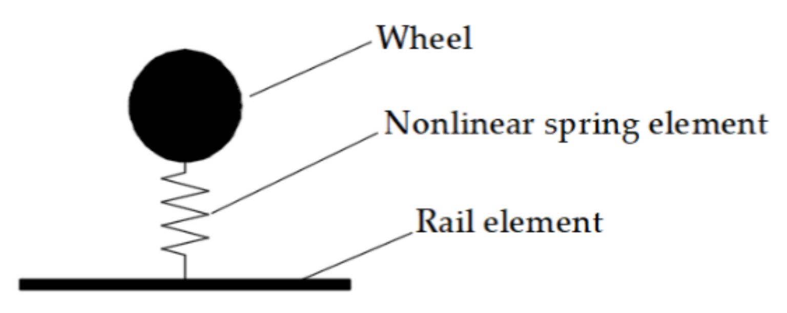
2.3. Wheel-Rail Interaction Relationship

In the vertical plane, the key to interaction between the vehicle submodel and track-bridge submodel is the contact mode between wheel-sets and the track surface. As shown in Figure 4, the contact point between wheel-sets and the rail is modeled by a moving spring. The wheel-rail interaction relationship is simulated by a non-linear spring element. The vertical force between wheel-sets and the rail is determined according to the Hertz non-linear contact theory [26].

Considering the displacement irregularity between the wheel and the rail, the equation of wheel-rail force is as follows:

$$P_j(t)=\left\{\begin{array}{l}\frac{1}{\mathrm{G}}{[Z_{wj}(t)-Z_r({\mathrm{x}}_{pj},t)-Z_0(t)]}^{3/2}\\ 0\end{array}\right.\begin{array}{c}{Z}_{wj}(t)-Z_r({\mathrm{x}}_{pj},t)-Z_0(t)>0\\ Z_{wj}(t)-Z_r({\mathrm{x}}_{pj},t)-Z_0(t)\le 0\end{array},$$

(1)

where, $P_j(t)$ is vertical force between wheel and rail; $\mathrm{G}$ is the wheel-rail contact constant; $Z_{wj}(t)$ is displacement of the j-th wheel at time t; $Z_r({\mathrm{x}}_{pj},t)$ is rail displacement under the j-th wheel at time t; $Z_0(t)$ is track irregularity under the j-th wheel at time t.

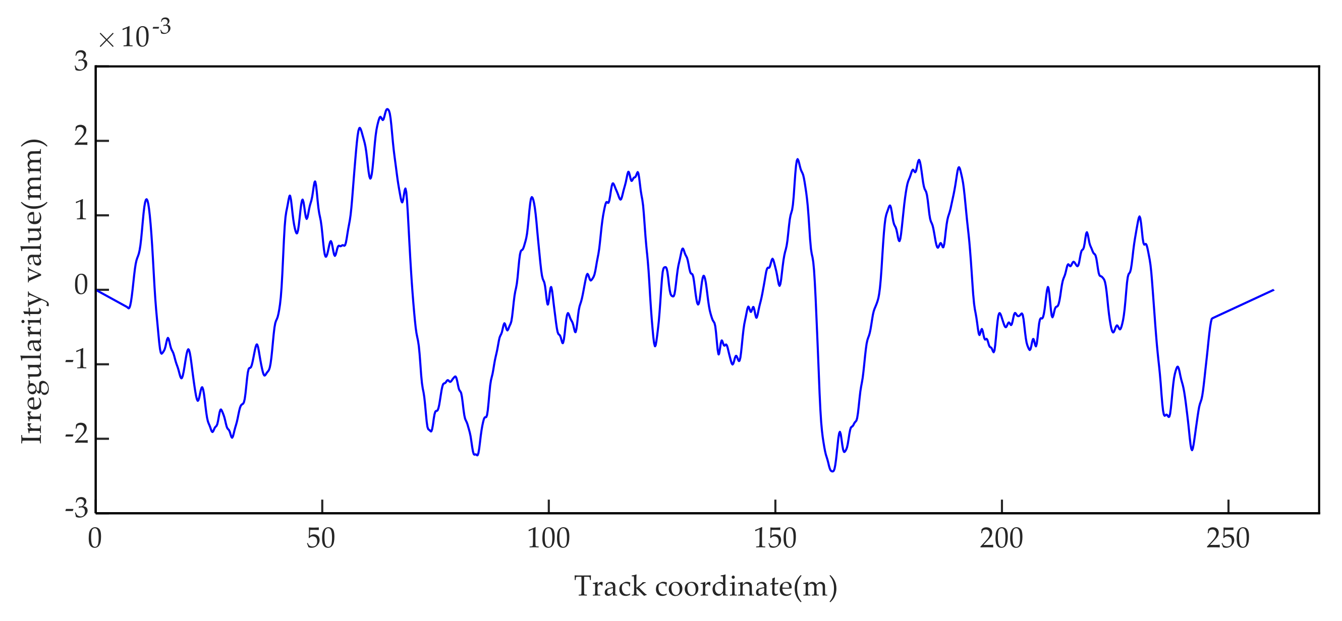
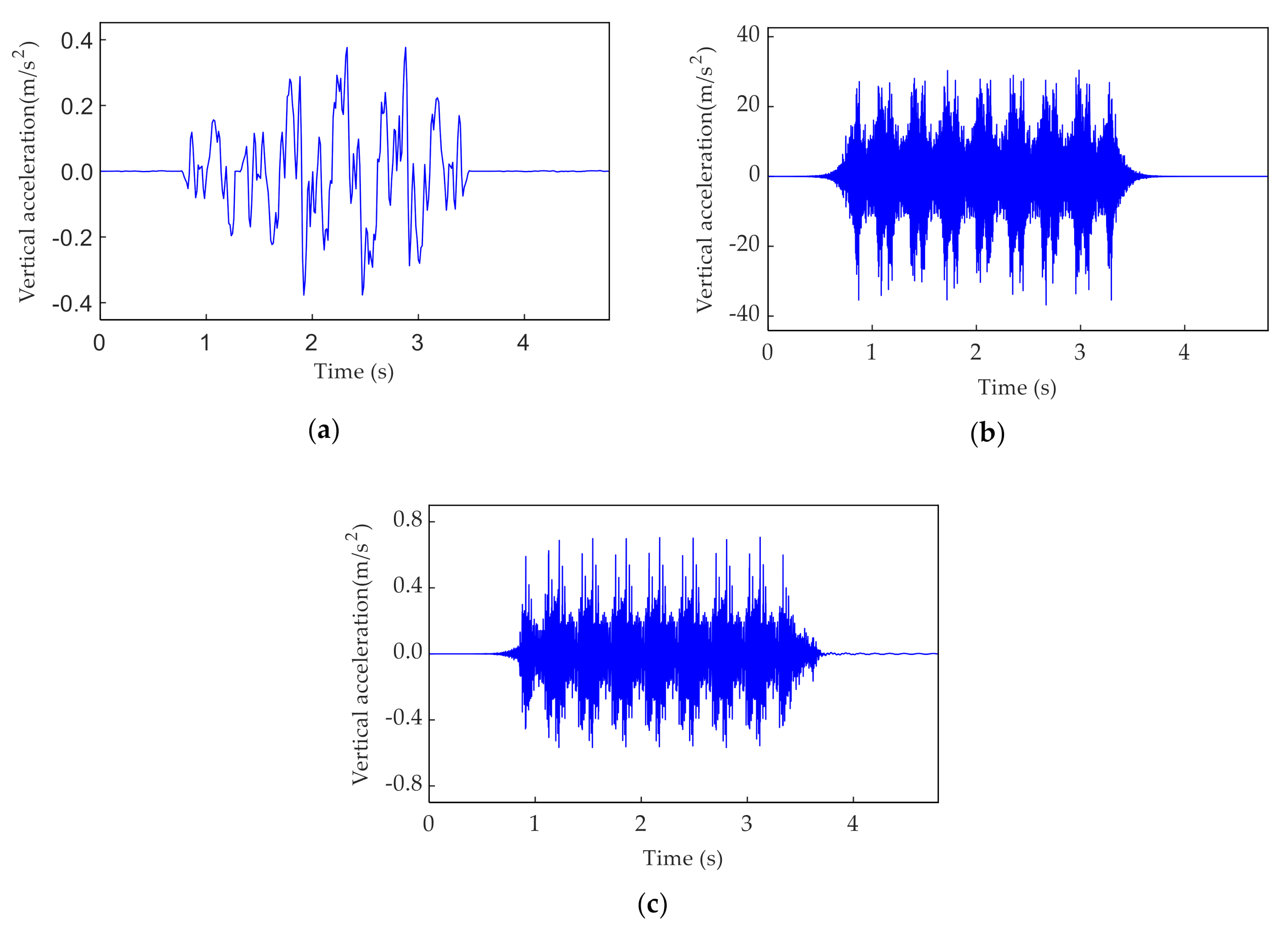
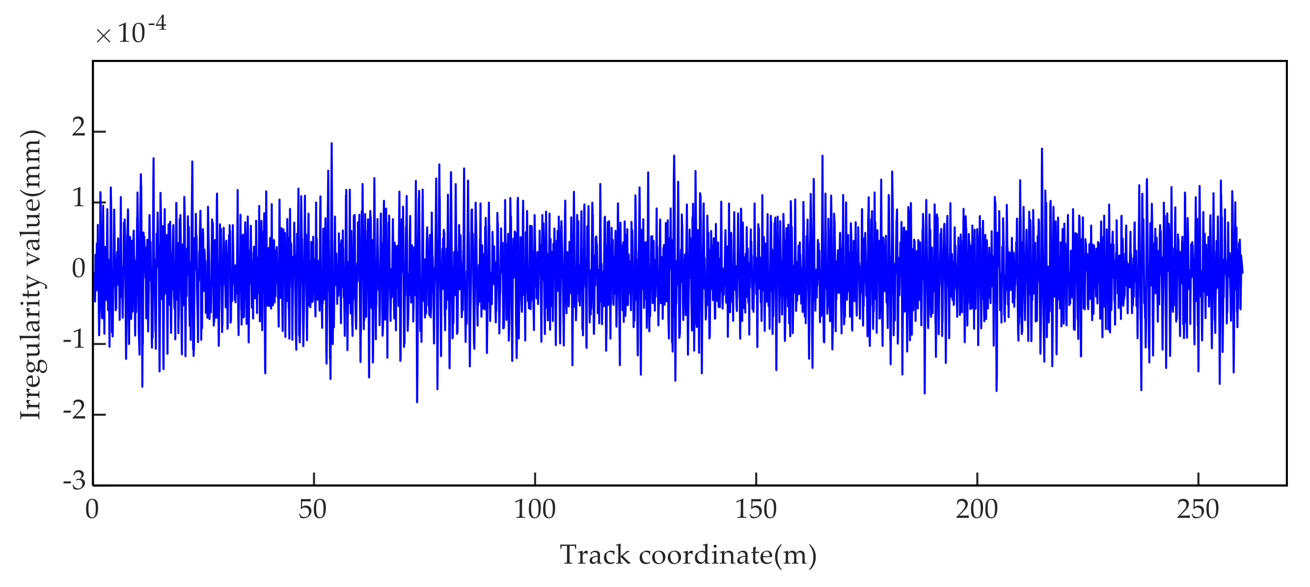
2.4. Track Irregularity Model

Track irregularity taken in this paper is the random irregularity. Its components are very complex and contain various wavelengths. Generally, power spectral density is used to describe the statistical characteristics of track irregularity. In this paper, medium-long wave and short wave are used to fit the track surface to random irregularity.

The simulation of medium-long wave random irregularity is carried out by using the low interference power spectral density of German high-speed railway [27]. The irregular power spectrum of medium-long wave random irregularity is as follows:

$$S(\mathsf{\Omega })=\frac{A_v{\mathsf{\Omega }}_c^2}{({\mathsf{\Omega }}^2+{\mathsf{\Omega }}_r^2)({\mathsf{\Omega }}^2+{\mathsf{\Omega }}_c^2)},$$

(2)

In the formula: $S(\mathsf{\Omega })$ is the power spectral density; $\mathsf{\Omega }$ is the spatial frequency (rad/m); $A_v$ is the roughness constant, its value is 4.032 × 10⁻⁷ m·rad; ${\mathsf{\Omega }}_c$ is the truncation frequency, its value is 0.8246 rad/m; ${\mathsf{\Omega }}_r$ is the truncation frequency, its value is 0.0206 rad/m. The sample of the medium-long wave random irregularity along the track is shown in Figure 5.

According to the research results of Sato [28], the short wave random irregularity has a great influence on the dynamic characteristics of the track. Short wave random irregularity uses the Sato spectrum, and its irregular power spectrum equation is:

$$S\left(\mathsf{\Omega }\right)=\frac{A}{{\mathsf{\Omega }}^3},$$

(3)

where $S(\mathsf{\Omega })$ is the power spectral density; $\mathsf{\Omega }$ is the spatial frequency (rad/m); $A$ is roughness constant and its value is 4.15 × 10⁻⁸ m·rad-5.0 × 10⁻⁷ m·rad. The amplitude and random phase of the spectrum are obtained according to the track random irregularity spectrum, and then a sample of the short wave random irregularity along the track is shown in Figure 6.

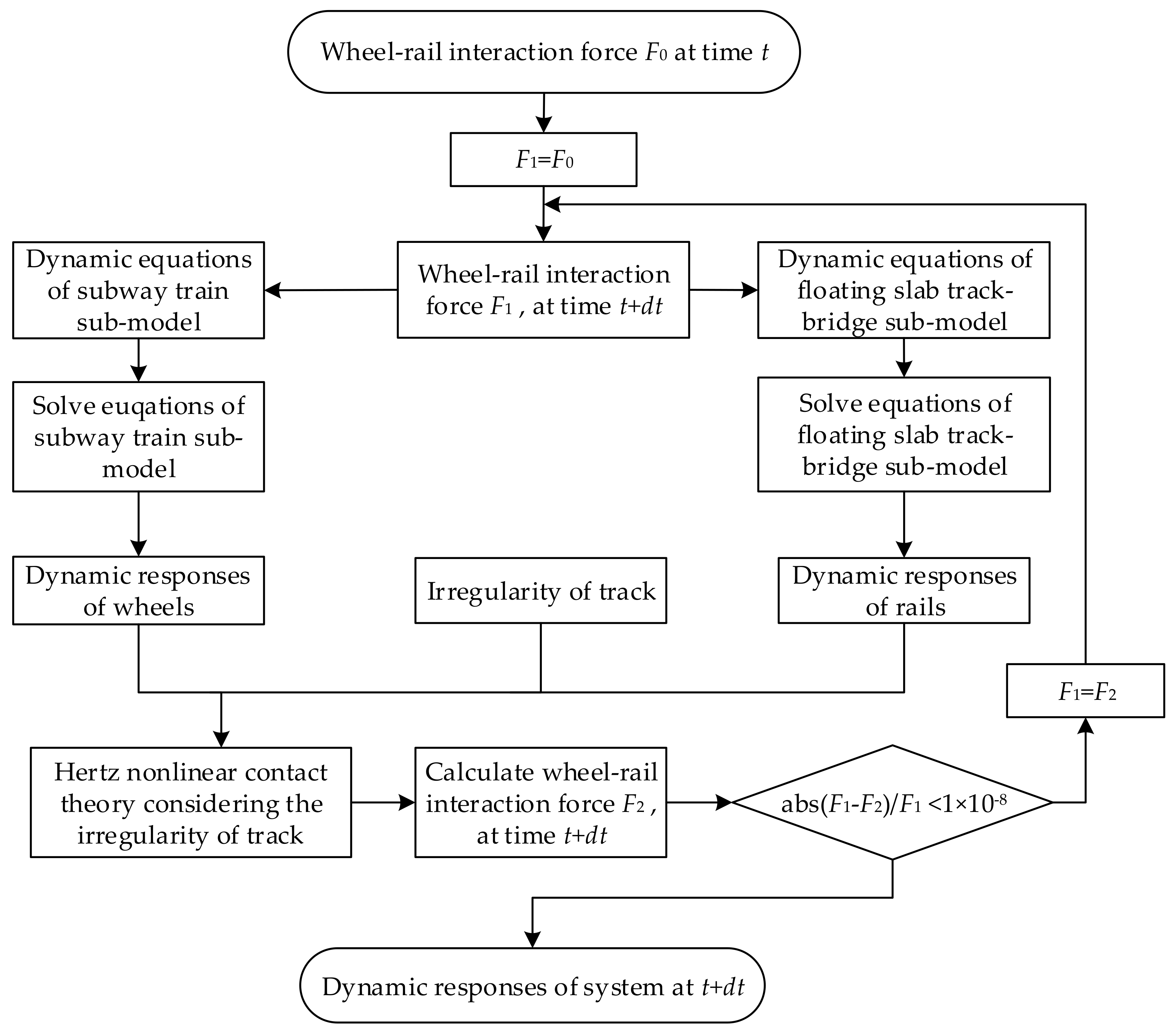
3. Calculation Process

3.1. System Equation

The total potential energy of vehicle subsystem and track-bridge subsystem include inertial potential energy and gravitational potential energy, as well as the elastic strain energy and damping force potential energy between layers of different components. The wheel-rail contact model is the link between the vehicle subsystem and the track-bridge subsystem. According to the principle of stationary value of the total potential energy of elastic system dynamics [29], the vertical coupled vibration equation of the VTB coupled system can be established by using the “set-in-right-position” rule [30], as shown in the following equation:

$$\left[\begin{array}{cccc}{\mathrm{M}}_{\mathrm{v}}& 0& 0& 0\\ 0& {\mathrm{M}}_{\mathrm{r}}& 0& 0\\ 0& 0& {\mathrm{M}}_{\mathrm{s}}& 0\\ 0& 0& 0& {\mathrm{M}}_{\mathrm{b}}\end{array}\right]\left\{\begin{array}{l}{\ddot{\mathrm{X}}}_{\mathrm{v}}\\ {\ddot{\mathrm{X}}}_{\mathrm{r}}\\ {\ddot{\mathrm{X}}}_{\mathrm{s}}\\ {\ddot{\mathrm{X}}}_{\mathrm{b}}\end{array}\right\}+\left[\begin{array}{cccc}{\mathrm{C}}_{\mathrm{v}}& 0& 0& 0\\ 0& {\mathrm{C}}_{\mathrm{r}}& 0& 0\\ 0& 0& {\mathrm{C}}_{\mathrm{s}}& 0\\ 0& 0& 0& {\mathrm{C}}_{\mathrm{b}}\end{array}\right]\left\{\begin{array}{l}{\dot{\mathrm{X}}}_{\mathrm{v}}\\ {\dot{\mathrm{X}}}_{\mathrm{r}}\\ {\dot{\mathrm{X}}}_{\mathrm{s}}\\ {\dot{\mathrm{X}}}_{\mathrm{b}}\end{array}\right\}+\left[\begin{array}{cccc}{\mathrm{K}}_{\mathrm{v}}& 0& 0& 0\\ 0& {\mathrm{K}}_{\mathrm{r}}& 0& 0\\ 0& 0& {\mathrm{K}}_{\mathrm{s}}& 0\\ 0& 0& 0& {\mathrm{K}}_{\mathrm{b}}\end{array}\right]\left\{\begin{array}{l}{\mathrm{X}}_{\mathrm{v}}\\ {\mathrm{X}}_{\mathrm{r}}\\ {\mathrm{X}}_{\mathrm{s}}\\ {\mathrm{X}}_{\mathrm{b}}\end{array}\right\}=\left\{\begin{array}{l}{\mathrm{F}}_{\mathrm{v}}\\ {\mathrm{F}}_{\mathrm{r}}\\ {\mathrm{F}}_{\mathrm{s}}\\ {\mathrm{F}}_{\mathrm{b}}\end{array}\right\},$$

(4)

where, ${\mathrm{X}}_{\mathrm{v}}$, ${\mathrm{X}}_{\mathrm{r}}$, ${\mathrm{X}}_{\mathrm{s}}$, and ${\mathrm{X}}_{\mathrm{b}}$ represent the displacement vectors of the vehicle system, rail, track slab and bridge, respectively; ${\dot{\mathrm{X}}}_{\mathrm{v}}$, ${\dot{\mathrm{X}}}_{\mathrm{r}}$, ${\dot{\mathrm{X}}}_{\mathrm{s}}$, and ${\dot{\mathrm{X}}}_{\mathrm{b}}$ represent the velocity vectors of the vehicle system, rail, track slab and bridge, respectively; ${\ddot{\mathrm{X}}}_{\mathrm{v}}$, ${\ddot{\mathrm{X}}}_{\mathrm{r}}$, ${\ddot{\mathrm{X}}}_{\mathrm{s}}$, and ${\ddot{\mathrm{X}}}_{\mathrm{b}}$ represent the acceleration vectors of the vehicle system, rail, track slab and bridge, respectively; ${\mathrm{M}}_{\mathrm{v}}$, ${\mathrm{M}}_{\mathrm{r}}$, ${\mathrm{M}}_{\mathrm{s}}$, and ${\mathrm{M}}_{\mathrm{b}}$ represent the mass matrix of the vehicle system, rail, track slab and bridge, respectively; ${\mathrm{K}}_{\mathrm{v}}$, ${\mathrm{K}}_{\mathrm{r}}$, ${\mathrm{K}}_{\mathrm{s}}$, and ${\mathrm{K}}_{\mathrm{b}}$ represent the stiffness matrix of the vehicle system, rail, track slab, and bridge, respectively; ${\mathrm{C}}_{\mathrm{v}}$, ${\mathrm{C}}_{\mathrm{r}}$, ${\mathrm{C}}_{\mathrm{s}}$, and ${\mathrm{C}}_{\mathrm{b}}$ represent the damping matrix of the vehicle system, rail, track slab and bridge, respectively; ${\mathrm{F}}_{\mathrm{v}}$, ${\mathrm{F}}_{\mathrm{r}}$, ${\mathrm{F}}_{\mathrm{s}}$, and ${\mathrm{F}}_{\mathrm{b}}$ represent the load vectors of the vehicle system, rail, track slab and bridge, respectively.

Based on the establishment method of the vehicle-track-bridge coupling dynamic equation [31], the matrix expression in the equation is as follows:

3.1.1. Equation of the Vehicle System

The vehicle displacement vector ${\mathrm{X}}_{\mathrm{v}}$ is expressed as:

$${\mathrm{X}}_{\mathrm{v}}={[{\mathrm{X}}_{\mathrm{v}1}\hspace{1em}{\mathrm{X}}_{\mathrm{v}2}\hspace{1em}\cdots \hspace{1em}{\mathrm{X}}_{\mathrm{v}{n}_{\mathrm{v}}}]}^{\mathrm{T}},$$

(5)

$${\mathrm{X}}_{\mathrm{v}i}=[y_{\mathrm{v}i}\hspace{1em}{\theta }_{\mathrm{v}i}\hspace{1em}{y}_{\mathrm{t}1i}\hspace{1em}{\theta }_{\mathrm{t}1i}\hspace{1em}{y}_{\mathrm{t}2i}\hspace{1em}{\theta }_{\mathrm{t}2i}],$$

(6)

where, $n_{\mathrm{v}}$ represents the total number of the vehicles; ${\mathrm{X}}_{\mathrm{v}i}$ represents the displacement vector of the i-th vehicle. ${\mathrm{y}}_{\mathrm{v}i}$, ${\mathrm{y}}_{\mathrm{t}1i}$, and ${\mathrm{y}}_{\mathrm{t}2i}$ respectively represent the vertical displacement of the car body and two bogies of the i-th train. ${\theta }_{\mathrm{v}i}$, ${\theta }_{\mathrm{t}1i}$, and ${\theta }_{\mathrm{t}2i}$ respectively, represent the vertical corner of the car body and two bogies of the i-th train. The schematic diagram of parameters can be referred to in Figure 1.

The vehicle mass matrix ${\mathrm{M}}_{\mathrm{v}}$ is expressed as:

$${\mathrm{M}}_{\mathrm{v}}=\mathrm{diag}[{\mathrm{M}}_{\mathrm{v}1}\hspace{1em}{\mathrm{M}}_{\mathrm{v}2}\hspace{1em}\cdots \hspace{1em}{\mathrm{M}}_{\mathrm{v}{n}_{\mathrm{v}}}],$$

(7)

$${\mathrm{M}}_{\mathrm{v}i}=\mathrm{diag}[m_{\mathrm{v}i}\hspace{1em}{J}_{\mathrm{v}i}\hspace{1em}{m}_{\mathrm{t}1i}\hspace{1em}{J}_{\mathrm{t}1i}\hspace{1em}{m}_{\mathrm{t}2i}\hspace{1em}{J}_{\mathrm{t}2i}],$$

(8)

where, ${\mathrm{M}}_{\mathrm{v}i}$ is the mass matrix of the i-th vehicle. $m_{\mathrm{v}i}$, $m_{\mathrm{t}1i}$, and $m_{\mathrm{t}2i}$ respectively, represent the mass of the car body and two bogies of the i-th train. $J_{\mathrm{v}i}$, $J_{\mathrm{t}1i}$, and $J_{\mathrm{t}2i}$ respectively represent the rotational inertia of the car body and two bogies of the i-th train. The schematic diagram of parameters can be referred to in Figure 1.

The vehicle stiffness matrix ${\mathrm{K}}_{\mathrm{v}}$ is expressed as:

$${\mathrm{K}}_{\mathrm{v}}=\mathrm{diag}[{\mathrm{K}}_{\mathrm{v}1}\hspace{1em}{\mathrm{K}}_{\mathrm{v}2}\hspace{1em}\cdots \hspace{1em}{\mathrm{K}}_{\mathrm{v}{n}_{\mathrm{v}}}],$$

(9)

$${\mathrm{K}}_{\mathrm{v}i}= \left[\begin{array}{cccccc}2k_{\mathrm{s}}& -k_{\mathrm{s}}{L}_1+k_{\mathrm{s}}{L}_2& -k_{\mathrm{s}}& 0& -k_{\mathrm{s}}& 0\\ -k_{\mathrm{s}}{L}_1+k_{\mathrm{s}}{L}_2& k_{\mathrm{s}}{L}_1^2+k_{\mathrm{s}}{L}_2^2& k_{\mathrm{s}}{L}_1& 0& -k_{\mathrm{s}}{L}_2& 0\\ -k_{\mathrm{s}}& k_{\mathrm{s}}{L}_1& k_{\mathrm{s}}+2k_{\mathrm{p}}& 0& 0& 0\\ 0& 0& 0& 2k_{\mathrm{p}}{L}_{\mathrm{t}}^2& 0& 0\\ -k_{\mathrm{s}}& -k_{\mathrm{s}}{L}_2& 0& 0& k_{\mathrm{s}}+2k_{\mathrm{p}}& 0\\ 0& 0& 0& 0& 0& 2k_{\mathrm{p}}{L}_{\mathrm{t}}^2\end{array}\right],$$

(10)

where, ${\mathrm{K}}_{\mathrm{v}i}$ is the stiffness matrix of the i-th vehicle; the parameter in the formula can be referred to in Figure 1. In the same way, damping matrix ${\mathrm{C}}_{\mathrm{v}}$ can be obtained from the Formulas (9) and (10) by replacing $k_{\mathrm{s}}$ and $k_{\mathrm{p}}$ in the stiffness matrix with $c_{\mathrm{s}}$ and $c_{\mathrm{p}}$. The schematic diagram of parameters can be referred to in Figure 1.

3.1.2. Equation of the Rail

The rail displacement vector ${\mathrm{X}}_{\mathrm{r}}$ is expressed as:

$${\mathrm{X}}_{\mathrm{r}}={[{\mathrm{X}}_{\mathrm{r}1}\hspace{1em}{\mathrm{X}}_{\mathrm{r}2}\hspace{1em}\cdots \hspace{1em}{\mathrm{X}}_{\mathrm{r}{n}_{\mathrm{r}}}]}^{\mathrm{T}},$$

(11)

where, $n_{\mathrm{r}}$ is the total number of degrees of freedom; ${\mathrm{X}}_{\mathrm{r}i}$ represents the displacement vector of the i-th rail element.

The rail mass matrix ${\mathrm{M}}_{\mathrm{r}}$ is expressed as:

$${\mathrm{M}}_{\mathrm{r}}{= \mathrm{M}}_{\mathrm{r}1}{+ \mathrm{M}}_{\mathrm{r}2},$$

(12)

$${\mathrm{N}}_{\mathrm{r}}= [0\hspace{1em}0\hspace{1em}\cdots \hspace{1em}0\hspace{1em}{N}_1\hspace{1em}{N}_2\hspace{1em}{N}_3\hspace{1em}{N}_4\hspace{1em}0\hspace{1em}\cdots \hspace{1em}0\hspace{1em}0\hspace{1em}],$$

(13)

$${\mathrm{N}}_{ji}= [0\hspace{1em}0\hspace{1em}\cdots \hspace{1em}0\hspace{1em}{N}_1\hspace{1em}{N}_2\hspace{1em}{N}_3\hspace{1em}{N}_4\hspace{1em}0\hspace{1em}\cdots {\hspace{1em}0\hspace{1em}0\hspace{1em}]}_{\xi ={\xi }_{ji}},$$

(14)

$$\begin{array}{ll}{\mathrm{N}}_1= 1 - 3(\xi /l{)}^2 + 2(\xi /l{)}^3& { \mathrm{N}}_1= \xi [1 - 2(\xi /l) + (\xi /l{)}^2]\\ {\mathrm{N}}_3= 3(\xi /l{)}^2 - 2(\xi /l{)}^3& { \mathrm{N}}_4= 3\left[\right(\xi /l{)}^2 - (\xi /l)]\end{array},$$

(15)

$${\mathrm{M}}_{\mathrm{r}2}={\displaystyle \sum _{i=1}^{N_{\mathrm{v}}}{\displaystyle \sum _{j=1}^4{m}_{\mathrm{w}}·{\mathrm{N}}_{ji}^{\mathrm{T}}}}·{\mathrm{N}}_{ji},$$

(16)

where ${\mathrm{M}}_{\mathrm{r}1}$ (with order $n_{\mathrm{r}}\times n_{\mathrm{r}}$) is the mass matrix of the rail itself, which can be obtained by integrating all the rail element matrices ${\displaystyle \underset{0}{\overset{l}{\int }}{\overline{m}}_{\mathrm{r}}{\mathrm{N}}_{\mathrm{r}}^{\mathrm{T}}{\mathrm{N}}_{\mathrm{r}}d\xi }$. ${\mathrm{N}}_{\mathrm{r}}$ is the shape function matrix of the rail itself, and ${\overline{m}}_{\mathrm{r}}$ is the mass per unit length of rail. ${\mathrm{M}}_{\mathrm{r}2}$ is the mass matrix of the rail caused by all wheel-sets. ${\mathrm{N}}_{ji}$ is the shape function matrix of the rail unit where the j-th wheel-sets of the i-th vehicle are located. ${\xi }_{ji}$ is the distance between the j-th wheel-sets of the i-th vehicle and the left node of the rail element in contact with wheel-sets.

The rail stiffness matrix ${\mathrm{K}}_{\mathrm{r}}$ is expressed as:

$${\mathrm{K}}_{\mathrm{r}}{= \mathrm{K}}_{\mathrm{r}1}{+ \mathrm{K}}_{\mathrm{r}2}+{ \mathrm{K}}_{\mathrm{r}3},$$

(17)

$${\mathrm{K}}_{\mathrm{r}2}={\displaystyle \sum _{i=1}^{N_{\mathrm{v}}}{\displaystyle \sum _{j=1}^4[k_{\mathrm{v}}·{\mathrm{N}}_{ji}^{\mathrm{T}}}}·{\mathrm{N}}_{ji}+{ (\mathrm{c}}_{\mathrm{v}}v+m_{\mathrm{w}}a){\mathrm{N}}_{ji}^{\mathrm{T}}·{\mathrm{N}}_{ji}^{\prime }+m_{\mathrm{w}}{v}^2{\mathrm{N}}_{ji}^{\mathrm{T}}·{\mathrm{N}}_{ji}^{″}],$$

(18)

$${\mathrm{N}}_{\mathrm{s}i}= [0\hspace{1em}0\hspace{1em}\cdots \hspace{1em}0\hspace{1em}{N}_1\hspace{1em}{N}_2\hspace{1em}{N}_3\hspace{1em}{N}_4\hspace{1em}0\hspace{1em}\cdots \hspace{1em}0\hspace{1em}0],$$

(19)

where ${\mathrm{K}}_{\mathrm{r}1}$ is the stiffness matrix of the rail itself, which can be obtained by integrating all rail element matrices ${\displaystyle \underset{0}{\overset{l}{\int }}{E}_{\mathrm{r}}{I}_{\mathrm{r}}{\mathrm{N}}_{\mathrm{r}}^{″\mathrm{T}}{\mathrm{N}}_{\mathrm{r}}^{″}d\xi }$. $E_{\mathrm{r}}$ is the Young’s modulus of the rail, $I_{\mathrm{r}}$ is the moment of inertia of the rail section. ${\mathrm{K}}_{\mathrm{r}2}$ is the stiffness matrix of the rail caused by vehicles. ${\mathrm{N}}_{\mathrm{s}i}$ is the shape function matrix of the i-th track slab, and $k_{\mathrm{rs}}$ is the stiffness coefficient between the rail and the track slab. ${\mathrm{K}}_{\mathrm{r}3}$ is stiffness matrix of the rail caused by track slabs, which can be obtained by ${\displaystyle \underset{0}{\overset{l}{\int }}{k}_{\mathrm{rs}}{\mathrm{N}}_{\mathrm{s}i}^{\mathrm{T}}{\mathrm{N}}_{\mathrm{s}i}d\xi }$.

The rail damping matrix ${\mathrm{C}}_{\mathrm{r}}$ is expressed as:

$${\mathrm{C}}_{\mathrm{r}}{= \mathrm{C}}_{\mathrm{r}1}{+ \mathrm{C}}_{\mathrm{r}2},$$

(20)

$${\mathrm{C}}_{\mathrm{r}1}={\displaystyle \sum _{i=1}^{N_{\mathrm{r}}}{\displaystyle \sum _{j=1}^4(c_{\mathrm{w}}·{\mathrm{N}}_{ji}^{\mathrm{T}}}}·{\mathrm{N}}_{ji}+ 2m_{\mathrm{w}}v·{\mathrm{N}}_{ji}^{\mathrm{T}}{\mathrm{N}}_{ji}),$$

(21)

where ${\mathrm{C}}_{\mathrm{r}1}$ is the damping matrix of the rail caused by vehicles; ${\mathrm{C}}_{\mathrm{r}2}$ is the damping matrix of the rail between the rail and the track slab, which can be obtained by ${\displaystyle \underset{0}{\overset{l}{\int }}{c}_{\mathrm{rs}}{\mathrm{N}}_{\mathrm{s}i}^{\mathrm{T}}{\mathrm{N}}_{\mathrm{s}i}d\xi }$. $c_{\mathrm{rs}}$ is the damping coefficient between the rail and the track slab.

3.1.3. Equation of the Track Slab

The track slab displacement vector ${\mathrm{X}}_{\mathrm{s}}$ is expressed as:

$${\mathrm{X}}_{\mathrm{s}}=[{\mathrm{X}}_{\mathrm{s}1}\hspace{1em}{\mathrm{X}}_{\mathrm{s}2}\hspace{1em}\cdots \hspace{1em}{\mathrm{X}}_{\mathrm{s}{n}_{\mathrm{s}}}{]}^{\mathrm{T}},$$

(22)

where, $n_{\mathrm{s}}$ represent the total number of track slabs, ${\mathrm{X}}_{\mathrm{s}i}$ represents the displacement vector of the i-th track slab.

The track slab mass matrix ${\mathrm{M}}_{\mathrm{s}}$ is expressed as:

$${\mathrm{M}}_{\mathrm{s}}= \mathrm{diag}[{\mathrm{M}}_{\mathrm{s}1}\hspace{1em}{\mathrm{M}}_{\mathrm{s}2}\hspace{1em}\cdots \hspace{1em}{\mathrm{M}}_{\mathrm{s}{n}_{\mathrm{s}}}],$$

(23)

where ${\mathrm{M}}_{\mathrm{s}i}$ is the mass matrix of the i-th track slab, which can be obtained by integrating all element matrices ${\displaystyle \underset{0}{\overset{l}{\int }}{\overline{m}}_{\mathrm{s}}{\mathrm{N}}_{\mathrm{s}i}^{\mathrm{T}}{\mathrm{N}}_{\mathrm{s}i}d\xi }$. ${\overline{m}}_{\mathrm{s}}$ is the mass of the track slab per unit length, and ${\mathrm{N}}_{\mathrm{s}i}$ is the shape function matrix of the i-th track slab.

The track slab stiffness matrix ${\mathrm{K}}_{\mathrm{s}}$ is expressed as:

$${\mathrm{K}}_{\mathrm{s}}= \mathrm{diag}[{\mathrm{K}}_{\mathrm{s}1}\hspace{1em}{\mathrm{K}}_{\mathrm{s}2}\hspace{1em}\cdots \hspace{1em}{\mathrm{K}}_{\mathrm{s}{n}_{\mathrm{s}}}],$$

(24)

$${\mathrm{K}}_{\mathrm{s}i}= {\mathrm{K}}_{\mathrm{s}i1}+ {\mathrm{K}}_{\mathrm{s}i2}+ {\mathrm{K}}_{\mathrm{s}i3},$$

(25)

where ${\mathrm{K}}_{\mathrm{s}i}$ is the stiffness matrix of the i-th track slab. ${\mathrm{K}}_{\mathrm{s}i1}$, ${\mathrm{K}}_{\mathrm{s}i2}$, and ${\mathrm{K}}_{\mathrm{s}i3}$ respectively, are the stiffness matrix of the i-th track slab by itself, the rail and the bridge, and they can be obtained by integrating element matrices ${\displaystyle \underset{0}{\overset{l}{\int }}{E}_{\mathrm{s}}{I}_{\mathrm{s}}{\mathrm{N}}_{\mathrm{s}i}^{″\mathrm{T}}{\mathrm{N}}_{\mathrm{s}i}^{″}d\xi }$, $k_{\mathrm{rs}}{\mathrm{N}}_{\mathrm{s}i}^{\mathrm{T}}{\mathrm{N}}_{\mathrm{s}i}$ and ${\displaystyle \underset{0}{\overset{l}{\int }}{\overline{k}}_{\mathrm{sb}}{\mathrm{N}}_{\mathrm{b}i}^{\mathrm{T}}{\mathrm{N}}_{\mathrm{b}i}d\xi }$ respectively. $E_{\mathrm{s}}$ is the Young’s modulus of the rail, $I_{\mathrm{s}}$ is the moment of inertia of the rail section. ${\overline{k}}_{\mathrm{sb}}$ is the stiffness coefficient between the track slab and the bridge. ${\mathrm{N}}_{\mathrm{b}i}$ is the shape function matrix of the i-th multi-span bridge and is the same as ${\mathrm{N}}_{\mathrm{s}i}$.

The track slab damping matrix ${\mathrm{C}}_{\mathrm{s}}$ is expressed as:

$${\mathrm{C}}_{\mathrm{s}}=\mathrm{diag}[{\mathrm{C}}_{\mathrm{s}1}\hspace{1em}{\mathrm{C}}_{\mathrm{s}2}\hspace{1em}\cdots \hspace{1em}{\mathrm{C}}_{\mathrm{s}{n}_{\mathrm{s}}}],$$

(26)

$${\mathrm{C}}_{\mathrm{s}i}={\mathrm{C}}_{\mathrm{s}i1}+ {\mathrm{C}}_{\mathrm{s}i2},$$

(27)

Thereinto, ${\mathrm{C}}_{\mathrm{s}i1}$ and ${\mathrm{C}}_{\mathrm{s}i2}$ respectively, are the damping matrix of the i-th track slab by the rail and the bridge, and they can be obtained by integrating element matrices $c_{\mathrm{rs}}{\mathrm{N}}_{\mathrm{s}i}^{\mathrm{T}}{\mathrm{N}}_{\mathrm{s}i}$ and ${\displaystyle \underset{0}{\overset{l}{\int }}{\overline{c}}_{\mathrm{sb}}{\mathrm{N}}_{\mathrm{s}i}^{\mathrm{T}}{\mathrm{N}}_{\mathrm{s}i}d\xi }$ respectively. ${\overline{c}}_{\mathrm{sb}}$ is the damping coefficient between the track slab and the bridge.

3.1.4. Equation of the Bridge

The bridge displacement vector ${\mathrm{X}}_{\mathrm{b}}$ is expressed as:

$${\mathrm{X}}_{\mathrm{b}}=[{\mathrm{X}}_{\mathrm{b}1}\hspace{1em}{\mathrm{X}}_{\mathrm{b}2}\hspace{1em}\cdots \hspace{1em}{\mathrm{X}}_{\mathrm{b}{n}_{\mathrm{b}}}{]}^{\mathrm{T}},$$

(28)

where $n_{\mathrm{b}}$ represents the total number of multi-span bridges; ${\mathrm{X}}_{\mathrm{b}i}$ represents the displacement vector of the i-th multi-span bridges.

The bridge mass matrix ${\mathrm{M}}_{\mathrm{b}}$ is expressed as:

$${\mathrm{M}}_{\mathrm{b}}= \mathrm{diag}[{\mathrm{M}}_{\mathrm{b}1}\hspace{1em}{\mathrm{M}}_{\mathrm{b}2}\hspace{1em}\cdots \hspace{1em}{\mathrm{M}}_{\mathrm{b}{n}_{\mathrm{b}}}],$$

(29)

where ${\mathrm{M}}_{\mathrm{b}i}$ is the mass matrix of the i-th multi-span bridge, which can be obtained by integrating all element mass matrices ${\displaystyle \underset{0}{\overset{l}{\int }}{\overline{m}}_{\mathrm{b}}{\mathrm{N}}_{\mathrm{b}i}^{\mathrm{T}}\mathrm{N}d\xi }$. ${\overline{m}}_{\mathrm{b}}$ is the mass of the bridge per unit length, and ${\mathrm{N}}_{\mathrm{b}i}$ is the shape function matrix of the i-th multi-span bridge and is the same as ${\mathrm{N}}_{\mathrm{s}i}$.

The bridge stiffness matrix ${\mathrm{K}}_{\mathrm{b}}$ is expressed as:

$${\mathrm{K}}_{\mathrm{b}}{=\mathrm{K}}_{\mathrm{b}1}{+ \mathrm{K}}_{\mathrm{b}2},$$

(30)

where ${\mathrm{K}}_{\mathrm{b}1}$ is the stiffness matrix of the bridge itself, which can be obtained by integrating all bridge element matrices ${\displaystyle \underset{0}{\overset{l}{\int }}{E}_{\mathrm{b}}{I}_{\mathrm{b}}{\mathrm{N}}_{\mathrm{b}i}^{″\mathrm{T}}{\mathrm{N}}^{″}}d\xi$. $E_{\mathrm{b}}$ is the Young’s modulus of the bridge, and $I_{\mathrm{b}}$ is the moment of inertia of the bridge section. ${\mathrm{K}}_{\mathrm{b}2}$ is the stiffness matrix of the bridge caused by the track slab, and it can be obtained by integrating matric ${\displaystyle \underset{0}{\overset{l}{\int }}{\overline{k}}_{\mathrm{sb}}{\mathrm{N}}_{\mathrm{b}i}^{\mathrm{T}}{\mathrm{N}}_{\mathrm{b}i}d\xi }$.

The bridge damping matrix ${\mathrm{C}}_{\mathrm{b}}$ is expressed as:

$${\mathrm{C}}_{\mathrm{b}}{=\mathrm{C}}_{\mathrm{b}1}{+ \mathrm{C}}_{\mathrm{b}2},$$

(31)

$${\mathrm{C}}_{\mathrm{b}1}=\alpha ·{\mathrm{M}}_{\mathrm{b}}+ \beta ·{\mathrm{K}}_{\mathrm{b}1},$$

(32)

where ${\mathrm{C}}_{\mathrm{b}1}$ is the damping matrix of the bridge itself, and can be obtained from the Rayleigh damping. $\alpha$ and $\beta$ are damping coefficients [32]. ${\mathrm{C}}_{\mathrm{b}2}$ is the bridge damping matrix caused by the track slab, and it can be obtained by integrating matric ${\displaystyle \underset{0}{\overset{l}{\int }}{\overline{c}}_{\mathrm{sb}}{\mathrm{N}}_{\mathrm{b}i}^{\mathrm{T}}{\mathrm{N}}_{\mathrm{b}i}d\xi }$.

The non-zero load vector includes the load vector of vehicle ${\mathrm{F}}_{\mathrm{v}}$ and the load vector of rail ${\mathrm{F}}_{\mathrm{r}}$, and the equation can be referred to in the research by Lou [31].

3.2. Calculation Method

The Newmark method [33] is used to solve the vehicle-track-bridge coupled vibration equations. When the numerical integration reaches the time $t_k$, ${\ddot{\mathrm{X}}}_k$, ${\dot{\mathrm{X}}}_k$, and ${\mathrm{X}}_k$ are acceleration, velocity, and displacement, respectively. The balance equation can be expressed as:

$$\mathrm{M}{\ddot{\mathrm{X}}}_k+{\mathrm{C} \dot{\mathrm{X}}}_k+\mathrm{K}({\mathrm{X}}_k)=F(t_k),$$

(33)

The speed and acceleration of the next time ($t_{k+1}=t_k+dt$) can be expressed as:

$${\mathrm{X}}_{k+1}{=\mathrm{X}}_k+dt\dot{\mathrm{X}}+{(dt)}^2(\frac{1}{2}-\beta ){\ddot{\mathrm{X}}}_k+{(dt)}^2\beta {\ddot{\mathrm{X}}}_{k+1},$$

(34)

$${\dot{\mathrm{X}}}_{k+1}={\dot{\mathrm{X}}}_k+dt(\frac{1}{2}-\gamma )\ddot{\mathrm{X}}+dt\gamma {\ddot{\mathrm{X}}}_{k+1},$$

(35)

where, ${\ddot{\mathrm{X}}}_{k+1}$, ${\dot{\mathrm{X}}}_{k+1}$, and ${\mathrm{X}}_{k+1}$ are acceleration, velocity and displacement, respectively, at time $t_{k+1}$. $\beta$ and $\gamma$ are the parameters of the method.

Equations (34) and (35) are substituted into the balance of Equation (33). Then, with ${\mathrm{X}}_{k+1}$ used as the unknown of the algebraic equation, the solution at $t_{k+1}=t_k+dt$ can be obtained after iteration.

When t = 0, the static equation of the system is solved under the action of gravity, and the result of displacement is used as the initial value. According to the static balance Equation (4), the wheel-rail interaction force $F_0$ between the wheel and the rail can be obtained.

When t > 0, the wheel-rail interaction model is used considering track random irregularity. Please refer to Figure 7 for the detailed calculation process. $F_0$ is taken as the initial wheel-rail force, and the displacement, velocity and acceleration of each degree of freedom, as well as the interaction forces between wheels and rails being calculated iteratively.

3.3. System Parameters

The high-speed train uses four vehicles, and the parameters of the vehicle adopt the data of the China Railway High-speed type 3 passenger car. The speed of the train adopts three different speeds, and they are 200, 300 and 400 km/h, respectively. The detailed parameters of the vehicle are shown in

Table 1. The Parameters of the Vehicle Submodel.

Parameter	Notation	Value
Mass of the car body	$m_{\mathrm{v}i}$	19,800 kg
Mass of the wheel-sets	$m_{\mathrm{w}}$	1000 kg
Rotational inertia of the car body	$J_{\mathrm{v}i}$	970,200 kg·m2
Mass of the rear bogie	$m_{\mathrm{t}1i}$	1600 kg
Mass of the front bogie	$m_{\mathrm{t}2i}$	1600 kg
Rotational inertia of the rear bogie	$J_{\mathrm{t}1i}$	876 kg·m2
Rotational inertia of the front bogie	$J_{\mathrm{t}2i}$	876 kg·m2
Vertical damping of the primary suspension	$c_{\mathrm{p}}$	19,600 N·s·m−1
Vertical stiffness of the primary suspension	$k_{\mathrm{p}}$	1,176,000 N·m−1
Vertical damping of the secondary suspension	$c_{\mathrm{s}}$	19,600 N·s·m−1
Vertical stiffness of the secondary suspension	$k_{\mathrm{s}}$	441,000 N·m−1
Half of the bogie axle base	$L_t$	0.625 m
Mass of the wheel-sets	$m_{\mathrm{w}}$	1000 kg
Distance between the center of mass of the Car body and rear wheel-sets	$L_1$	8.75 m
Distance between the center of mass of the Car body and front wheel-sets	$L_2$	8.75 m
Speed of the train	$v$	200, 300 and 400 km/h

. A CRTS I slab ballastless track is adopted in the track structure. The bridge is simply a supported beam bridge. The detailed parameters of the track and bridge are shown in

Table 2. The Parameters of Track-Bridge Submodel.

Parameter	Notation	Value
Elastic modulus of the rail	$E_{\mathrm{r}}$	210 GPa
Inertia moment of the rail	$I_{\mathrm{r}}$	3217 cm4
Density of the rail	${\rho }_{\mathrm{r}}$	7800 kg·m−3
Spacing of the fastener	$l$	0.625 m
Stiffness coefficient between the rail and track slab	$k_{\mathrm{rs}}$	30 kN·mm−1
Damping coefficient between the rail and track slab	$c_{\mathrm{rs}}$	20 kN·s·m−1
Stiffness coefficient between the track slab and bridge	$k_{\mathrm{sb}}$	30 kN·mm−1
Damping coefficient between the track slab and bridge	$c_{\mathrm{sb}}$	20 kN·s·m−1
Elastic modulus of the track slab	$E_{\mathrm{s}}$	46.8 GPa
Inertia moment of the track slab	$I_{\mathrm{s}}$	337,500 cm4
Density of the bridge	${\rho }_{\mathrm{b}}$	2500 kg·m−3
Inertia moment of the bridge	$I_{\mathrm{b}}$	5.49 × 108 cm4
Elastic modulus of the bridge	$E_{\mathrm{b}}$	44.85 GPa
Density of the bridge	${\rho }_{\mathrm{b}}$	2500 kg·m−3

. Since both the vehicle and the ballastless track are symmetrical structures, one side of the structure of the symmetry axis is used for calculation to improve the calculation efficiency.

3.4. Evaluation Index

3.4.1. Calculation Accuracy

According to the second derivative relation between acceleration and displacement, acceleration and displacement are output by self-programming in MATLAB. Comparing the acceleration with the second derivative of displacement, the deviation is used as an indicator of calculation accuracy. In order to ensure that the calculation results are correct, the deviation of the dynamic calculation should be less than 20%.

3.4.2. Calculation Stability

Due to the wheel-rail interaction, vehicle-track-bridge coupled vibration occurs during high-speed vehicle driving. The frequency of wheel-rail interaction is diverse at different speeds or different track irregularity states. If the integration time step is too large, the vehicle displacement step is too large, and the vibration response of the coupled system cannot be accurately simulated. Therefore, this paper takes the calculation result when the displacement step is 1/1000 m as the effective result to analyze the influence of the integration time step on the calculation stability.

4. Model Validation

In order to verify the establishment of the vehicle-track-bridge coupled dynamics model in this paper, the calculation parameters from Lou [34] are used for simulation calculation, and the time history of vertical acceleration of the car body, rail and bridge are shown in Figure 8a–c. The maximum vertical acceleration of the car body, rail and bridge are 0.38, 36.79 and 0.71 m/s², respectively. Through comparison, it can be seen that the time history of vertical acceleration of the car body, rail and bridge obtained in this paper are somewhat different from those obtained by Lou. This is mainly because this paper used four vehicles, while the literature only used one vehicle [34]. However, the difference between the two calculation results is very small, which verifies the correctness of the model in this paper.

5. Results and Discussion

5.1. Effect under Different Speeds

In order to study the influence of the integration time step on the simulation calculation of the vehicle-track-bridge coupled system at different speeds, the vehicle speeds are set to 200, 300 and 400 km/h. The displacement steps at each speed are 1/5, 1/10, 1/20, 1/50, 1/100, 1/200, 1/500, 1/1000, 1/2000, 1/5000 m, and the corresponding integration time steps are shown in

Table 3. Integration Time Step Values at Different Speeds.

Displacement Step(m)	Integration Time Step(s)
	200 km/h	300 km/h	400 km/h
1/5	3.6 × 10−3	2.4 × 10−3	1.8 × 10−3
1/10	1.8 × 10−3	1.2 × 10−3	9.0 × 10−4
1/20	9.0 × 10−4	6.0 × 10−4	4.5 × 10−4
1/50	3.6 × 10−4	2.4 × 10−4	1.8 × 10−4
1/100	1.8 × 10−4	1.2 × 10−4	9.0 × 10−5
1/200	9.0 × 10−5	6.0 × 10−5	4.5 × 10−5
1/500	3.6 × 10−5	2.4 × 10−5	1.8 × 10−5
1/1000	1.8 × 10−5	1.2 × 10−5	9.0 × 10−6
1/2000	9.0 × 10−6	6.0 × 10−6	4.5 × 10−6
1/5000	3.6 × 10−6	2.4 × 10−6	1.8 × 10−6

.

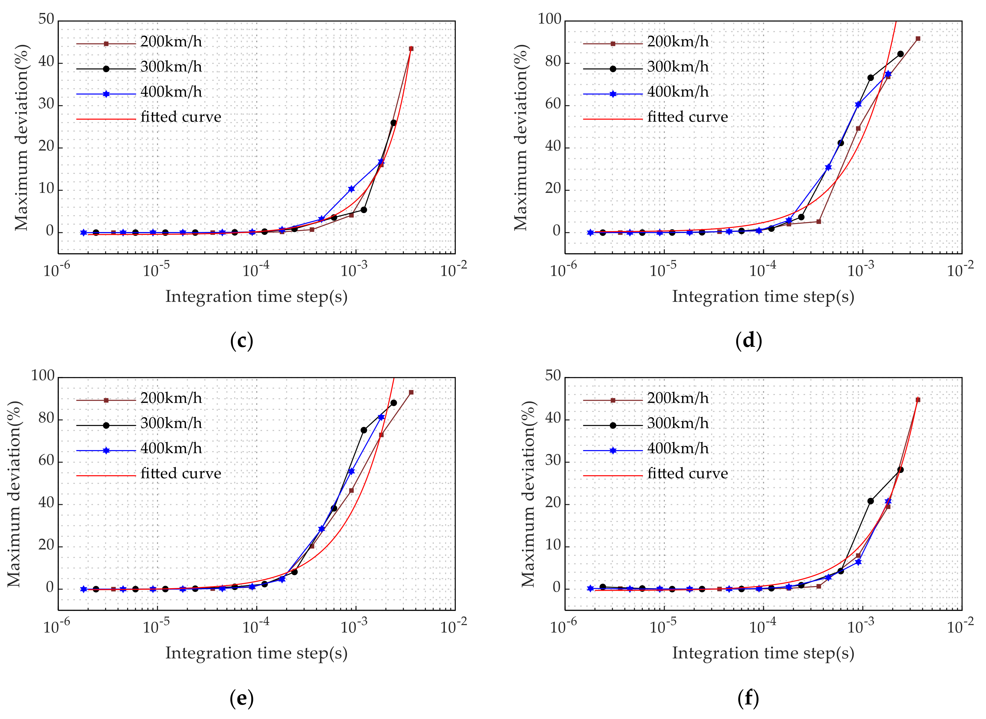
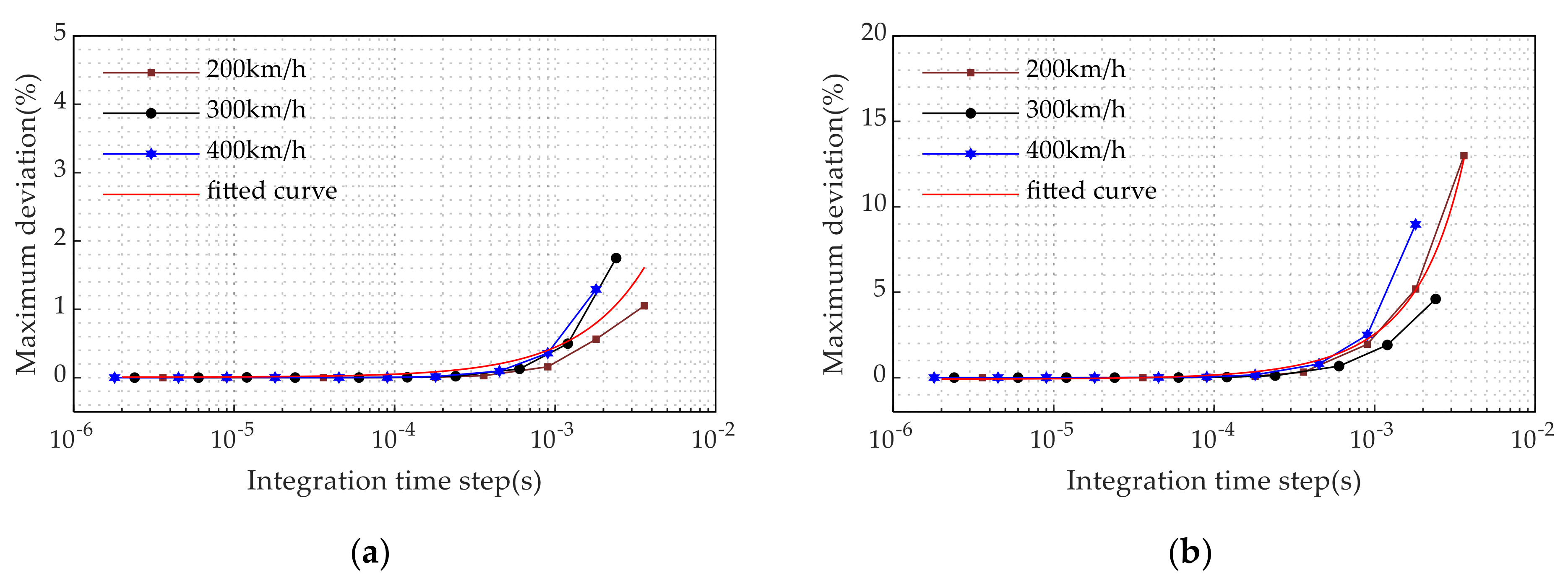
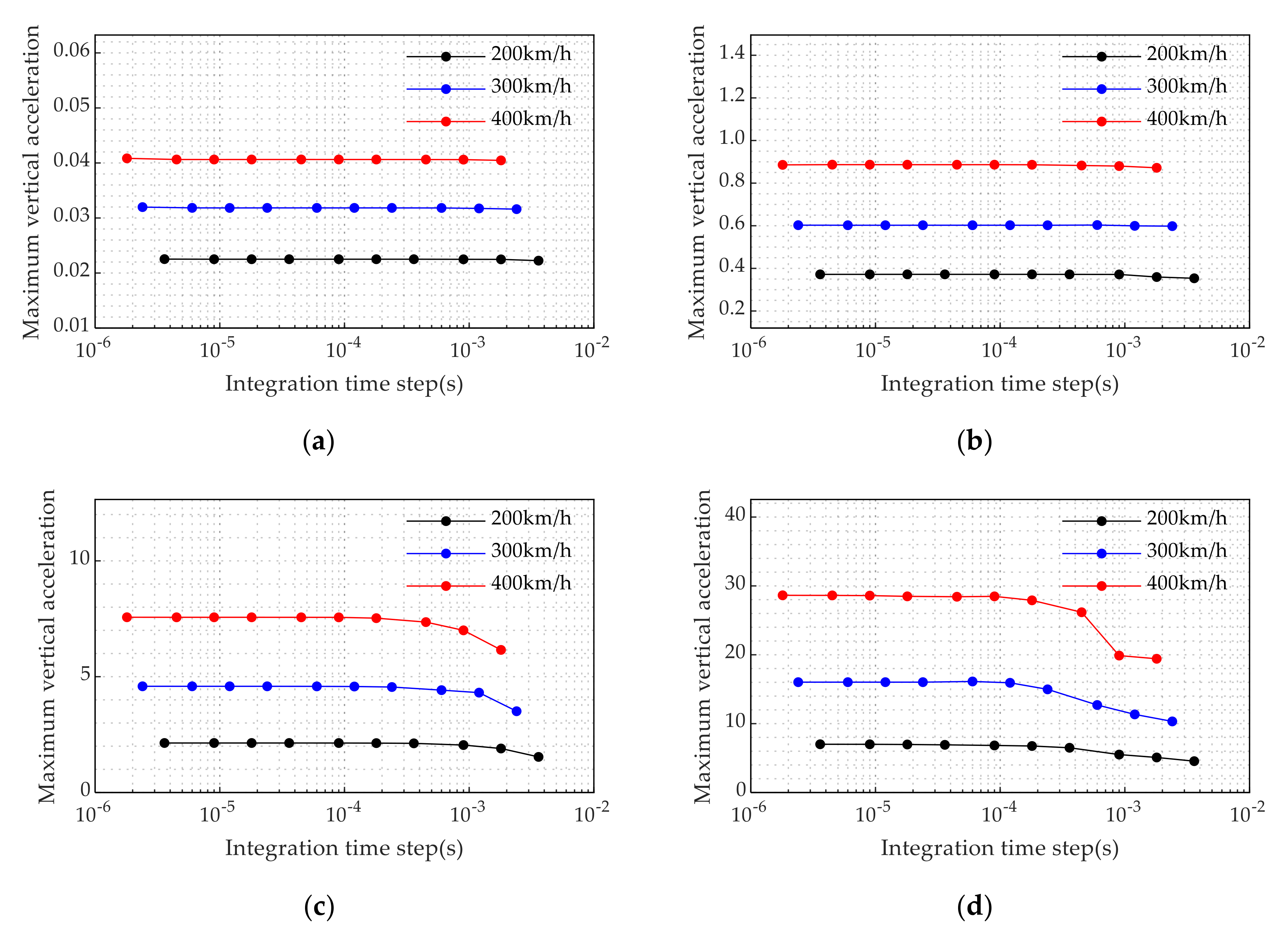
5.1.1. The Effect of Integration Time Step on Calculation Accuracy at Different Speeds

The influence of the integration time step on the calculation accuracy of the maximum vertical acceleration of each component at different speeds is shown in Figure 9a–f. It has little distinction that the effect of the integration time step on the calculation deviation of the maximum vertical acceleration at 200, 300 and 400 km/h. With the integration time step increasing, the increase in the calculation deviation of different components is quite different. The integration time step has a small influence on the maximum vertical acceleration of the car body. When the integration time step is less than 3.6 × 10⁻³ s, the maximum calculation deviation of vertical acceleration of the car body does not exceed 1.8% (Figure 9a). The integration time step has some influence on the calculation deviation of the maximum vertical acceleration of the bogie, and when the integration time step is 3.6 × 10⁻³ s, the maximum calculation deviation is close to 15% (Figure 9b). The integration time step has a great influence on the calculation deviation of wheel-sets and the bridge, and when the integration time step is 3.6 × 10⁻³ s, the maximum calculation deviation is close to 50% (Figure 9c–f). The integration time step has the greatest impact on the maximum vertical acceleration of the rail and track slab, and when the integration time step is 3.6 × 10⁻³ s, the maximum calculation deviation of the rail and track slab are close to 100% (Figure 9d–e).

Overall, it is obvious that the relationship between the calculation deviation of the maximum vertical acceleration and the integration time step for each component can be described as:

$$\eta = a·{\mathrm{e}}^{b·t}+c,$$

(36)

where, $\eta$ is calculation deviation of the maximum vertical acceleration; $a$, $b$ and $c$ are related parameter of the fitted function. The fitted curves of function for each component are shown in Figure 9, and the value of parameter for each component are shown in

Table 4. The Value of Parameters for the Function.

Parameter	a	b	c
Car body	28.13	15.43	−28.22
Bogie	10.88	217.19	−10.96
Wheel-sets	22.85	300.59	−23.32
Rail	1864.13	23.98	−1863.80
Track slab	1858.71	21.73	−1859.03
Bridge	119.93	89.86	−120.24

.

According to the calculation results, different components require different ranges of integration time step to ensure calculation deviation within 20%. The maximum integration time step of the car body can be appropriately greater than 3.6 × 10⁻³ s, and the range of the integration time step of the car body should be less than 5.2 × 10⁻³ s based on the fitted function (36). According to the calculation results, the range of the integration time step of the bogie should be less than 4 × 10⁻³ s; the ranges of the integration time step of the wheel-sets and bridge should be less than 2 × 10⁻³ s and 1 × 10⁻³ s, respectively; the ranges of the integration time step for the rail and track slab should be less than 3 × 10⁻⁴ s and 4 × 10⁻⁴ s, respectively.

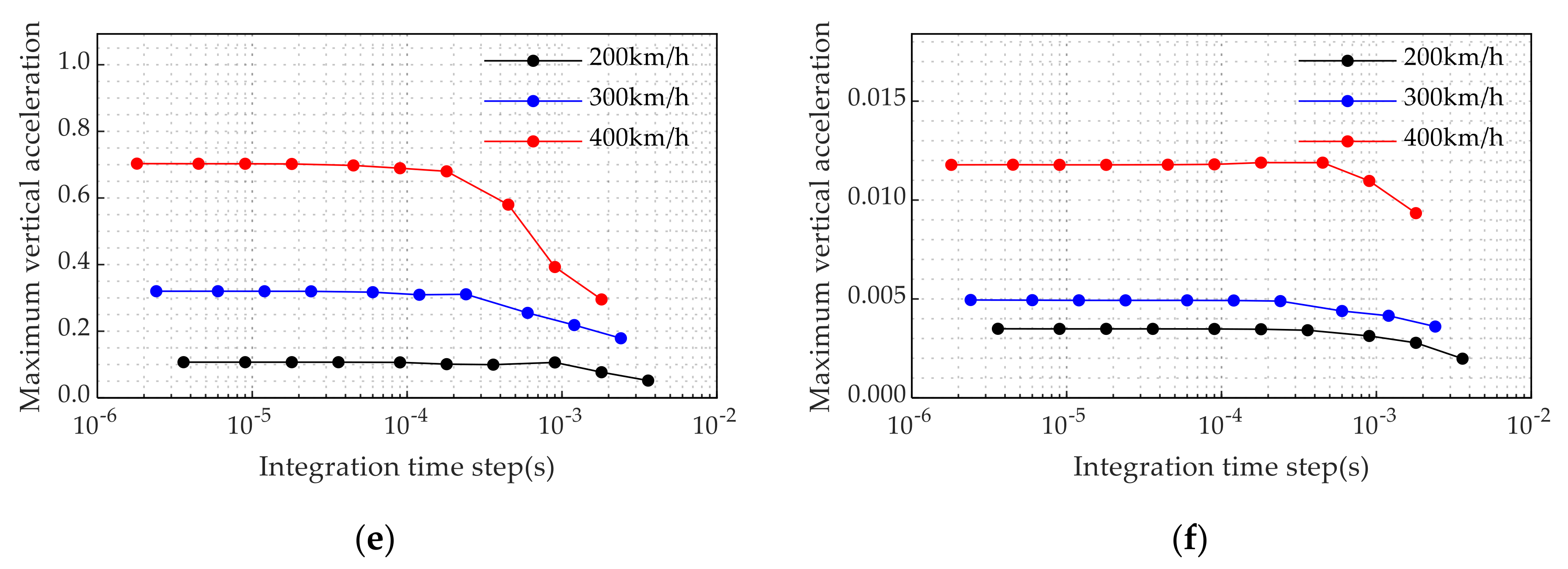
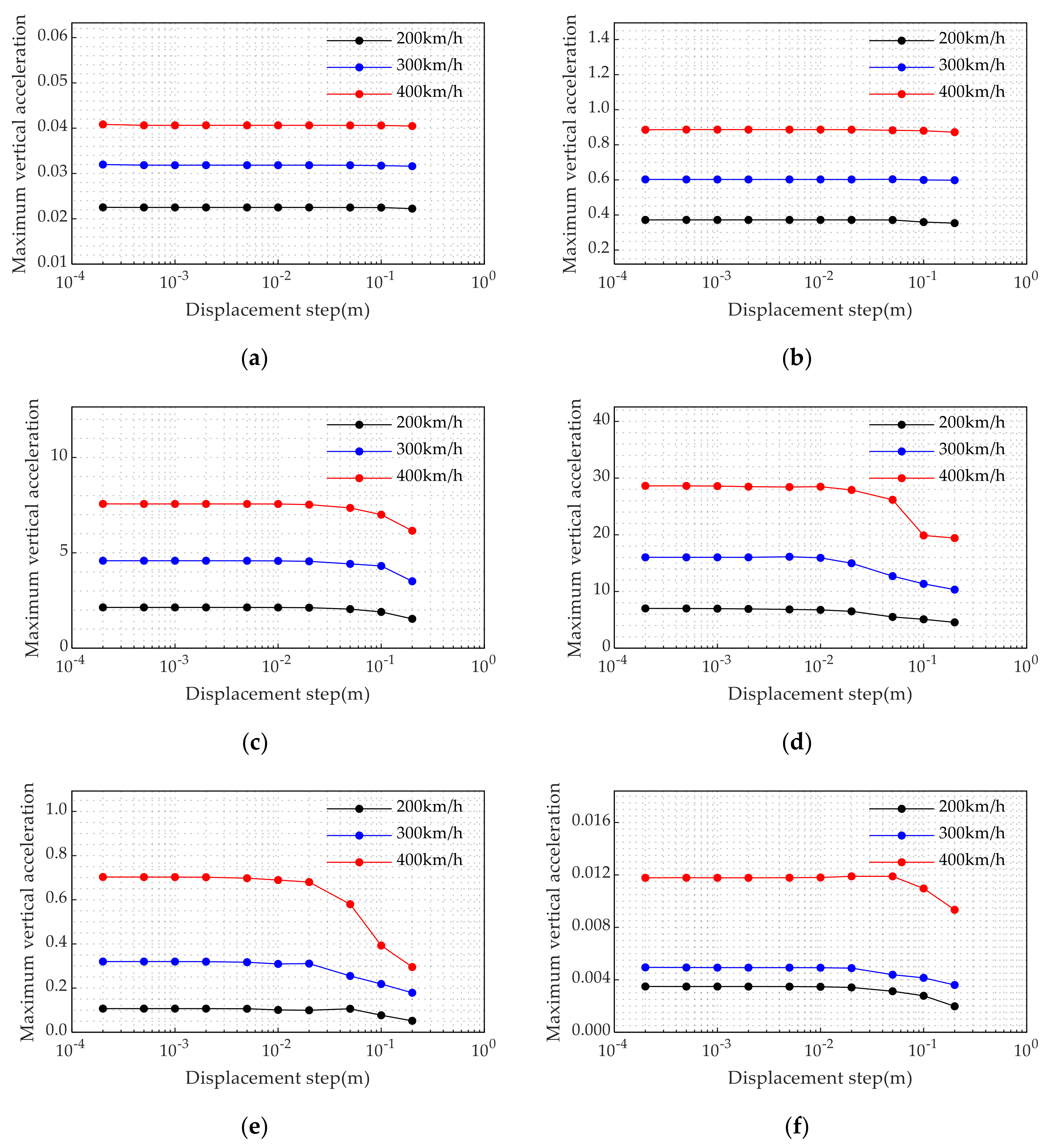
5.1.2. The Effect of the Integration Time Step on Calculation Stability at Different Speeds

The influence of the integration time step on the calculation stability of the maximum vertical acceleration of each component at different speeds is shown in Figure 10. The influence of the displacement step on each component at different speeds is shown in Figure 11. Obviously, the vehicle speed has a greater influence on the maximum vertical acceleration of each component. The results show that greater speed can cause greater vertical acceleration; however, the trend of maximum vertical acceleration of each component is similar at speeds of 200, 300 and 400 km/h. Comparing Figure 10 and Figure 11, the influence of the integration time step on the calculation stability of the maximum vertical acceleration for each component at different speeds is somewhat different. The integration time step gradually reduces at speeds of 200, 300 and 400 km/h when the maximum vertical acceleration of component starts to decrease, which means that higher speed requires a smaller integration time step to keep the calculation results stable. However, the value of the displacement step is more consistent at three speeds when the maximum vertical acceleration of each component decreases. This indicates that the mechanism of the influence of the integration time step on the calculation stability of the coupled system at different speeds is that displacement corresponding to the integration time step is different. Higher vehicle speed requires greater displacement step to keep calculation stability well.

Comparing Figure 10a–c, the value of the integration time step gradually increases when the maximum vertical acceleration of the wheel-sets, bogie, and car body begins to decrease. Comparing Figure 10d–f, the value of integration time step gradually increases when the maximum vertical acceleration of rail, track slab, and bridge begins to decrease. This is mainly because the wheel-rail interaction excites vibration of the vehicle-track-bridge coupled system when the high-speed vehicle passes the ballastless track. The high-frequency vibration gradually weakens as the vibration response is transmitted upward and downward from the wheel-rail contact position. Moreover, higher vibration frequency requires smaller an integration time step to ensure stable dynamic calculation.

In addition, compared with Figure 11a–f, it can be found that the displacement step has little effect on the calculation stability of the maximum vertical acceleration of the car body and bogie (Figure 11a,b), but it has a greater effect on the calculation stability of the maximum vertical acceleration of the wheel-sets, rail and track slab, and bridge (Figure 11c–f). When the displacement step does not exceed 0.2 m, the maximum vertical acceleration of the car body and bogie are 1.2% and 5.0%, respectively; the maximum vertical acceleration of the wheel-sets, rail, track slab, and bridge are 28.1%, 35.6%, 58.0% and 43.3%, respectively. When the displacement step is more than 0.02 m, the maximum vertical acceleration of the wheel-sets, rail, track slab and bridge begin to decrease, and the higher the speed is, the faster the acceleration decline. This is because higher vehicle speed requires a shorter time step to pass the same displacement step, and the vibration frequency is higher. Therefore, when the displacement step exceeds a certain limit, the higher the speed is, the faster the maximum vertical acceleration decreases.

According to the analysis of the results, different components require different ranges of displacement step to keep calculation stable. The maximum displacement step of the car body can be appropriately greater than 0.2 m (Figure 11a); the range of the displacement step for the bogie should be less than 0.2 m (Figure 11b); the range of the displacement step for wheel-sets should be less than 0.1 m (Figure 11c); the range of the displacement step for the rail, track slab and bridge all should be less than 0.02 m (Figure 11d–f). According to the formula $t_{\max }=x_{\max }/v$, the corresponding range of the integration time step at different speeds can be obtained.

In summary, the integration time step has a greater impact on the dynamic calculation of the VTB coupling system at different speeds. The results show that the disparity among the effect of the integration time step on calculation accuracy of each component at different speeds is small, and the effect on calculation stability of each component at different speeds depends on the effect of the displacement step. According to the calculation results from Figure 9, Figure 10 and Figure 11, the maximum of the integration time step for the bogie, wheel-sets, rail, track slab and bridge at speeds of 200, 300 and 400 km/h are shown in

Table 5. Maximum of the Integration Time Step for Each Component at Different Speeds (unit: s).

Component	200 km/h		300 km/h		400 km/h
	Limit of Accuracy	Limit of Stability	Limit of Accuracy	Limit of Stability	Limit of Accuracy	Limit of Stability
Car body	5.2 × 10−3	-	5.2 × 10−3	-	5.2 × 10−3	-
Bogie	4.0 × 10−3	3.6 × 10−3	4.0 × 10−3	2.4 × 10−3	4.0 × 10−3	1.8 × 10−3
Wheel-sets	2.0 × 10−3	1.8 × 10−3	2.0 × 10−3	1.2 × 10−3	2.0 × 10−3	9.0 × 10−4
Rail	1.0 × 10−3	3.6 × 10−4	1.0 × 10−3	2.4 × 10−4	1.0 × 10−3	1.8 × 10−4
Track slab	3.0 × 10−4	3.6 × 10−4	3.0 × 10−4	2.4 × 10−4	3.0 × 10−4	1.8 × 10−4
Bridge	4.0 × 10−4	3.6 × 10−4	4.0 × 10−4	2.4 × 10−4	4.0 × 10−4	1.8 × 10−4

, respectively. The maximum integration time step for the car body is obtained by the fitted curve. It is worth noting that the smaller integration time can obtain better accuracy and stability, so the range of the integration time step should be less than the maximum integration time step for each component.

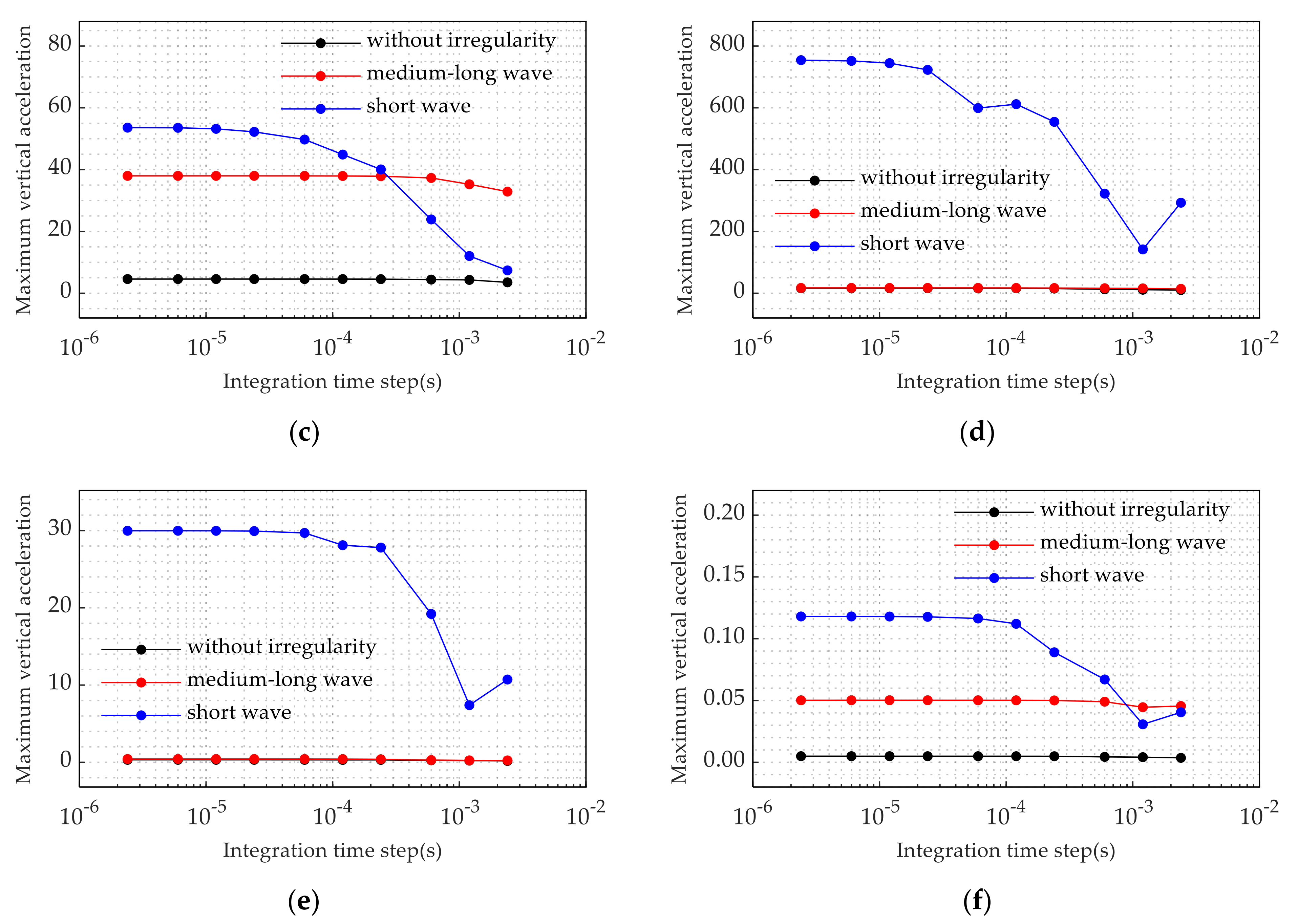
5.2. Effect under Different Track Irregularity States

In order to study the influence of the integration time step on the dynamic calculation of the vehicle-track-bridge coupled system under different track irregularity states, the vertical geometric states of the track are set as without track irregularity, track short wave irregularity, and track medium-long wave irregularity. The speed is 300 km/h, and the displacement steps are 1/5, 1/10, 1/20, 1/50, 1/100, 1/200, 1/500, 1/1000, 1/2000, 1/5000 m, and the corresponding integration time steps refer to Table 3.

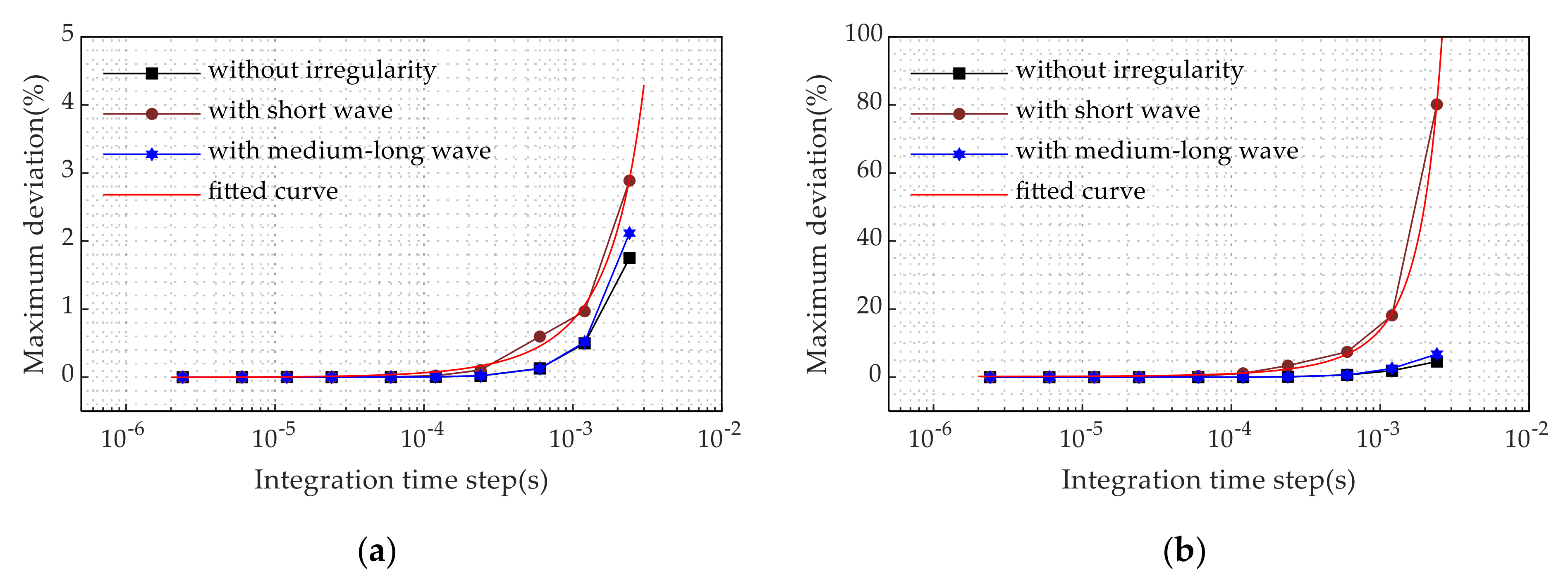
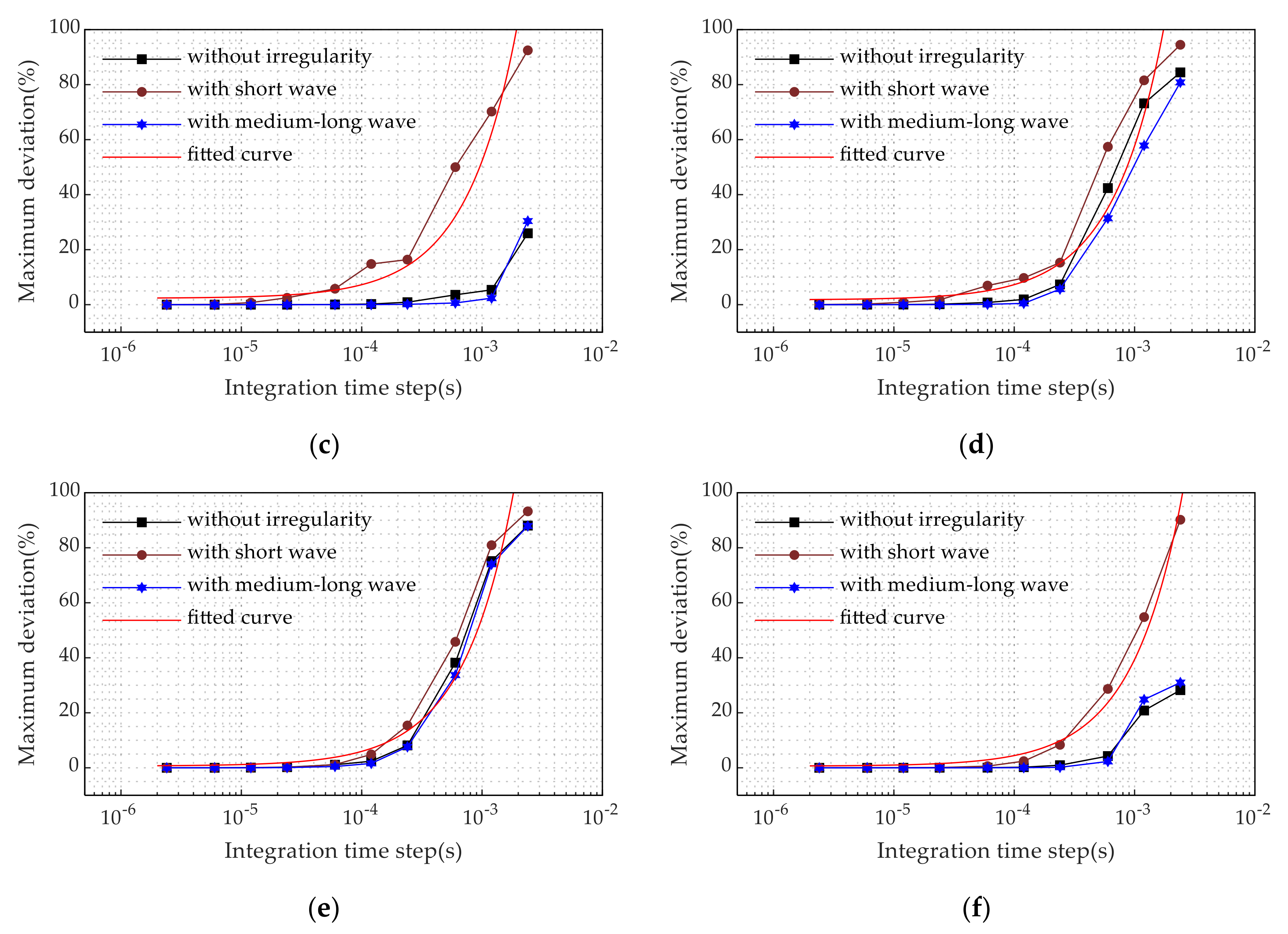
5.2.1. The Effect of the Integration Time Step on Calculation Accuracy under Different Track Irregularity States

The influence of the integration time step on the calculation accuracy of the maximum vertical acceleration of each component under different track regularity states is shown in Figure 12. The influence of the integration time step on the calculation accuracy of the maximum vertical acceleration of the car body, bogie, and wheel-sets is quite different under different track irregularity states. Compared with the without track irregularity state, the maximum calculation deviation of the car body under track short wave irregularity increases from 1.8% to 2.9% (Figure 12a). However, the calculation deviation of the maximum vertical acceleration of the bogie and wheel-sets improve greatly under the track short wave irregularity state. Among them, the maximum calculation deviation of the bogie increases from 4.6% to 80.2% (Figure 12b), and that of wheel-sets increases from 25.9% to 84.5% (Figure 12c). The influence of the integration time step on the calculation accuracy of the maximum vertical acceleration of the rail, track slab and bridge of the system is quite different under different track irregularity states. Compared the calculation deviation under the without track irregularity state, the calculation deviation of the maximum vertical acceleration of the rail is slightly increased, and the maximum calculation deviation increases from 84.4% to 94.5% (Figure 12d). The calculation deviation of the maximum vertical acceleration of the track slab shows little change, and the maximum calculation deviation increases from 88.1% to 93.2% (Figure 12e). However, the calculation deviation of the maximum vertical acceleration of the bridge greatly improved, and the maximum calculation deviation increases from 28.2% to 90.2% (Figure 12f).

The relationship between the calculation deviation of the maximum vertical acceleration and the integration time step under two track irregularity states also fits the function (36). The fitted curves of function for each component under the track short irregularity wave state are shown in Figure 12. The functions for each component under the track medium-long irregularity are consistent with that under the without track irregularity state, whose parameters can be referred to in Table 4. The value of parameters for each component under the different track irregularity states are shown in

Table 6. The Value of Parameters for the Function under the Track Short Wave Irregularity State.

Parameter	a	b	c
Car body	1.45	459.56	−1.45
Bogie	8.04	998.63	−7.85
Wheel-sets	1908.13	25.82	−1905.80
Rail	2128.93	25.94	−2127.17
Track slab	2050.82	25.94	−2050.17
Bridge	1318.25	28.99	−1317.64

.

According to the analysis of the results, different components require different ranges of the integration time step to ensure calculation deviation within 20%. The maximum integration time step of the car body under the track short wave irregularity state can be appropriately greater than 2.4 × 10⁻³ s, and the range of the integration time step of the car body should be less than 5.9 × 10⁻³ s based on the fitted function (36); the range of the integration time step for the bogie should not exceed 1.5 × 10⁻³ s; the range of the integration time step for the wheel-sets, rail and track slab should be less than 2.4 × 10⁻⁴ s, and the range of the integration time step for the bridge should be less than 4 × 10⁻⁴ s. The range of the integration time step for the car body, bogie, wheel-sets, rail, track slab and bridge are consistent with that under the without track irregularity state.

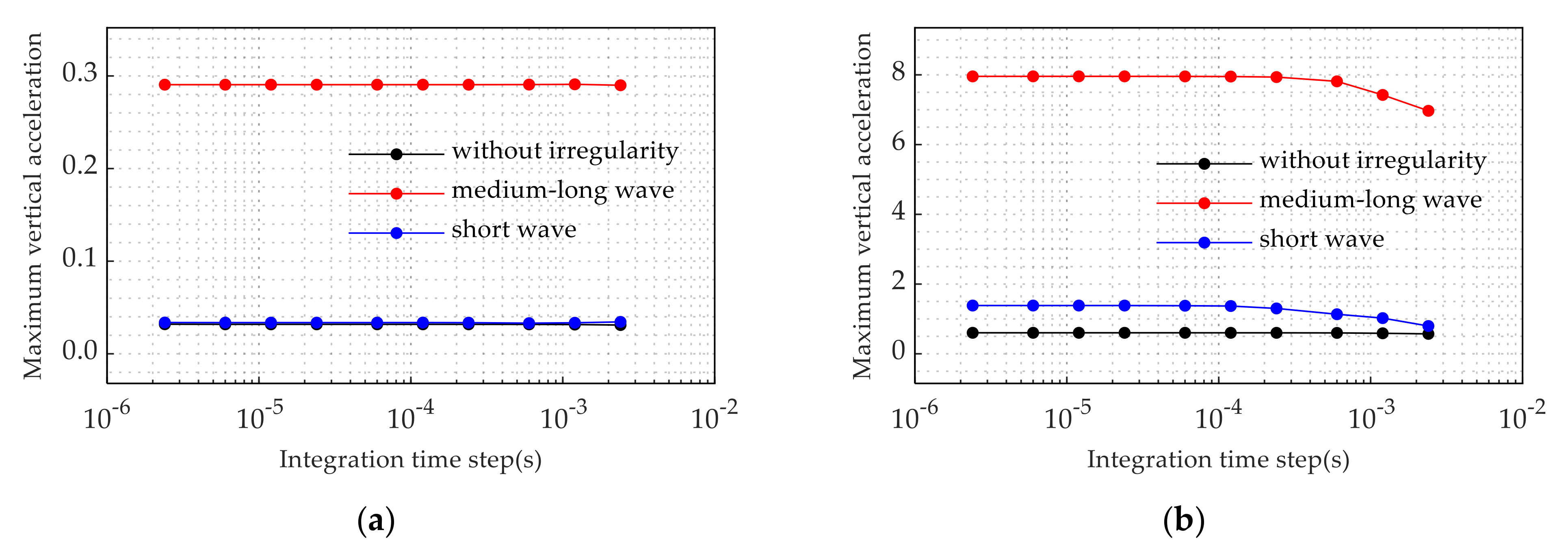
5.2.2. The Effect of the Integration Time Step on Calculation Stability under Different Track Irregularity States

The influence of the integration time step on the maximum vertical acceleration of each component under different track irregularity states is shown in Figure 13. The maximum vertical acceleration of the car body, bogie and wheel-sets all increase significantly under track medium-long wave irregularity. The maximum vertical acceleration of the car body and bogie shows little change under track short wave irregularity, while that of wheel-sets shows a significant increase. The maximum vertical acceleration of the car body both maintains a good stability under the track medium-long wave irregularity state and the track short wave irregularity state (Figure 13a). With the integration time step increasing, the maximum vertical acceleration of the bogie shows a downward trend under the two track irregularity states, and the drop of amplitudes are 12.4% and 42.4%, respectively (Figure 13b). The maximum vertical acceleration of the wheel-sets shows a downward trend under the two track irregularity states, and the decline amplitude under track short wave irregularity state is much greater than that under the track medium–long wave irregularity state, and the drops of amplitude are 13.4% and 86.2%, respectively (Figure 13c). The integration time step has little effect on the calculation stability of the maximum vertical acceleration of the rail, track slab and bridge under the track medium-long wave irregularity state, and maximum drops of amplitude are 17.2%, 42.6% and 11.2%, respectively. The integration time step has a great influence on the calculation stability of the maximum vertical acceleration of the rail, track slab and bridge under the track short wave irregularity state. With the increase in the integration time step, the maximum vertical acceleration of the rail, track slab and bridge all show a significant decline, and the maximum drops of amplitude are 81.2%, 75.3% and 74.0%, respectively.

Moreover, the maximum vertical acceleration of wheel-sets under the track short wave irregularity state drops rapidly with the integration time step increasing, until it is close to the value that shown without track irregularity. This indicates that, if the integration time step is larger, the influence of track short wave irregularity on the maximum vertical acceleration of the wheel-sets approaches zero. The maximum vertical accelerations of the rail, track slab and bridge under the track medium-long wave irregularity state show a small increase, while that the under track short wave irregularity state increase significantly. The influence of the integration time step on calculation stability of the maximum vertical acceleration of the rail, track slab and bridge show great differences under the two track irregularity states.

According to the analysis of the results, different components require different ranges of displacement step to keep the calculation stable. The maximum integration time step for the car body can be appropriately greater than 2.4 × 10⁻³ s. The range of integration time step of the bogie and wheel-sets under track medium-long wave irregularity should be less than 2 × 10⁻³ s and 2 × 10⁻³ s. The range of the integration time step of the bogie and wheel-sets under the track short wave irregularity state should be less than 3 × 10⁻⁴ s and 6 × 10⁻⁵ s, respectively. The range of the integration time step of the rail, track slab, and bridge under medium-long wave irregularity should be less than 1.5 × 10⁻³, 3 × 10⁻⁴ and 1 × 10⁻³ s, respectively. Under the track short wave irregularity state, the range of the integration time step of the rail, track slab and bridge should be less than 3 × 10⁻⁵, 2.4 × 10⁻⁴ and 1.5 × 10⁻⁴ s, respectively.

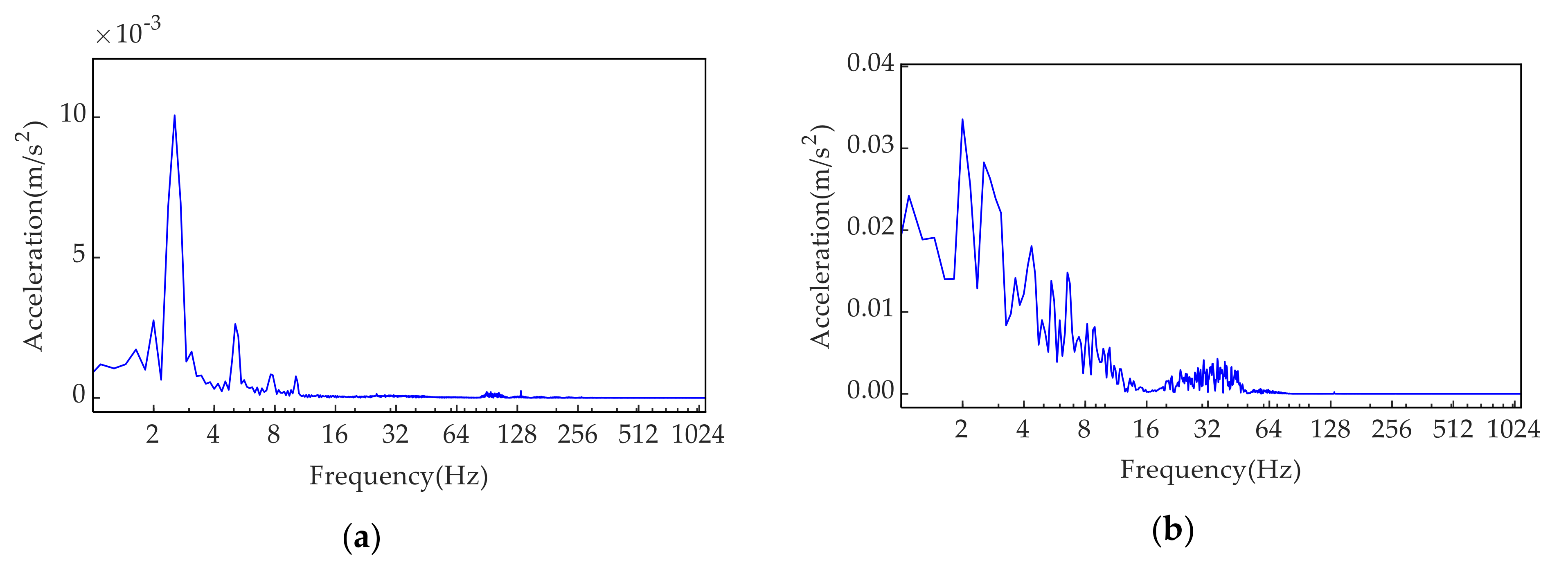
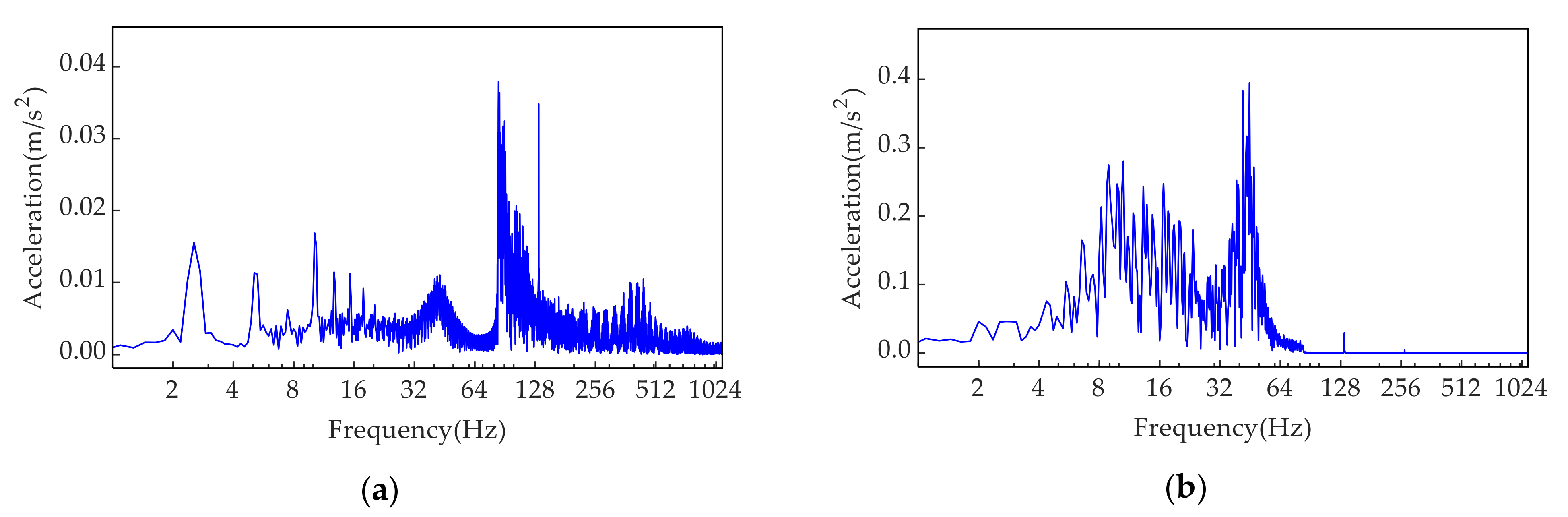
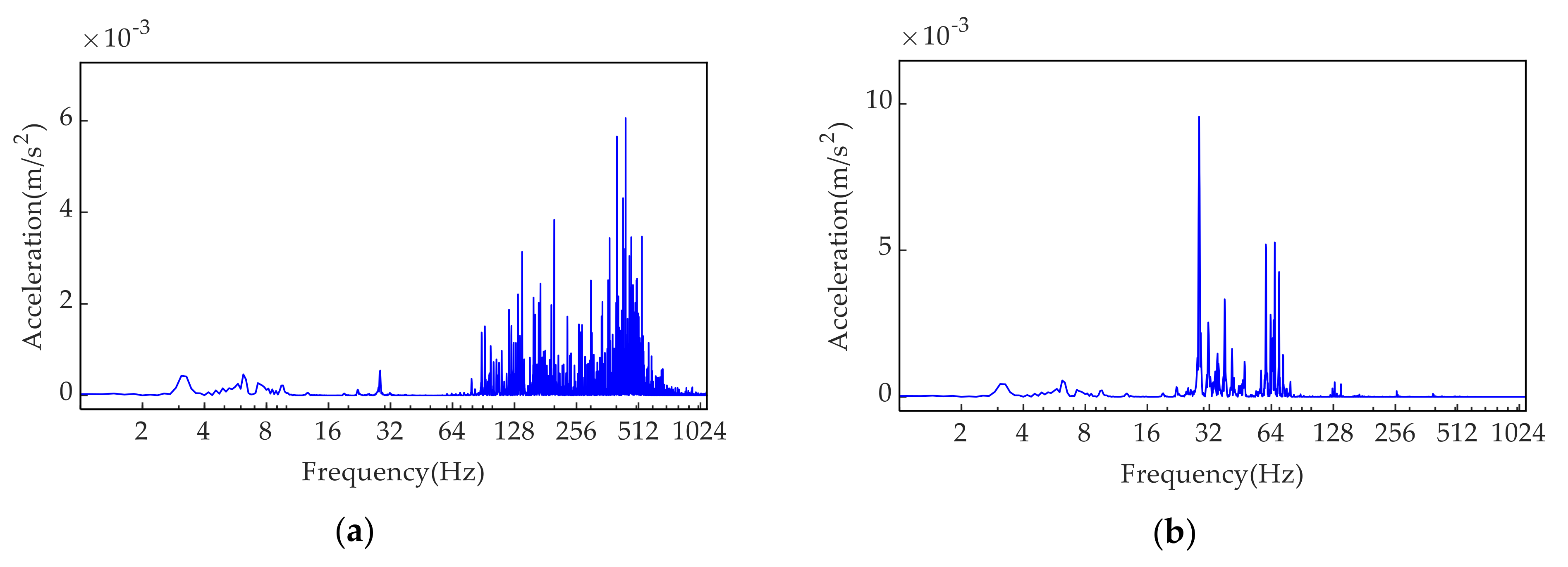
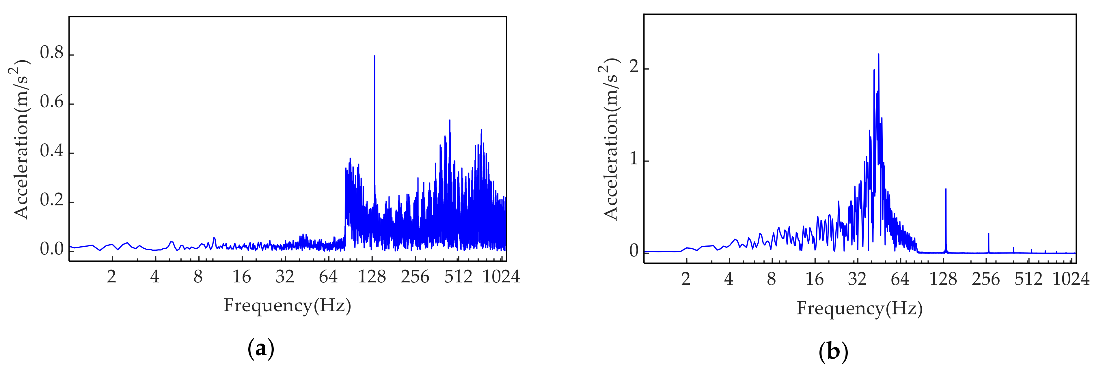
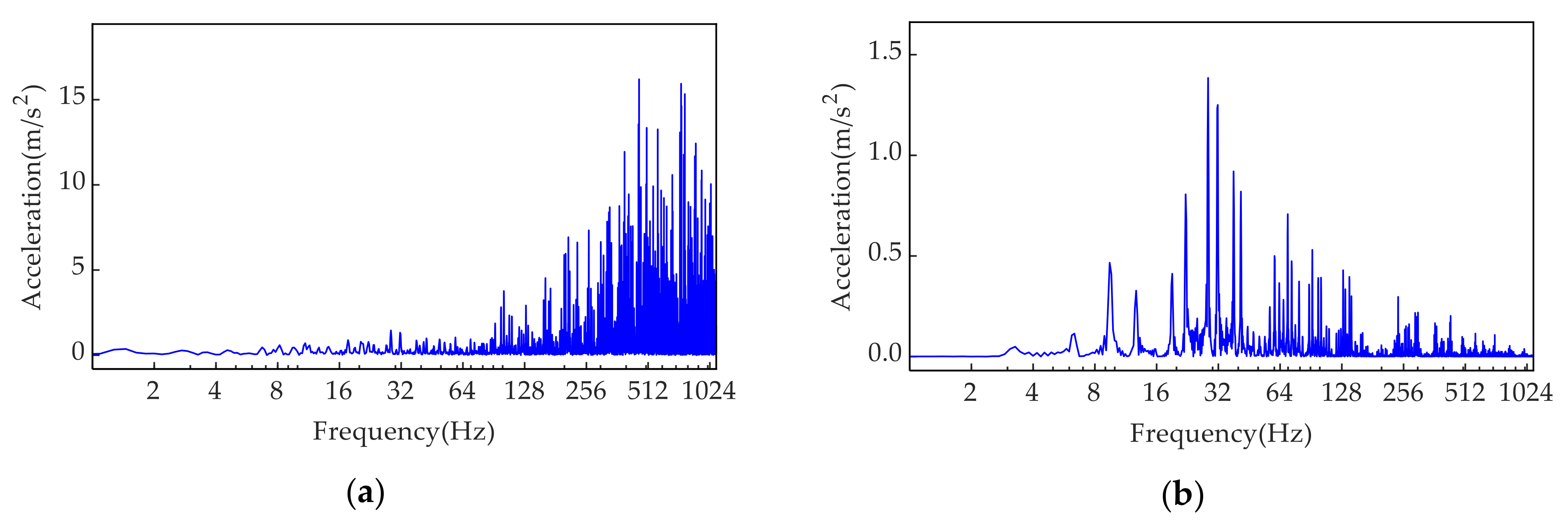
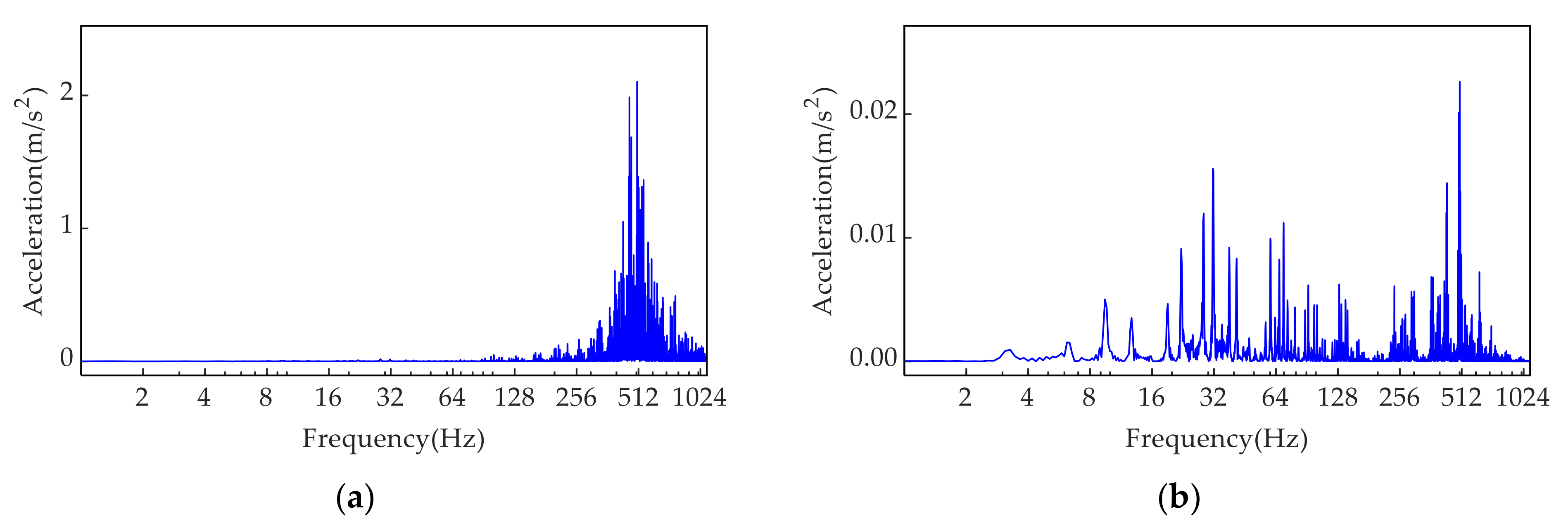
5.2.3. Spectrum Characteristic of Components under Different Track Irregularity States

From the definition of the transfer function, it can be considered that the wavelength corresponding to the peak of the amplitude-frequency characteristic curve of the transfer function is the sensitive wavelength [35]. The sensitive wavelength can be obtained by $\lambda =v/f$, and the displacement step can be obtained from $\Delta s=v·\Delta t$. To ensure the stability of the calculation results, the displacement step is less than the sensitive wavelength of the structure; that is, the integration time step should be less than a certain limit. When the displacement step is 1/5000 m and the speed is 300 km/h, the frequency characterizations of the vertical acceleration under track short wave irregularity and track medium-long wave irregularity are shown in Figure 14, Figure 15, Figure 16, Figure 17, Figure 18 and Figure 19, respectively.

Comparing Figure 14, Figure 15 and Figure 16, it can be seen that the vertical vibration of the car body is mainly low-frequency vibration, and the dominant frequencies and vibration amplitudes of the vibration of the car body, bogie, and wheel-sets gradually increase. This indicates that the sensitive wavelength of the car body is relatively large ($\lambda =v/f$), the sensitive wavelengths of the bogie and wheel-sets gradually decrease, and the vibration response of the wheel-sets, bogie and car body gradually weaken during the transmission process. Comparing Figure 17, Figure 18 and Figure 19, it can be seen that the vibration frequencies of the rail, track slab, and bridge are higher, which indicates that the sensitive wavelength of the rail, track slab, and bridge is smaller.

In addition, it can be seen that the vibration amplitudes of the car body, bogie and wheel-sets under medium-long wave irregularity are more than that under track short wave irregularity, while the vibration amplitudes of the rail and track slab under track short wave irregularity are more than that under track medium-long wave irregularity. This is because the spatial frequency of track irregularity is $f={\lambda }^{-1}$, short wave irregularity mainly excites high-frequency vibration, and medium-long wave irregularity mainly excites low-frequency vibration. This indicates that the car body, bogie and wheel-sets have larger sensitive wavelengths and are sensitive to medium-long waves, however, rail and track slab have smaller sensitive wavelengths and are sensitive to short waves. To ensure that the displacement step is less than the sensitive wavelength of the component, the displacement step should meet $\Delta x\le \lambda /n=v/nf$ (n takes 3~5), namely the integration time step should meet $\Delta t=\Delta x/v\le 1/nf$. Because the sensitive wavelength of the car body, bogie, wheel-sets, rail, track slab and bridge gradually decrease, the effect of track medium-long wave irregularity on calculation stability of the car body, bogie, wheel-sets, rail, track slab and bridge gradually decrease, while the effect under the track short wave irregularity state gradually increases. It follows that the larger the vibration frequency is, the smaller the range of integration time step is for dynamic calculation to maintain calculation stability, which is consistent with the analysis result (chapter 5.1.2) that the maximum integration time step of the car body, bogie, wheel-sets, rail, track slab and bridge gradually increases.

In summary, the integration time step has a greater impact on the dynamic calculation of the VTB coupling system under different track irregularities states. The disparity among the effect of the integration time step on calculation accuracy and calculation stability of the calculation under the track irregularity states is different. According to the calculation results from Figure 12 and Figure 13, different components have different sensitivities to the integration time step, and the maximum of the integration time step for bogie, wheel-sets, rail, track slab and bridge under different track irregularity states at a speed of 300 km/h are shown in

Table 7. Maximum of the Integration Time Step for Each Component under Different Track Irregularity States (unit: s).

Component	Without Track Irregularity		Short Wave Irregularity		Medium-Long Wave Irregularity
	Limit of Accuracy	Limit of Stability	Limit of Accuracy	Limit of Stability	Limit of Accuracy	Limit of Stability
Car body	5.2 × 10−3	-	5.9 × 10−3	-	5.2 × 10−3	-
Bogie	4.0 × 10−3	2.4 × 10−3	1.5 × 10−3	3.0 × 10−4	4.0 × 10−3	2.0 × 10−3
Wheel-sets	2.0 × 10−3	1.2 × 10−3	2.4 × 10−4	6.0 × 10−5	2.0 × 10−3	2.0 × 10−3
Rail	1.0 × 10−3	2.4 × 10−4	2.4 × 10−4	3.0 × 10−5	1.0 × 10−3	1.5 × 10−3
Track slab	3.0 × 10−4	2.4 × 10−4	2.4 × 10−4	2.4 × 10−4	3.0 × 10−4	3.0 × 10−4
Bridge	4.0 × 10−4	2.4 × 10−4	4.0 × 10−4	1.5 × 10−4	4.0 × 10−4	1.0 × 10−3

. The maximum integration time step for the car body is obtained by the fitted curve. It is worth noting that smaller integration time can obtain better accuracy and stability, so the range of the integration time step should be less than the maximum integration time step for each component.

6. Conclusions

In this paper, a vehicle-train-bridge coupled model is established. The influence of the integration time step on calculation accuracy, calculation stability of finite element simulation is studied, and the influence mechanism of the integration time step on the vibration response of each component under different track irregularity states is analyzed through the spectral characteristic of sensitive wavelength. The main conclusions are shown as follows:

(1)

The integration time step has a great influence on the calculation accuracy of each component, but the disparity among the effect of the integration time step on the calculation accuracy at different speeds is very small. The integration time step has a greater influence on the calculation deviation of the maximum vertical acceleration of the rail and track slab. The range of the integration time step of the car body, bogie, wheel-sets, rail, track slab and bridge should be less than 5.2 × 10⁻³, 4 × 10⁻³, 2 × 10⁻³, 1 × 10⁻³, 3 × 10⁻⁴ and 4 × 10⁻⁴ s, respectively.

(2)

The effect of the integration time step on the calculation stability of the maximum vertical acceleration of each component at different speeds is somewhat different, but the effect of the displacement step on the maximum vertical acceleration of each component at three speeds is more consistent. Higher speed requires a smaller integration time step to keep the calculation results stable. The mechanism of the effect of the integration time step on the calculation stability of the vehicle-track-bridge coupled system is that the corresponding displacement at the integration time step is different. The range of the displacement step of the bogie, wheel-sets, rail, track slab and bridge should be less than 0.2, 0.1, 0.02, 0.02 and 0.02 m, respectively.

(3)

The calculation deviation of the maximum vertical acceleration of the car body, bogie, wheel-sets, rail, track slab and bridge under track medium-long wave irregularity is more consistent with that under without track irregularity; however, the calculation deviation of the maximum vertical acceleration of the car body, wheel-sets and bridge under track short wave irregularity are greatly increased compared with that under without track irregularity. The range of integration time step of the car body, bogie, wheel-sets, rail, track slab and bridge under the track short wave irregularity state should be less than 5.9 × 10⁻³, 1.5 × 10⁻³, 2.4 × 10⁻⁴, 2.4 × 10⁻⁴, 2.4 × 10⁻⁴ and 4 × 10⁻⁴ s, respectively.

(4)

The effect of the integration time step on the calculation stability of the maximum vertical acceleration of each component under the track medium-long wave irregularity state is little, however, while the maximum vertical acceleration of the wheel-sets, rail, track slab and bridge under track short wave irregularity all show a significant declining trend. The range of the integration time step of the bogie, wheel-sets, rail, track slab and bridge under the track medium-long wave irregularity state should be less than 2 × 10⁻³, 2 × 10⁻³, 1.5 × 10⁻³, 3 × 10⁻⁴ and 1 × 10⁻³ s, respectively, and the range under the track short wave irregularity state should be less than 3 × 10⁻⁴, 6 × 10⁻⁵, 3 × 10⁻⁵, 2.4 × 10⁻⁴ and 1.5 × 10⁻⁴ s, respectively.

(5)

Short wave irregularity mainly excites high-frequency vibration, and medium-long wave irregularity mainly excites low-frequency vibration. The larger the vibration frequency is, the smaller the range of the integration time step is for dynamic calculation to maintain calculation stability.

References

1. Xu, J.; Wang, P.; An, B.; Ma, X.; Chen, R. Damage detection of ballastless railway tracks by the impact-echo method. Proc. Inst. Civ. Eng. Transp. 2018, 171, 106–114. [Google Scholar] [CrossRef]
2. Zhu, S.; Fu, Q.; Cai, C.; Spanos, P.D. Damage evolution and dynamic response of cement asphalt mortar layer of slab track under vehicle dynamic load. Sci. China Ser. E Technol. Sci. 2014, 57, 1883–1894. [Google Scholar] [CrossRef]
3. Han, J.; Zhao, G.; Xiao, X.; Jin, X. Effect of cement asphalt mortar damage location on dynamic behavior of high-speed track. Adv. Mech. Eng. 2018, 10. [Google Scholar] [CrossRef] [Green Version]
4. Liang, H.; Liu, P.; Wang, T.; Wang, H.; Zhang, K.; Cao, Y.; An, D. Influence of wheel polygonal wear on wheel-rail dynamic contact in a heavy-haul locomotive under traction conditions. Proc. Inst. Mech. Eng. Part F J. Rail Rapid Transit 2020. [Google Scholar] [CrossRef]
5. Shan, Y.; Zhou, S.; Zhou, H.; Wang, B.; Zhao, Z.; Shu, Y.; Yu, Z. Iterative Method for Predicting Uneven Settlement Caused by High-Speed Train Loads in Transition-Zone Subgrade. Transp. Res. Rec. J. Transp. Res. Board 2017, 2607, 7–14. [Google Scholar] [CrossRef]
6. Liu, J.; He, Y.; Zhang, J.; Hong, J.; Wen, X.; Xiao, J.; Wang, F.; Zheng, X. Polymer Injection Rehabilitation Technology for Lifting Differential Settlement of Turnout Ballastless Track. In Proceedings of the MATEC Web of Conferences, Cape Town, South Africa, 19–21 November 2018. [Google Scholar]
7. Zhai, W. The vertical model of vehicle-track system and its coupling dynamics. J. China Railw. Soc. 1992, 3, 10–21. [Google Scholar]
8. Xin, T.; Wang, P.; Ding, Y. Effect of Long-Wavelength Track Irregularities on Vehicle Dynamic Responses. Shock. Vib. 2019, 2019, 1–11. [Google Scholar] [CrossRef]
9. Gao, J.; Zhai, W.; Guo, Y. Wheel–rail dynamic interaction due to rail weld irregularity in high-speed railways. Proc. Inst. Mech. Eng. Part F J. Rail Rapid Transit 2018, 232, 249–261. [Google Scholar] [CrossRef]
10. Palomo, M.L.; Barceló, F.R.; Llario, F.R.; Herráiz, J.R. Effect of vehicle speed on the dynamics of track transitions. J. Vib. Control 2017. [Google Scholar] [CrossRef]
11. Li, T.; Su, Q.; Kaewunruen, S. Influences of dynamic material properties of slab track components on the train-track vibration interactions. Eng. Fail. Anal. 2020, 115, 104633. [Google Scholar] [CrossRef]
12. Yang, H.; Chen, Z.; Zhang, H.; Fan, J. Dynamic Analysis of Train-Rail-Bridge Interaction considering Concrete Creep of a Multi-Span Simply Supported Bridge. Adv. Struct. Eng. 2014, 17, 709–720. [Google Scholar] [CrossRef]
13. Ling, L.; Dhanasekar, M.; Thambiratnam, D.P. Dynamic response of the train–track–bridge system subjected to derailment impacts. Veh. Syst. Dyn. 2017, 56, 638–657. [Google Scholar] [CrossRef]
14. Zhai, W.M.; Wang, Q.C.; Lu, Z.W.; Wu, X.S. Dynamic effects of vehicles on tracks in the case of raising train speeds. Proc. Inst. Mech. Eng. Part F J. Rail Rapid Transit 2001, 215, 125–135. [Google Scholar] [CrossRef]
15. Zhai, W.; Xia, H.; Cai, C.; Gao, M.; Li, X.; Guo, X.; Zhang, N.; Wang, K. High-speed train–track–bridge dynamic interactions—Part I: Theoretical model and numerical simulation. Int. J. Rail Transp. 2013, 1, 3–24. [Google Scholar] [CrossRef]
16. Chen, Z.; Zhai, W.; Yin, Q. Analysis of structural stresses of tracks and vehicle dynamic responses in train–track–bridge system with pier settlement. Proc. Inst. Mech. Eng. Part F J. Rail Rapid Transit 2018, 232, 421–434. [Google Scholar] [CrossRef]
17. Chen, Z.; Zhai, W.; Cai, C.; Sun, Y. Safety threshold of high-speed railway pier settlement based on train-track-bridge dynamic interaction. Sci. China Ser. E Technol. Sci. 2014, 58, 202–210. [Google Scholar] [CrossRef]
18. Xiao, X.; Yan, Y.; Chen, B. Stochastic dynamic analysis for vehicle-track-bridge system based on probability density evolution method. Eng. Struct. 2019, 188, 745–761. [Google Scholar] [CrossRef]
19. A Zakeri, J.; Feizi, M.M.; Shadfar, M.; Naeimi, M. Sensitivity analysis on dynamic response of railway vehicle and ride index over curved bridges. Proc. Inst. Mech. Eng. Part K J. Multi-body Dyn. 2016, 231, 266–277. [Google Scholar] [CrossRef]
20. Xia, H.; Guo, W.; Zhang, N.; Sun, G. Dynamic analysis of a train–bridge system under wind action. Comput. Struct. 2008, 86, 1845–1855. [Google Scholar] [CrossRef]
21. Olmos, J.M.; Astiz, M.A. Analysis of the lateral dynamic response of high pier viaducts under high-speed train travel. Eng. Struct. 2013, 56, 1384–1401. [Google Scholar] [CrossRef]
22. Xia, H.; Han, Y.; Zhang, N.; Guo, W. Dynamic analysis of train–bridge system subjected to non-uniform seismic excitations. Earthq. Eng. Struct. Dyn. 2006, 35, 1563–1579. [Google Scholar] [CrossRef]
23. Zhai, W.; Wang, K.; Cai, C. Fundamentals of vehicle–track coupled dynamics. Veh. Syst. Dyn. 2009, 47, 1349–1376. [Google Scholar] [CrossRef]
24. Zhu, Z.; Gong, W.; Wang, L.; Li, Q.; Bai, Y.; Yu, Z.; Harik, I.E. An efficient multi-time-step method for train-track-bridge interaction. Comput. Struct. 2018, 196, 36–48. [Google Scholar] [CrossRef]
25. Jin, Z.; Hu, C.; Pei, S.; Liu, H. An integrated explicit–implicit algorithm for vehicle–rail–bridge dynamic simulations. Proc. Inst. Mech. Eng. Part F J. Rail Rapid Transit 2018, 232, 1895–1913. [Google Scholar] [CrossRef]
26. Zhai, W. Vehicle-Track Coupled Dynamics, 4th ed.; Science Press: Beijing, China, 2015; p. 41. [Google Scholar]
27. Xu, Q.; Chen, X.; Yan, B.; Guo, W. Study on vibration reduction slab track and adjacent transition section in high-speed railway tunnel. J. Vibroeng. 2015, 17, 905–916. [Google Scholar]
28. Sato, Y. Study on High-Frequency Vibrations in Track Operated with High-Speed Trains; Railway Technical Research Institute, Quarterly Reports; National Academies of Sciences, Engineering, and Medicine: Washington, DC, USA, 1977; p. 18. [Google Scholar]
29. Zeng, Q. The principle of total potential energy with stationary value in elastic system dynamics. J. Hua Zhong Univ. Sci. Technol. 2000, 1–3, 113163909. [Google Scholar]
30. Lou, P.; Zeng, Q.-Y. Formulation of Equations of Motion for a Simply Supported Bridge under a Moving Railway Freight Vehicle. Shock. Vib. 2007, 14, 429–446. [Google Scholar] [CrossRef]
31. Lou, P. Finite element analysis for train–track–bridge interaction system. Arch. Appl. Mech. 2007, 77, 707–728. [Google Scholar] [CrossRef]
32. Wu, Y.-S.; Yang, Y.-B. Steady-state response and riding comfort of trains moving over a series of simply supported bridges. Eng. Struct. 2003, 25, 251–265. [Google Scholar] [CrossRef]
33. Newmark, N.M. A method of computation for stuctural dynamics. J. Eng. Mech. Div. 1959, 85, 67–94. [Google Scholar] [CrossRef]
34. Lou, P.; Zeng, Q. Formulation of equations of vertical motion for vehicle-track-bridge system. J. China Railw. Soc. 2004, 5, 71–80. [Google Scholar]
35. Xu, J. Study on Random Vibration Analysis of High Speed Vehicle track Coupling System and Evaluation Method of Track Irregularity. Ph.D. Thesis, Southwest Jiaotong University, Chengdu, China, 2016. [Google Scholar]
Figure 1. The mechanical model diagram of the high-speed train submodel.
Mathematics 09 00431 g001
Figure 2. Typical section of the China Railway Track System I type slab track on the bridge: (a) schematic diagram of the solid section; (b) section size of one side of the structure of the symmetry axis (unit: mm).
Mathematics 09 00431 g002
Figure 3. The mechanical model diagram of the China Railway Track System I type slab track on the bridge.
Mathematics 09 00431 g003
Figure 4. Wheel-rail interaction model.
Mathematics 09 00431 g004
Figure 5. Sample of the medium-long wave random irregularity.
Mathematics 09 00431 g005
Figure 6. Sample of the short wave random irregularity.
Mathematics 09 00431 g006
Figure 7. Flow-chart of the iteration procedures.
Mathematics 09 00431 g007
Figure 8. Time history of vertical acceleration of the: (a) car body; (b) rail; (c) bridge.
Mathematics 09 00431 g008
Figure 9. The effect of the integration time step on maximum vertical acceleration of the: (a) car body; (b) bogie; (c) wheel-sets; (d) rail; (e) track slab; (f) bridge at different speeds.
Mathematics 09 00431 g009aMathematics 09 00431 g009b
Figure 10. The effect of the integration time step on the maximum vertical acceleration of the: (a) car body; (b) bogie; (c) wheel-sets; (d) rail; (e) track slab; (f) bridge at different speeds.
Mathematics 09 00431 g010aMathematics 09 00431 g010b
Figure 11. The effect of the displacement step on the maximum vertical acceleration of the: (a) car body; (b) bogie; (c) wheel-sets; (d) rail; (e) track slab; (f) bridge under different speeds.
Mathematics 09 00431 g011
Figure 12. The effect of the integration time step on the maximum vertical acceleration of the: (a) car body; (b) bogie; (c) wheel-sets; (d) rail; (e) track slab; (f) bridge under different track irregularity states.
Mathematics 09 00431 g012aMathematics 09 00431 g012b
Figure 13. The effect of the integration time step on the maximum vertical acceleration of the: (a) car body; (b) bogie; (c) wheel-sets; (d) rail; (e) track slab; (f) bridge under different track irregularity states.
Mathematics 09 00431 g013aMathematics 09 00431 g013b
Figure 14. Frequency distribution of the vertical acceleration of the car body under: (a) track short wave irregularity; (b) track medium-long wave irregularity.
Mathematics 09 00431 g014
Figure 15. Frequency distribution of the vertical acceleration of the bogie under: (a) track short wave irregularity; (b) track medium-long wave irregularity.
Mathematics 09 00431 g015
Figure 16. Frequency distribution of the vertical acceleration of wheel-sets under: (a) track short wave irregularity; (b) track medium-long wave irregularity.
Mathematics 09 00431 g016
Figure 17. Frequency distribution of the vertical acceleration of the rail under: (a) track short wave irregularity; (b) track medium-long wave irregularity.
Mathematics 09 00431 g017
Figure 18. Frequency distribution of the vertical acceleration of the track slab under: (a) track short wave irregularity; (b) track medium-long wave irregularity.
Mathematics 09 00431 g018
Figure 19. Frequency distribution of the vertical acceleration of the bridge under: (a) track short wave irregularity; (b) track medium-long wave irregularity.
Mathematics 09 00431 g019