Article

Incorporating Biotic Information in Species Distribution Models: A Coregionalized Approach

by
Xavier Barber
1,†,‡,
David Conesa
2,*,†,‡,
Antonio López-Quílez 
2,†,‡,
Joaquín Martínez-Minaya 
3,†,‡,
Iosu Paradinas
4,†,§ and
Maria Grazia Pennino
5,†
1
Center of Operations Research (CIO), Universidad Miguel Hernández, 03202 Elche, Spain
2
Department of Statistics and Operations Research, University of Valencia, 46100 Valencia, Spain
3
Data Science Area, Basque Center for Applied Mathematics (BCAM), 14 E48009 Bilbao, Spain
4
Scottish Ocean’s Institute, University of St Andrews, St Andrews KY16 9AJ, UK
5
Centro Oceanográfico de Vigo, Instituto Español de Oceanografía, Subida a Radio Faro, 50-52, 36390 Vigo, Spain
*
Author to whom correspondence should be addressed.
Current address: Statistical Modeling Ecology Group (SMEG).
Current address: Valencia Bayesian Research Group (VaBaR), C/Dr. Moliner 50, Burjassot, 46100 Valencia, Spain.
§
Current address: Asociación Ipar Perspective, Karabiondo kalea 14, 48600 Sopela, Spain.
Mathematics 2021, 9(4), 417; https://doi.org/10.3390/math9040417
Submission received: 19 January 2021 / Revised: 11 February 2021 / Accepted: 18 February 2021 / Published: 20 February 2021
(This article belongs to the Special Issue Spatial Statistics with Its Application)

Abstract

:
In this work, we discuss the use of a methodological approach for modelling spatial relationships among species by means of a Bayesian spatial coregionalized model. Inference and prediction is performed using the integrated nested Laplace approximation methodology to reduce the computational burden. We illustrate the performance of the coregionalized model in species interaction scenarios using both simulated and real data. The simulation demonstrates the better predictive performance of the coregionalized model with respect to the univariate models. The case study focus on the spatial distribution of a prey species, the European anchovy (Engraulis encrasicolus), and one of its predator species, the European hake (Merluccius merluccius), in the Mediterranean sea. The results indicate that European hake and anchovy are positively associated, resulting in improved model predictions using the coregionalized model.

1. Introduction

Gaining knowledge about where the species are present has become nearly mandatory in many areas of research such as Ecology and Epidemiology. The most popular way of modelling the distribution of a species are the so-called Species Distribution Models (SDMs) (see, e.g., [1,2,3], for detailed revisions on SDMs). These models basically link species observations with environmental data with the final purpose of predicting where the species are in unsampled locations or time periods.
The inherent complexity of nature and the wide variety of sampling approaches encountered in ecology have prompted researchers to design SDMs that carefully consider different sources of bias and error. Martínez-Minaya et al. [4] have reviewed some of them (the presence of a temporal effect, preferential sampling, spatial misalignment, non-stationarity, imperfect detection, and the excess of zeros) while presenting some guidance about how to deal with the inherent complexity.
In this work, we deal with another important source of complexity that appears when analyzing species: the fact that species interact among them. So, when predicting where a species is likely to be present, we should try to include as many biotic relationships as possible in the modelling [5]. Species could compete, leading them to only partially occupy their potential habitat [6,7], but they could also be related as predator-prey [8,9,10]. Other relationships such as parasitism [11,12] and mutualism [13,14] could also explain the possible presence/absence or the abundance of a species. Despite its enormous relevance, these factors are completely ignored in most classical SDM-based studies.
There are two ways of incorporating these relationships in a model, the first one being through the covariates [15,16]. The second one consists of considering a multivariate response. In the case of SDMs, this leads us to a multivariate geostatistical approach (see for example, [17,18]). Although there have been various ways for analysing multivariate geostatistics, all of them have faced the problem of predicting in non-sampled locations. A good option is to use a hierarchical Bayesian conditional coregionalized linear model for multivariate data based on intrinsic correlation [19,20], that allows us to simultaneously predict the values of related species (in non-sampled locations) based on environmental covariates and common residual spatial patterns. The Bayesian paradigm has proved to be a good alternative to tackle spatial hierarchical models. The reason comes from the ability to treat observed data and model parameters as random variables, which in general provides a proper assessment of uncertainty in the spatial context [20,21].
Despite the enormous potential of hierarchical Bayesian conditional coregionalized linear models, still there are not too many applications of it [22,23,24]. The contribution of this work is to fill this gap presenting both a simulation study of its behavior and a practical example about fisheries.
As usual, the more complex a model, the more difficult is to perform both inferences in the parameters governing it and prediction. In this case, the resulting posterior distributions of the Bayesian conditional coregionalized linear model here used do not have closed expressions. Moreover, the resulting posterior predictive distribution for the unsampled locations do not have either closed expressions, and so, in both cases, numerical approaches are needed to approximate them. We propose the use of the Integrated Nested Laplace Approximation (INLA) methodology [25] (see http://www.r-inla.org accessed on 11 January 2021 for more details). Nowadays, INLA has become a very popular alternative to Markov Chain Monte Carlo (MCMC) methods [26] due to its speed of calculation and the ease with which model comparison and prediction can be handled. Indeed, as stated in [24,27], performing prediction via MCMC and the compositional method can be effective although computationally expensive in those cases with a large number of new locations to make a prediction. Not even the use of parallelization can achieve the computational burden reduction provided by INLA.
The remainder of this article is organized as follows. In Section 2, we describe the hierarchical Bayesian Coregionalisation model and how to perform inference and prediction on it. Section 3 provides a simulation study to show how the use of multivariate conditional models outperforms the univariate case. In Section 4, we apply this methodology in a real setting modeling a prey–predator interaction between the European anchovy (Engraulis encrasicolus) and the European hake (Merluccius merluccius), in the Mediterranean Sea. The final section concludes the paper and presents lines for future research.

2. Coregionalized Models for Multivariate SDMs

For the sake of simplicity and in line with [24], in what follows, we first present a method for modeling two species (three or more would be similar) based on the conditional regionalisation approach [22]. In the second place, we describe how to perform inference and prediction on it.

2.1. The Hierarchical Bayesian Coregionalisation Model

Let Z = ( Z 1 , Z 2 ) be a random vector of the abundance of two species and s = ( s 1 , , s n ) a subset of n locations in a region. Then, Z ( s ) = ( Z ( s 1 ) T , Z ( s 2 ) T , , Z ( s n ) T ) T is a multivariate vector of 2 n length that represents the abundances at all locations. Let also X ( s i ) represent the linear predictor (which can be formed with environmental or any other covariates of interest) for location i. The multivariate spatial regression model is then:
Z ( s i ) = I 2 X T ( s i ) β + W ( s i ) + ε ( s i ) ,
where β = ( β 1 , β 2 ) is the vector of parameters (each β j having its own dimension depending of the linear predictor dimension); W ( s ) is the Gaussian distributed spatial effect with cross-covariance function C W , W ( s ) N 2 n ( 0 , C W ( · , · ) ) ; and, finally ε ( s ) corresponds to the uncorrelated error vector, also Gaussian distributed, ε j ( s i ) N ( 0 , ψ j 2 ) , that explains the small-scale variability.
The above-mentioned cross-covariance function is a 2 × 2 matrix-valued function, which it is defined for any pairs of locations as
C W ( s i , s k ) = C o v W j ( s i ) , W l ( s k ) with j , l = 1 , 2 .
There are several cross covariance functions for multivariate geostatistics (see [28], for a detailed review of functions). In our case, and in line with [29] that propose a conditional approach to multivariate spatial covariance models, we define it by means of a correlation function ρ and a positive definite matrix D ,
C W ( s i , s k ) = ρ ( s i , s k ) D .
The resulting covariance matrix of W turns out to be Σ W = H D , being H i k = ρ ( s i , s k ) .
In order to model bivariate species abundance distribution, we focus on the regionalization idea, in particular, the one proposed by [22], which takes advantage of the Bayesian approach. The basic idea is to express the spatial model in (1) hierarchically [30], that is:
( I ) Z ( s ) | β , W , ψ N 2 n X T ( s ) β + W ( s ) , ψ I n ( I I ) W ( s ) | θ N 2 n 0 , Σ Z ( s ) ( I I I ) p ( β , ψ , θ ) ,
where ψ = diag ( ψ 1 2 , ψ 2 2 ) and θ stands for the parametric vectors of the correlation functions of W ( s ) . As it can be noticed, the last level requires the elicitation of the priors (of the parameters), and the hyperpriors (of the hyperparameters) of the model.
In line with [20], the model in (4) can be rewritten keeping interpretability but gaining flexibility and, more importantly, computational tractability. More precisely, the joint distribution of the abundances of both species can be expressed as the product of the following conditional distributions
p Z 1 , Z 2 = p Z 2 | Z 1 p Z 1 ,
where from the sake of simplicity, Z ( s ) , X ( s ) and W ( s ) are, from now on, denoted by Z , X and W , respectively. Note that this assumption implies that the cross-covariance function in (3) is separable [28]. Based on this, expression (4) becomes
( I ) Z 1 N n X T β 1 + W 1 , ψ 1 2 I n Z 2 | Z 1 N n X T β 2 + α W 1 + W 2 , ψ 2 2 I n ( I I ) W 1 N n 0 , σ 1 2 H 1 ( θ 1 ) W 2 N n 0 , σ 2 2 H 2 ( θ 2 ) ( I I I ) p ( β , α , σ 2 , ψ 2 , θ ) ,
where α is an unknown parameter that relates both geographical patterns, σ 2 = ( σ 1 2 , σ 2 2 ) are the spatially structured species variabilities, ψ 2 = ( ψ 1 2 , ψ 2 2 ) are the non-structured spatial variabilities and θ = ( θ 1 , θ 2 ) are the parameters of the correlation functions. Note that the last level requires again the elicitation of the priors and hyperpriors of the model.
With respect to the variance-covariance matrices for the abundance of the two species, we assume that
Σ Z 1 = σ 1 2 H 1 ( θ 1 ) + ψ 1 2 I n ; Σ Z 2 = σ 2 2 H 2 ( θ 2 ) + α σ 1 2 H 1 ( θ 1 ) + ψ 2 2 I n ,
where H j ( θ j ) represents the correlation matrix between locations.
Among other possible ones, we propose here the use of the family of correlation matrices due to Matérn [31], which turns out to be a very flexible family that generalizes many of the widely used covariance models in spatial statistics. Its expression, giving the covariance between the values of a random field at locations separated by a distance h > 0 , can be parameterized as
C ( h ) = σ 2 2 ν 1 Γ ( ν ) ( κ h ) ν K ν ( κ h ) ,
where κ > 0 stands for a scaling parameter, σ 2 represents the marginal variance and finally K ν is the modified Bessel function of the second kind and order ν > 0 ([32] section 9.6).

2.2. Inference and Prediction within INLA

Making inference and obtain predictions in unsampled locations using this kind of geostatistical models where an indexed continuous Gaussian Field (GF) is part of the model can be rather complicated. To alleviate this, Lindgren et al. [33] proposed an explicit link between latent Gaussian Markov Random Fields (GMRF) and GF with a Matérn covariance structure via a weak solution to a Stochastic Partial Differential Equation (SPDE). In this case, the spatial term can be reparametrised as W N ( 0 , Q 1 ( κ , τ ) ) , still a Gaussian distribution but depending now on two different parameters, κ and τ . The relationship between these new ones and the previous ones is that the effective range, the distance at which the correlation between two points is close to 0.1, is approximately ϕ = 8 ν κ , while the variance is σ w 2 = 1 4 π κ 2 τ 2 [33]. Nevertheless, Krainski et al. [34] recommend a more intuitive parametrisation, in particular, using the marginal standard deviation and the range.
The final aim of converting the GF into a GRMF is that the latter ones have sparse precision matrices and so inference and prediction can be then performed via the Integrated Nested Laplace Approximation (INLA) [25], a computational alternative to the well-known Monte Carlo Markov Chain methods. Nowadays, INLA is considered as a well-established tool for Bayesian inference in several research fields [35]. The R-INLA is a R package to easily use INLA. For more details on INLA and its relationship with the SPDE approach and, more generally, for more details on spatial and spatio–temporal models within INLA, we refer the reader respectively Krainski et al. [34] and to Blangiardo and Cameletti [36] where practical examples and code guidelines are also provided.
As mentioned above, the final step in a hierarchical Bayesian approach is to elicit the priors and hyperpriors of the corresponding parameters and hyperparameters. A good option to do so is to use previous information based on available expert opinion. For those situations where there is no expert opinion, the best choice is to use non-informative prior distributions. In these latter case, as usual in the INLA context, we propose the use of normal vague priors with mean and precision for the regression coefficients and, in line with Fuglstad et al. [37], the use of Penalized Complexity priors (PC-priors) [38] for the ranges and the standard deviations of the spatial fields.

3. Simulation Study

In this section, we discuss a simulation study, the final aim being to illustrate the effectiveness of a coregionalized model and to emphasize the difference we would obtain by using a univariate model for each species. For the sake of simplicity, simulations do not include covariates.

3.1. Generation of the Simulated Dataset

In particular, we generate 40 realisations of 999 points from the following two related (coregionalized) Gaussian Random Fields, Z 1 and Z 2 , over a regular grid (10 × 10) using the RandomFields package [39]:
Z 1 = 5 + W 1 + N ( 0 , 0 . 1 2 ) Z 2 = 3 + 1.5 × W 1 + W 2 + N ( 0 , 0 . 3 2 )
where W 1 and W 2 are realisations of two stationary isotropic covariance models belonging to the Matérn family, both with smoothness parameters ν = 1 , with corresponding random field marginal variances of 0.5 and 1 respectively; and also both with the same range of 4. Note that the non-structured error follows a Gaussian process with 0 mean and standard deviation 0.1 for Z 1 and with standard deviation of 0.3 for Z 2 . Note that the intercepts have been set to 1.5 for Z 1 and 3 for Z 2 , while the spatial relationship between the two random fields is produced by setting α = 1.5 .
Once we have the 40 realizations, we randomly divide them into two subsamples, a train sample with 60% of the 999 simulated points, and a prediction sample with the remaining 40%. The train samples will be used to fit the models and estimate the effects, while the prediction sample will be used to evaluate the prediction accuracy of the models.

3.2. Fitting Univariate and Coregionalized Models

Fitting an univariate modelling consists of erroneously considering no interaction between the two random fields
Z 1 = β 10 + W 1 + ϵ 1 Z 2 = β 20 + W 2 + ϵ 2 ,
while fitting a coregionalized modelling considers the interaction between the two random fields
Z 1 = β 10 + W 1 + ϵ 1 Z 2 = β 20 + α W 1 + W 2 + ϵ 2 .
Note that in both modellings, W 1 and W 2 are spatial random effects as in (6) and (7).
As above mentioned, inference on the parameters governing both modelings is performed via INLA and the SPDE approach, the main interest being the hyperparameters of both spatial random effects (range and spatial variance), and the coefficient that relates both effects. In line with Section 2, we use a PC-prior for the standard deviation of the latent effect, defined by P ( σ > 2 ) = 0.01 ; a PC-prior for the range defined by P ( ϕ < 0.5 ) = 0.01 ; and the default (non-informative) priors for the remaining parameters. These selections are based on the fact that we know the real value in advance (see [37], for hints about how to express the lack of previous information).

3.3. Results

The good fit of the coregionalized modeling can be appreciated in Figure 1, where we have represented a box-plot of the simulated posterior means of the parameter α (one for each realization). Note that the estimated values of the most important parameter in the coregionalization modeling are close to the real one.
Figure 2 compares the predictive capacity of both modelings through the predictive Mean Absolute Error (MAE) and Root Mean Square Error (RMSE) obtained for the univariate and coregionalized models in each realization. In general, coregionalized models show lower values than univariate models, both in terms of MAE and RMSE, indicating a better predictive capacity. Indeed, the median of the MAEs corresponding to the 40 univariate realizations (0.2140) is lower than the median for the coregionaliszed approach (0.2083), while the median of the RMSE corresponding the 40 univariate realizations (0.2705) is lower than the one in the coregionalized approach (0.2620).
The R-code of this simulated study is an open-source code that can be found at the following web page https://github.com/StMoEcGroup/Incorporating-biotic-information-in-SDMs-a-coregionalised-approach accessed on 11 January 2021.

4. Describing the Prey-Predator Interaction between European Anchovy and Hake

In this section, we present a practical application in the fishery ecology context. In particular, we consider data on a prey-predator example between the European anchovy (Engraulis encrasicolus) and one of its predator species, the European hake (Merluccius merluccius), both collected during trawling surveys in the Mediterranean sea (Figure 3).

4.1. Data Collection

The data came from the EU-funded survey project named MEDIterranean Trawl Survey (MEDITS) [40]. This survey is performed every spring (April to June) using a stratified sampling design based on 5 bathymetric strata (10–50, 51–100, 101–200, 201–500 and 501–700 m). Data from 2000 to 2016 were provided by the Instituto Español de Oceanografía (IEO, Spanish Oceanographic Institute). For each station, all individuals were identified and their weight (kg) was recorded. Estimates of biomass (kg/km 2 ) were calculated with the standard swept area method for both the European hake and anchovy species. In order to ensure the normality theoretical assumptions of these two response variables, a logarithmic transformation was applied.
Information about the bathymetry was obtained from the European Marine Observation and Data Network (EMODnet, http://www.emodnet.eu/ accessed on 11 January 2021). The spatial resolution was 0.002 × 0.002 decimal degrees (20 m).

4.2. Coregionalized Model
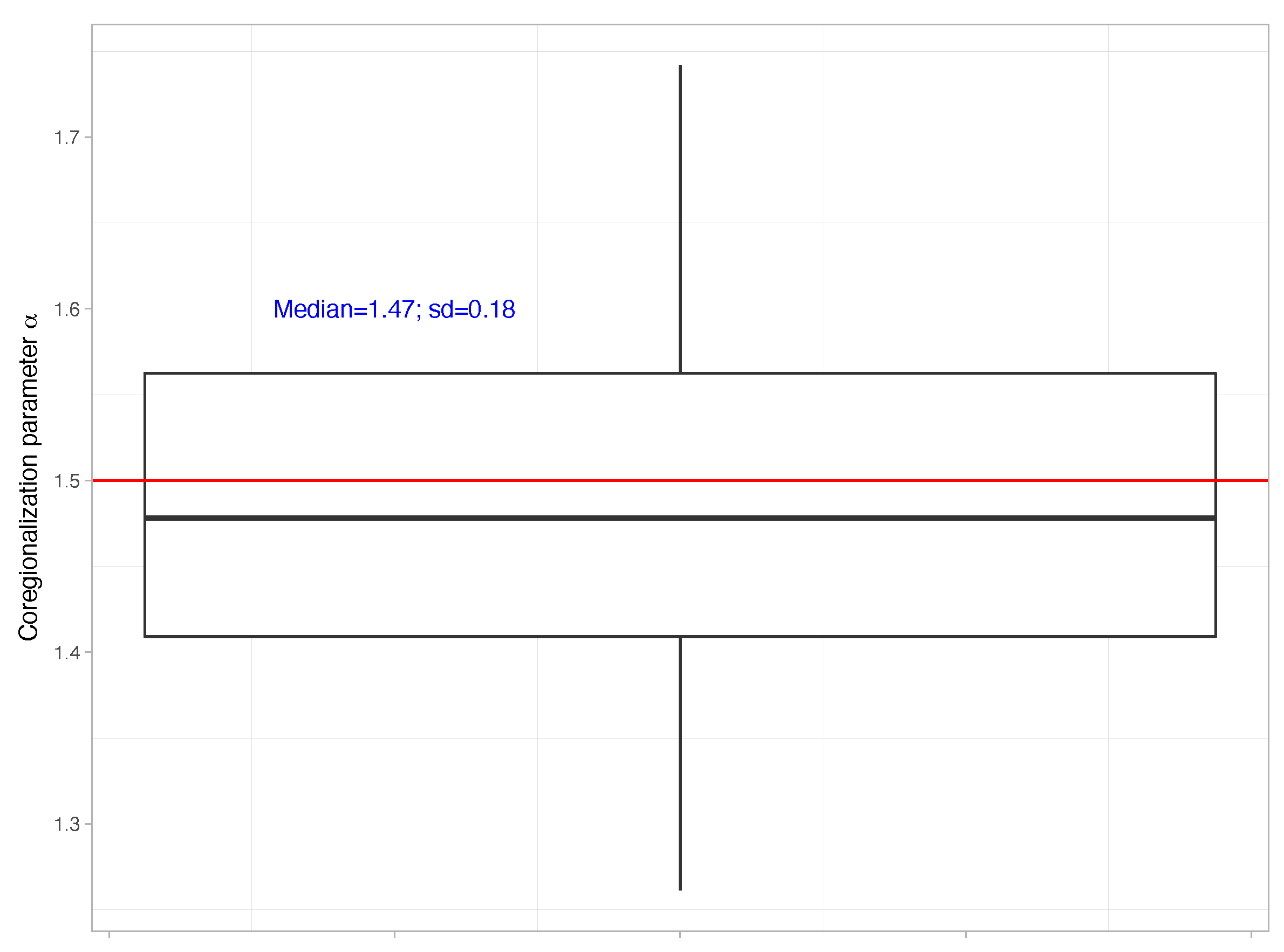
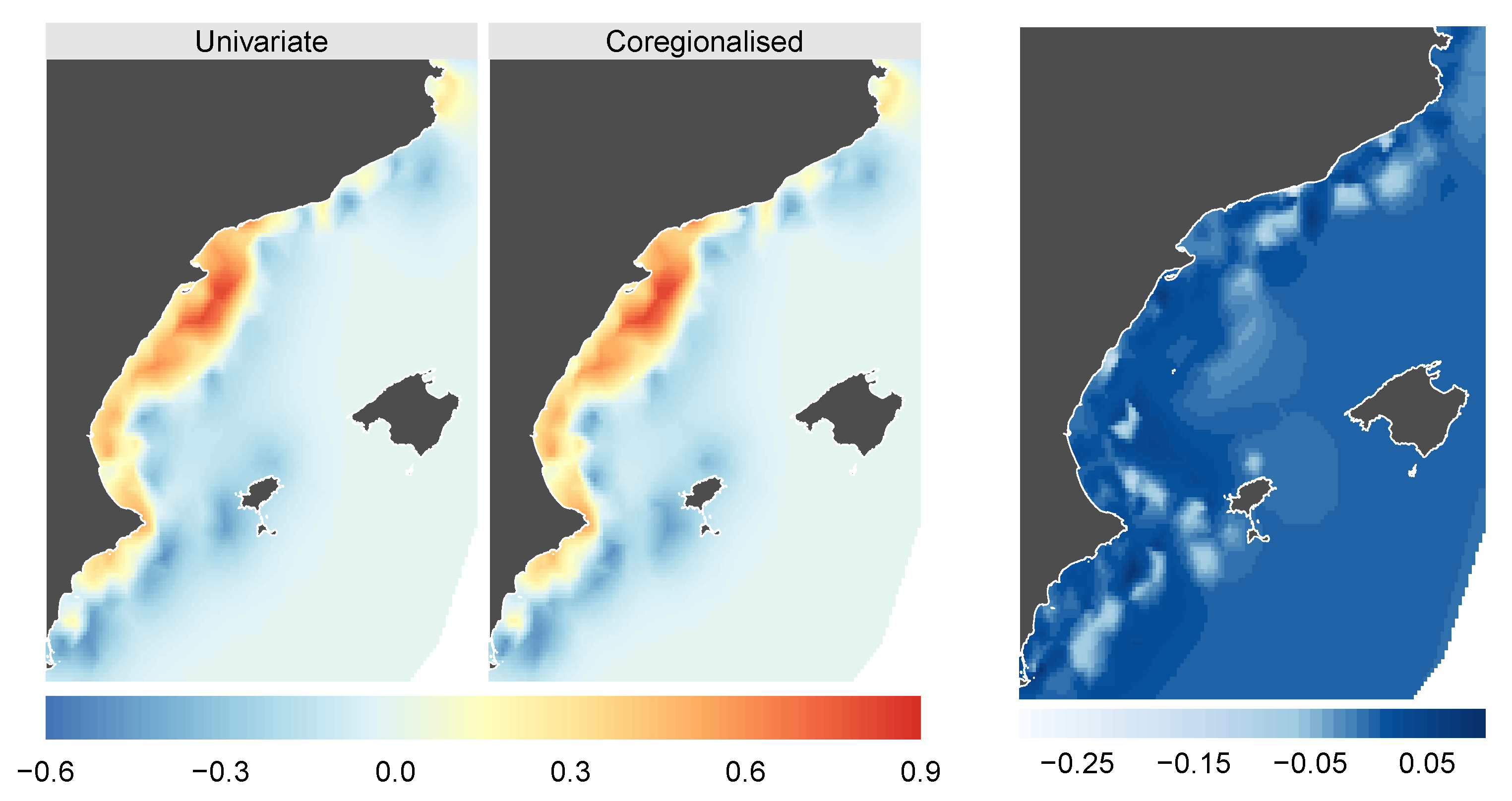
The coregionalized model that tries to reflect the relationship between the European anchovy and hake species is given by:
log ( Hake ) = β 10 + β 11 Bathymetry + W 1 + ϵ 1 log ( Anchovy ) = β 20 + β 21 Bathymetry + α W 1 + W 2 + ϵ 2
where log(Hake) and log(Anchovy) represent the logarithmic transformation of the mean biomass of both species in each sampling station. The linear predictors, which indicate how parameters behave in space, are formed by: β 10 and β 20 , i.e., the terms representing the intercepts of each variable; β 11 and β 21 , that represent the regression coefficients of a covariate introduced into the model, the bathymetry of the seabed for each sampling station; and W 1 and W 2 , that are the spatially structured effects. No interacting univariate models, i.e.,  α = 0 , were also implemented.
In order to facilitate the interpretation, we used a linear relationship between the fish species and the bathymetry variable, but a non-linear relationship could also have been fitted by incorporating second-order random walk latent models [41].
As no other information was available, we used non-informative Gaussian prior distributions with zero mean and standard deviation of 100 for all the fixed effects. PC-priors were used to describe prior knowledge of hyperparameters of the spatial terms. These priors were set as follows: if the prior probability of the spatial range was smaller than 0.1, it was set at 0.05, if the probability of the spatial variance was larger than 3, it was also set at 0.05.

4.3. Results

The coregionalized model in (11) and its corresponding univariate version were compared with submodels including fewer terms using a model fit measure, in particular WAIC [42]. All submodels resulted in a worse model fit.
Results of the inference process for the univariate and for the coregionalized model are summarised in Table 1 and Table 2, respectively. The association between European hake and anchovy is positive (i.e., mean α = 0.143), indicating that the geographical patterns of abundance of both species are related, and absorbs part of anchovies residual pattern (i.e., smaller σ 2 in the coregionalized model). This positive value is in line with [43], who concluded that predator–prey interactions may display positive or negative associations. The negative bathymetric effect was consistent across approaches, and suggests high abundances in shallow waters.
Figure 4 shows the mean of the spatial effect in the univariate (left map) and coregionalized models (middle map), as well as their difference (right map). As it can be seen, differences manifest in the transition zones between high and low abundances, providing a subtle improvement in the prediction of anchovy.
This improvement is also observed when analyzing the predictive capacity of both modelings through the predictive Mean Absolute Error (MAE) and Root Mean Square Error (RMSE) obtained for the univariate and coregionalized models (see Table 3). In particular, the model was fitted using data from 2000–2015, and the prediction was made for 2016 and compared with the observed values. Again, the coregionalized model shows lower values than the univariate model, both in terms of MAE and RMSE, indicating a better predictive capacity.

5. Concluding Remarks

There are still many issues to be tackled in species distribution modeling. Among them, this work has focused on the modeling of more than one species. We have revisited a spatial hierarchical Bayesian conditional coregionalized model to infer biotic associations in space. The main contribution has been to validate its behavior by means of a simulated example and a real application in the fisheries context.
Our results with simulated data indicate a better predictive capacity of the coregionalized approach. The coregionalized model successfully captured the association between species and the median MAE and RMSE scores were lower than those for the univariate model scores.
The practical application assessing the spatial distribution of prey, the European anchovy (Engraulis encrasicolus), and one of its predator species, European hake (Merluccius merluccius), in the Mediterranean sea has also shown a better behavior in the coregionalized model that includes biotic information. Main differences appear in the transition zones between high and low abundances, providing a subtle improvement in the prediction of anchovy. Moreover, the coregionalized model is better in terms of predictive capacity according to MAE and RMSE scores. Consequently, we conclude that this modeling could provide a better understanding of both species’ mesoscale ecology.
It is worth also noting that all this can be done thanks to the integrated nested Laplace approximation methodology and software that, jointly with the SPDE approach can help to minimize the computational burden while constituting a flexible tool in order to fit complex geostatistical models [44].
Finally, we would like to mention that this modeling could also include a temporal component that would allow us to analyze any possible temporal effect, in a similar way as in [23]. Moreover, it could also include other parametric or semiparametric constructions to reflect non-linear, autoregressive or more complex behaviors that would help to better describe the distribution of a species.

Author Contributions

Formal analysis, X.B., D.C., A.L.-Q., J.M.-M., I.P. and M.G.P.; Funding acquisition, D.C.; Investigation, X.B., D.C., A.L.-Q., J.M.-M., I.P. and M.G.P.; Methodology, X.B., D.C., A.L.-Q., J.M.-M., I.P. and M.G.P.; Writing—original draft, X.B., D.C., A.L.-Q., J.M.-M., I.P. and M.G.P.; Writing—review & editing, X.B., D.C., A.L.-Q., J.M.-M., I.P. and M.G.P. All authors have read and agreed to the published version of the manuscript.

Funding

X.B., D.C. and A.L.-Q. would like to thank the Spanish Ministerio de Ciencia e Innovación—Agencia Estatal de Investigación for grant PID2019-106341GB-I00 (jointly financed by the European Regional Development Fund, FEDER). M.G.P. also thanks the IMPRESS (RTI2018-099868-B-I00) project, ERDF, Ministry of Science, Innovation and Universities—State Research Agency. J.M.-M. thanks to the Basque Government BERC 2018–2021 program AEI-MCIU BCAM Severo Ochoa accreditation SEV-2017-0718. I.P. thanks the Marie Skłodowska-Curie grant agreement No 847014.

Institutional Review Board Statement

Not applicable.

Informed Consent Statement

Not applicable.

Data Availability Statement

Restrictions apply to the availability of these data. Data was obtained from Spanish Oceanographic Institute (IEO) and are available on request under the permission of IEO.

Acknowledgments

The authors express their gratitude to all the people that work in the MEDITS surveys and to everyone who has contributed to this study. Authors would also like to thank Lucía Martín for her careful reading of the manuscript and the English language revision.

Conflicts of Interest

The authors declare no conflict of interest.

References

  1. Guisan, A.; Thuiller, W. Predicting species distribution: Offering more than simple habitat models. Ecol. Lett. 2005, 8, 993–1009. [Google Scholar] [CrossRef]
  2. Elith, J.; Leathwick, J.R. Species distribution models: Ecological explanation and prediction across space and time. Annu. Rev. Ecol. Evol. Syst. 2009, 40, 677–697. [Google Scholar] [CrossRef]
  3. Fois, M.; Cuena-Lombraña, A.; Fenu, G.; Bacchetta, G. Using species distribution models at local scale to guide the search of poorly known species: Review, methodological issues and future directions. Ecol. Model. 2018, 385, 124–132. [Google Scholar] [CrossRef] [Green Version]
  4. Martínez-Minaya, J.; Cameletti, M.; Conesa, D.; Pennino, M.G. Species distribution modeling: A statistical review with focus in spatio-temporal issues. Stoch. Environ. Res. Risk Assess. 2018, 32, 3227–3244. [Google Scholar] [CrossRef]
  5. Coll, M.; Pennino, M.G.; Steenbeek, J.; Solé, J.; Bellido, J.M. Predicting marine species distributions: Complementarity of food-web and Bayesian hierarchical modelling approaches. Ecol. Model. 2019, 405, 86–101. [Google Scholar] [CrossRef]
  6. Pearson, R.G.; Dawson, T. Predicting the impacts of climate change on the distribution of species: Are bioclimate envelope models useful? Glob. Ecol. Biogeogr. 2003, 12, 361–371. [Google Scholar] [CrossRef] [Green Version]
  7. Wisz, M.S.; Pottier, J.; Kissling, W.D.; Pellissier, L.; Lenoir, J.; Damgaard, C.F.; Dormann, C.F.; Forchhammer, M.C.; Grytnes, J.A.; Guisan, A.; et al. The role of biotic interactions in shaping distributions and realised assemblages of species: Implications for species distribution modelling. Biol. Rev. 2013, 88, 15–30. [Google Scholar] [CrossRef] [Green Version]
  8. Sánchez-Cordero, V.; Martínez-Meyer, E. Museum specimen data predict crop damage by tropical rodents. Proc. Natl. Acad. Sci. USA 2000, 97, 7074–7077. [Google Scholar] [CrossRef] [PubMed]
  9. Hebblewhite, M.; Merrill, E.; McDonald, T. Spatial decomposition of predation risk using resource selection functions: An example in a wolf-elk predator-prey system. Oikos 2005, 111, 101–111. [Google Scholar] [CrossRef]
  10. Trainor, A.M.; Schmitz, O.J.; Ivan, J.S.; Shenk, T.M. Enhancing species distribution modeling by characterizing predator–prey interactions. Ecol. Appl. 2014, 24, 204–216. [Google Scholar] [CrossRef]
  11. Peterson, A.; Sánchez-Cordero, V.; Beard, C.; Ramsey, J. Ecologic niche modeling and potential reservoirs for Chagas disease, Mexico. Emerg. Infect. Dis. 2002, 8, 662–667. [Google Scholar] [CrossRef]
  12. Giannini, T.C.; Chapman, D.S.; Saraiva, A.M.; Alves-dos Santos, I.; Biesmeijer, J.C. Improving species distribution models using biotic interactions: A case study of parasites, pollinators and plants. Ecography 2013, 36, 649–656. [Google Scholar] [CrossRef] [Green Version]
  13. Gutiérrez, D.; Fernández, P.; Seymour, A.; Jordano, D. Habitat distribution models: Are mutualist distributions good predictors of their associates? Ecol. Appl. 2005, 15, 3–18. [Google Scholar] [CrossRef]
  14. Vasconcelos, T.S.; Antonelli, C.P.; Napoli, M.F. Mutualism influences species distribution predictions for a bromeliad-breeding anuran under climate change. Austral Ecol. 2017, 42, 869–877. [Google Scholar] [CrossRef]
  15. Aarts, G.; Jones, E.; Brasseur, S.; Rindorf, A.; Smout, S.; Dickey-Collas, M.; Wright, P.; Russell, D.; McConnell, B.; Kirkwood, R.; et al. Prey habitat model outperforms prey data in explaining grey seal distribution. In Proceedings of the Annual Conferenec of the European Cetacean Society, La Rochelle, France, 5–9 April 2014. [Google Scholar]
  16. Pennino, M.G.; Guijarro-García, E.; Vilela, R.; del Río, J.L.; Bellido, J.M. Modeling the distribution of thorny skate (Amblyraja radiata) in the southern Grand Banks (Newfoundland, Canada). Can. J. Fish. Aquat. Sci. 2019, 76, 2121–2130. [Google Scholar] [CrossRef]
  17. Chiles, J.; Delfiner, P. Geoestatistics: Modeling Spatial Uncertainty; Wiley: New York, NY, USA, 1999. [Google Scholar]
  18. Wackernagel, H. Multivariate Geostatistics: An Introduction with Applications, 3rd ed.; Springer: New York, NY, USA, 2003. [Google Scholar]
  19. Gelfand, A.; Diggle, P.; Guttorp, P.; Fuentes, M. Handbook of Spatial Statistics; CRC Press: Boca Raton, FL, USA, 2010. [Google Scholar]
  20. Banerjee, S.; Carlin, B.; Gelfand, A. Hierarchical Modeling and Analysis for Spatial Data, 2nd ed.; Chapman and Hall/CRC: Boca Raton, FL, USA, 2014. [Google Scholar]
  21. Gelfand, A.E.; Banerjee, S. Bayesian Modeling and Analysis of Geostatistical Data. Annu. Rev. Stat. Appl. 2017, 4, 245–266. [Google Scholar] [CrossRef] [Green Version]
  22. Schmidt, A.M.; Gelfand, A.E. A Bayesian coregionalization approach for multivariate pollutant data. J. Geophys. Res. Atmos. 2003, 108, 8783. [Google Scholar] [CrossRef]
  23. Jones-Todd, C.M.; Swallow, B.; Illian, J.B.; Toms, M. A spatiotemporal multispecies model of a semicontinuous response. J. R. Stat. Soc. Ser. C Appl. Stat. 2018, 67, 705–722. [Google Scholar] [CrossRef]
  24. Barber, X.; Conesa, D.; López-Quílez, A.; Morales, J. Multivariate Bioclimatic Indices Modelling: A Coregionalised Approach. J. Agric. Biol. Environ. Stat. 2019, 24, 225–244. [Google Scholar] [CrossRef]
  25. Rue, H.; Martino, S.; Chopin, N. Approximate Bayesian inference for latent Gaussian models by using integrated nested Laplace approximations. J. R. Stat. Soc. Ser. B Stat. Methodol. 2009, 71, 319–392. [Google Scholar] [CrossRef]
  26. Gilks, W.; Richardson, S.; Spiegelhalter, D. Markov Chain Monte Carlo in Practice; Chapman and Hall/CRC: Boca Raton, FL, USA, 1996. [Google Scholar]
  27. Barber, X.; Conesa, D.; López-Quílez, A.; Mayoral, A.; Morales, J.; Barber, A. Bayesian hierarchical models for analysing the spatial distribution of bioclimatic indices. SORT-Stat. Oper. Res. Trans. 2017, 1, 277–296. [Google Scholar]
  28. Genton, M.G.; Kleiber, W. Cross-covariance functions for multivariate geostatistics. Stat. Sci. 2015, 30, 147–163. [Google Scholar] [CrossRef]
  29. Cressie, N.; Zammit-Mangion, A. Multivariate spatial covariance models: A conditional approach. Biometrika 2016, 103, 915–935. [Google Scholar] [CrossRef]
  30. Gelfand, A. Hierarchical modeling for spatial data problems. Spat. Stat. 2012, 1, 30–39. [Google Scholar] [CrossRef] [Green Version]
  31. Matérn, B. Spatial Variation, 2nd ed.; Springer: Berlin, Germany, 1986. [Google Scholar]
  32. Abramowitz, M.; Stegun, I. Handbook of Mathematical Functions: With Formulas, Graphs, and Mathematical Tables; National Bureau of Standards: Washington, DC, USA, 1964. [Google Scholar]
  33. Lindgren, F.; Rue, H.; Lindström, J. An explicit link between Gaussian fields 670 and Gaussian Markov random fields: The SPDE approach (with discussion). J. R. Stat. Soc. Ser. B 2011, 73, 423–498. [Google Scholar] [CrossRef] [Green Version]
  34. Krainski, E.; Gómez-Rubio, V.; Bakka, H.; Lenzi, A.; Castro-Camilo, D.; Simpson, D.; Lindgren, F.; Rue, H. Advanced Spatial Modeling with Stochastic Partial Differential Equations Using R and INLA; Chapman and Hall/CRC: Boca Raton, FL, USA, 2019. [Google Scholar]
  35. Rue, H.; Riebler, A.; Sørbye, S.; Illian, J.; Simpson, D.; Lindgren, F. Bayesian computing with INLA: A review. Annu. Rev. Stat. Appl. 2017, 4, 395–421. [Google Scholar] [CrossRef] [Green Version]
  36. Blangiardo, M.; Cameletti, M. Spatial and Spatio-Temporal Bayesian Models with R-INLA; John Wiley & Sons: New York, NY, USA, 2015. [Google Scholar]
  37. Fuglstad, G.A.; Simpson, D.; Lindgren, F.; Rue, H. Constructing priors that penalize the complexity of Gaussian random fields. J. Am. Stat. Assoc. 2019, 114, 445–452. [Google Scholar] [CrossRef] [Green Version]
  38. Simpson, D.; Rue, H.; Riebler, A.; Martins, T.G.; Sørbye, S.H. Penalising model component complexity: A principled, practical approach to constructing priors. Stat. Sci. 2017, 32, 1–28. [Google Scholar] [CrossRef]
  39. Schlather, M.; Malinowski, A.; Menck, P.J.; Oesting, M.; Strokorb, K. Analysis, simulation and prediction of multivariate random fields with package RandomFields. J. Stat. Softw. 2015, 63, 1–25. [Google Scholar] [CrossRef] [Green Version]
  40. Bertrand, J.A.; de Sola, L.G.; Papaconstantinou, C.; Relini, G.; Souplet, A. The general specifications of the MEDITS surveys. Sci. Mar. 2002, 66, 9–17. [Google Scholar] [CrossRef] [Green Version]
  41. Fahrmeir, L.; Lang, S. Bayesian semiparametric regression analysis of multicategorical time-space data. Ann. Inst. Stat. Math. 2001, 53, 11–30. [Google Scholar] [CrossRef]
  42. Watanabe, S. Asymptotic equivalence of Bayes cross validation and widely applicable information criterion in singular learning theory. J. Mach. Learn. Res. 2010, 11, 3571–3594. [Google Scholar]
  43. Zurell, D.; Pollock, L.; Thuiller, W. GDo joint species distribution models reliably detect interspecific interactions from co-occurrence data in homogenous environments? Ecogr. Model. 2018, 41, 1812–1819. [Google Scholar] [CrossRef] [Green Version]
  44. Pennino, M.G.; Paradinas, I.; Illian, J.B.; Muñoz, F.; Bellido, J.M.; López-Quílez, A.; Conesa, D. Accounting for preferential sampling in species distribution models. Ecol. Evol. 2019, 9, 653–663. [Google Scholar] [CrossRef]
Figure 1. Boxplot of the posterior means of the parameter α obtained by fitting each of the 40 simulated realisations.
Mathematics 09 00417 g001
Figure 2. MAE and RMSE for the univariate and coregionalized model using the test samples (40% of the simulated data).
Mathematics 09 00417 g002
Figure 3. Map of the study area showing the abundance at each of the annual sampling locations and basic statistics (mean and standard deviation) for both the European anchovy (Engraulis encrasicolus, left) and the European hake (Merluccius merluccius, right).
Mathematics 09 00417 g003
Figure 4. Maps of posterior mean of the spatial effect in the univariate model (left), the coregionalized model (middle), and the difference of the two spatial effects (right) for the European anchovy (Engraulis encrasicolus).
Mathematics 09 00417 g004
Table 1. Point estimates (mean, median and standard deviation) along with 95% credible interval of the posterior distribution of the fixed effects and the hyperparameters of the univariate models for both the European anchovy (Engraulis encrasicolus) and the European hake (Merluccius merluccius).
Meansd q 0.025 q 0.5 q 0.975
Hake
β 10 6.56340.27116.00596.57277.0698
β 11 −0.00390.0007−0.0053−0.0039−0.0025
ϕ 1 0.1540.0270.1070.1520.214
σ 1 2.1470.1541.8632.1412.466
Anchovies
β 20 4.47560.41603.588314.49725.2391
β 21 −0.00250.0007−0.0039−0.0025−0.0010
ϕ 2 0.6140.1660.3710.5851.015
σ 2 1.6230.2201.2511.6022.113
Table 2. Point estimates (mean, median and standard deviation) along with 95% credible interval of the posterior distribution of the fixed effects and the hyperparameters of the coregionalized approach for both the European anchovy (Engraulis encrasicolus) and the European hake (Merluccius merluccius).
Meansd q 0.025 q 0.5 q 0.975
β 10 6.52580.27595.96006.53437.0434
β 20 4.44260.39343.60914.46095.1692
β 11 −0.00380.0007−0.0052−0.0038−0.0024
β 21 −0.00210.0008−0.0036−0.0021−0.0006
ϕ 1 0.1610.0280.1130.1580.223
σ 1 2.1480.1521.8642.1432.463
ϕ 2 0.5750.1540.3500.5480.948
σ 2 1.5440.1941.2121.5271.971
α 0.1430.073−0.0030.1440.285
Table 3. Predictive capacity of Univariate and coregionalized models obtained by cross-validation of real 2016 data with the previous adjusted model.
ModelMeasureValue
UnivariateMAE4212.35
CoregionalisationMAE3842.35
UnivariateRMSE8422.54
CoregionalisationRMSE7697.88
Publisher’s Note: MDPI stays neutral with regard to jurisdictional claims in published maps and institutional affiliations.

