Robust Sensorless Model-Predictive Torque Flux Control for High-Performance Induction Motor Drives

Abstract

This paper introduces a novel sensorless model-predictive torque-flux control (MPTFC) for two-level inverter-fed induction motor (IM) drives to overcome the high torque ripples issue, which is evidently presented in model-predictive torque control (MPTC). The suggested control approach will be based on a novel modification for the adaptive full-order-observer (AFOO). Moreover, the motor is modeled considering core losses and a compensation term of core loss applied to the suggested observer. In order to mitigate the machine losses, particularly at low speed and light load operations, the loss minimization criterion (LMC) is suggested. A comprehensive comparative analysis between the performance of IM drive under conventional MPTC, and those of the proposed MPTFC approaches (without and with consideration of the LMC) has been carried out to confirm the efficiency of the proposed MPTFC drive. Based on MATLAB^® and Simulink^® from MathWorks^® (2018a, Natick, MA 01760-2098 USA) simulation results, the suggested sensorless system can operate at very low speeds and has the better dynamic and steady-state performance. Moreover, a comparison in detail of MPTC and the proposed MPTFC techniques regarding torque, current, and fluxes ripples is performed. The stability of the modified adaptive closed-loop observer for speed, flux and parameters estimation methodology is proven for a wide range of speeds via Lyapunov’s theorem.

1. Introduction

Several schemes for speed-sensorless vector-controlled induction motor (IM) drives have been suggested for nearly a decade. Via flux and speed sensors positioned within the machine will deteriorate the machine’s robustness and raise the associated maintenance expenses. Speed sensor cost is within the same range as the price of motor itself, at least for machines with ratings below$10\mathrm{kW}$. In many applications, sensor mounting to the motor is an obstacle. The majority of estimators proposed in sensorless IM drives for combined flux and also speed estimation could be divided into three categories: (a) Model-reference-adaptive system (MRAS) [1,2]. Although MRAS-based estimators are favored due to simplicity, ease of implementation, and documented stability [3], they have certain drawbacks in the low-speed zone, where open-loop integration can result in instability due to stator resistance misestimating [4]. (b) Full-order observers (FOO) [5] providing both stator current and stator or rotor flux estimates. In FOO, alteration is made throughout the error between both measured stator current and its estimated value that is often used to adjust estimated speed in an adaptation law. (c) Reduced-order observers (ROO) [6], that are only rotor or stator flux estimators. It is the potential to make the ROO essentially sensorless [7], i.e., speed will not appear in the observer equations. The major drawback for sensorless velocity drives is their poor performance when IM operates at lowish velocity range or near zero-velocity point. However, low-velocity and zero-velocity operating case of IMs is the popular for industrial applications, like hoists (sometimes operating at $0.5\mathrm{Hz}$ to $1\mathrm{Hz}$), marble cutting machines (operating at $0.3\mathrm{Hz}$ sometimes) and mine carrier cars (sometimes operating at$0\mathrm{Hz}$). Therefore, sensorless drives performance at low-velocity ranges necessities to be improved.

To achieve an active decoupled control for flux and electromagnetic torque, the direct torque control (DTC) was offered to replace the field-oriented control (FOC) in the drive domain. DTC provides a simpler scheme, faster response, and lower machine parameter dependency than FOC. Besides that, it does not include coordinates transformation or current regulations [8,9]. The key problem of this technique is the excessive amount of flux and also electromagnetic torque ripples created through the variable switching frequency due to discrete nature of the hysteresis comparators and voltage vector selection look-up-table (LUT) [10].

In order to address some weaknesses in classical DTC techniques, an effective control approach called model predictive control (MPC), has recently been proposed. MPC’s key advantages are its ability to recognize various control targets, the straightforward management of nonlinearities and control limits of the model, and easy implementation [11,12,13,14]. Recent works have implemented MPC method to avoid limitations of classical LUT-based DTC of IM drives [15,16,17,18]. The proposed MPDTC techniques implemented in these studies contributed to improving the drive’s dynamic efficiency, but as an essential feature of the regulated variables, the ripple content was still present. There are different explanations for why the ripple phenomena in the MPDTC are presented. The foremost one would be originated in view of the technique principle of MPDTC itself. After the minimization of a cost function, it selects a voltage vector and inevitably applies this vector for the entire subsequent sampling duration, even though this is deleterious in certain situations, as it may occur that the regulated quantity (i.e., the torque) is therefore pushed out of reasonable limits before the end of the loop.

Different methods have been established to eliminate unwanted ripples, such as splitting the sampling interval into two parts and adding dual different voltage vectors in each interval [19,20,21], for example. This has essentially helped to limit the ripples. Otherwise, the complexities and computational burden of those methods are amplified and this would affect the dynamic digital control response, which is intended to be very rapid in many numbers of industrial applications.

Model-predictive current control (MPCC) was presented in [22,23] as a solution to limit the use of the cost function weighting value. Two prediction horizons were suggested in [23] to predict stator currents, which resulted in the reduction of the accompanying noise. However, measurement time was increased, otherwise amplifying the commutations of the inverter.

Due to its intuitive definition, high versatility, and simple incorporation of constraints, model-predictive torque control (MPTC) has recently gained significant attention within the academic and industrial communities [24,25]. Despite the MPTC’s intuitive definition and rapid response, as stator flux and also torque control variables have different amplitudes and units, a proper stator flux weighting factor should be built to achieve adequate performance [13,26,27].

Model-predictive flux control (MPFC) is suggested in [28] and compared with the conventional MPTC in [29] to prevent nontrivial weighting factor adjustment effort for MPTC. While in [13], the prediction errors are translated into ranking values for different control variables. As the finest one, the voltage vector leading to the minimum average ranking value is chosen.

Model-Predictive torque and flux control (MPTFC) [30] for variable speed drives is a significant member of the finite control set model-predictive control (FCS-MPC) family. A significant level of robustness to model parameter deviations could be achieved by directly controlling machine magnetization and electromagnetic torque [31]. Throughout the cost function, the expected errors of torque and stator flux magnitude are enhanced. A corresponding objective function, subject to inverter and machine model, is minimized online to this end. This results in an optimum switch position (i.e., control input) applied to the power converter [32].

Another feature of IM drives is that they exhibit greater efficiency when working at rated load [33,34]. However, owing to the persistence of iron losses and a part of copper losses, efficiency deteriorates under light load operation. This factor would harm the machine service life; accordingly, a criterion should be adopted to mitigate losses, particularly at light loads. Techniques for efficiency optimization are typically categorized into two types: search methods and model-based methods centered on how to decide the steady-state-optimal control variable [35]. Search-based methods are techniques of perturbation and observation that push the control command in the direction of minimal power losses. If closed-form solutions are not available, machine losses could either be calculated via loss model or measured using a power analyzer. Search-based strategies still struggle from a slow convergence rate and undesirable torque dynamics and fluctuations [36], despite attempts to raise the convergence rate using mathematical algorithms.

As a consequence, approaches focused on search are limited to steady-state processes. Multiple flux modes exist for industrial applications. The control minimizing loss is only switched on at steady-state, and during transients, the rated flux is usually linked to fast torque dynamics. There is no clear identification of transitions between flux modes during torque transients [37]. When the stator flux linkage shifts rapidly during torque transients, major losses are caused. Consequently, for highly dynamic load profiles, the steady-state optimal solution causes even more losses than constant rated flux operation.

An adaptive observer for combined flux and speed guesstimate in rotor speed reference frame is suggested in this paper. Rather than the traditional rotor flux plus stator current IM model, the rotor and stator flux models are utilized in the rotor speed reference frame. This makes it probable to apply the suggested observer in both stator and rotor-flux vector-controlled IM drives and in DTC-IM drives. It should also be mentioned that both stator and rotor resistance values and estimated velocity are the uncertainties considered in this article.

The current study introduces an efficient MPTFC technique for the IM drive in which some of the MPTC shortcomings can be mitigated, in specific by reducing the ripples of torque, stator flux and current. Furthermore, a loss minimization criterion (LMC) is suggested to improve the drive efficiency, particularly under light loads and low-speed operations, extending the IM’s lifetime. Drive efficiency is validated by comprehensive simulation testing, in which the feasibility of the MPTFC strategy is demonstrated. The combination of prediction and estimation, in this work, is the additional challenge of sensorless MPTFC approach versus traditional sensorless approaches. The paper’s contributions could be summarized as follows; the work intends to eliminate and replace the mechanical sensor with novel soft sensorless algorithms to minimize the drive cost and boost its reliability. Moreover, the paper offers a novel predictive torque-flux control approach for IM drive. Representing the IM model with consideration of core-loss and illustration of the used $2-$level voltage source inverter has been implemented. Developing a novel AFOO, which contributes to reducing the fluctuations and thereby enhancing the method torque-flux and prediction, with the compensation of core-loss, for; rotor speed estimation, stator flux estimation, rotor flux estimation, stator and rotor resistance estimation, stator current estimation, electromagnetic torque estimation has been introduced. The analysis and design of the proposed MPTFC strategy are described in a straightforward manner that clarifies the suggested drive basic operation. To minimalize the copper and iron losses, particularly at low-velocity and light loading, which enhances the IM efficiency, an LMC is provided in steady-state operation. In order to assess IM dynamics under the proposed MPTFC and MPTC approaches, comprehensive simulation tests are conducted. Test results approve the suggested MPTFC reliability to be used as a stronger alternative to the MPTC. All gain selections of controllers and controllers that have been designed to ensure overall drive stability shall be found in Appendix A.

The paper starts with the implementation of the IM mathematical model and $2-$level inverter, with consideration of core-loss. Then, the proposed AFOO is designed and explained. The suggested MPTFC method is subsequently presented and explained in-depth, and the proposed LCM is then presented and systematically evaluated. Eventually, the complete system design and performance test results are introduced and discussed.

2. Mathematical Model of IM and Inverter

In the stationary ($\mathsf{\alpha }-\mathsf{\beta }$) reference frame, indicated by the apex $\mathrm{s}$ for the stator and rotor amounts, Figure 1 demonstrates the IM model. No transformation of stator amounts (indicated by index$\mathrm{s}$) is necessary for this frame, while the rotor amount (index$\mathrm{rs}$) simply refers to the stator. Even though all of them remain sinusoidal during steady-state activity, this model makes it easier to formulate the predictive torque and flux control model proposed. Stator and rotor voltage balance equations in Figure 1 are provided as in (1) and (2) in the continuous time domain [38,39]:

$$\mathrm{p}{\overrightarrow{\mathrm{\Psi }}}_{\mathrm{s}}={\overrightarrow{\mathrm{v}}}_{\mathrm{s}}-{\mathrm{R}}_{\mathrm{s}}{\overrightarrow{\mathrm{i}}}_{\mathrm{s}}$$

(1)

$$\mathrm{p}{\overrightarrow{\mathrm{\Psi }}}_{\mathrm{rs}}=-{\mathrm{R}}_{\mathrm{r}}^{\text{′}}{\overrightarrow{\mathrm{i}}}_{\mathrm{rs}}+{\mathrm{j}\mathsf{\omega }}_{\mathrm{me}}{\overrightarrow{\mathrm{\Psi }}}_{\mathrm{rs}}$$

(2)

where $\mathrm{p}$ is a differential operator,${\mathsf{\omega }}_{\mathrm{me}}={\mathrm{P}\mathsf{\omega }}_{\mathrm{m}}$, with $\mathrm{P}$ is pole pairs and ${\mathsf{\omega }}_{\mathrm{m}}$ is the shaft speed. Additionally,${\mathrm{L}}_{\mathsf{\sigma }\mathrm{s}}$and ${\mathrm{R}}_{\mathrm{s}}$ are stator leakage inductance and resistance, respectively; ${\mathrm{L}}_{\mathsf{\sigma }\mathrm{r}}^{\text{′}}$ and ${\mathrm{R}}_{\mathrm{r}}^{\text{′}}$ are rotor leakage inductance and resistance, respectively, both referred to the stator; and ${\mathrm{R}}_{\mathrm{fe}}$, ${\mathrm{L}}_{\mathrm{m}}$ are the equivalent resistance representing the iron losses, and the magnetizing inductance, respectively. The relationships among currents and fluxes and are assumed linear (no saturation) and are listed as follows:

$${\overrightarrow{\mathrm{\Psi }}}_{\mathrm{s}}={\mathrm{L}}_{\mathsf{\sigma }\mathrm{s}}{\overrightarrow{\mathrm{i}}}_{\mathrm{s}}+{\mathrm{L}}_{\mathrm{m}}{\overrightarrow{\mathrm{i}}}_{\mathrm{m}}={\mathrm{L}}_{\mathsf{\sigma }\mathrm{s}}{\overrightarrow{\mathrm{i}}}_{\mathrm{s}}+{\overrightarrow{\mathrm{\Psi }}}_{\mathrm{m}}$$

(3)

$${\overrightarrow{\mathrm{\Psi }}}_{\mathrm{rs}}={\mathrm{L}}_{\mathsf{\sigma }\mathrm{r}}^{\text{′}}{\overrightarrow{\mathrm{i}}}_{\mathrm{rs}}+{\mathrm{L}}_{\mathrm{m}}{\overrightarrow{\mathrm{i}}}_{\mathrm{m}}={\mathrm{L}}_{\mathsf{\sigma }\mathrm{r}}^{\text{′}}{\overrightarrow{\mathrm{i}}}_{\mathrm{rs}}+{\overrightarrow{\mathrm{\Psi }}}_{\mathrm{m}}$$

(4)

where ${\overrightarrow{\mathrm{\Psi }}}_{\mathrm{m}}$ and ${\overrightarrow{\mathrm{i}}}_{\mathrm{m}}$ are magnetizing air-gap flux and magnetizing current, respectively. Furthermore,

$${\mathrm{R}}_{\mathrm{fe}}{\overrightarrow{\mathrm{i}}}_{\mathrm{fe}}={\mathrm{L}}_{\mathrm{m}}\mathrm{p}{\overrightarrow{\mathrm{i}}}_{\mathrm{m}}$$

(5)

$${\overrightarrow{\mathrm{i}}}_{\mathrm{m}}+{\overrightarrow{\mathrm{i}}}_{\mathrm{fe}}={\overrightarrow{\mathrm{i}}}_{\mathrm{s}}+{\overrightarrow{\mathrm{i}}}_{\mathrm{rs}}$$

(6)

With some management of the equations, Equation (2) can be replaced by

$$\mathrm{p}{\overrightarrow{\mathrm{i}}}_{\mathrm{s}}=\frac{{\mathrm{L}}_{\mathrm{m}}}{{\mathrm{L}}_{\mathrm{m}}{\mathrm{L}}_{\mathsf{\sigma }\mathrm{r}}^{\text{′}}+{\mathrm{L}}_{\mathsf{\sigma }\mathrm{s}}\left({\mathrm{L}}_{\mathsf{\sigma }\mathrm{r}}^{\text{′}}+{\mathrm{L}}_{\mathrm{m}}\right)}\left\{\left(\frac{{\mathrm{L}}_{\mathsf{\sigma }\mathrm{r}}^{\text{′}}+{\mathrm{L}}_{\mathrm{m}}}{{\mathrm{L}}_{\mathrm{m}}}\right){\overrightarrow{\mathrm{v}}}_{\mathrm{s}}-\left[{\mathrm{R}}_{\mathrm{s}}\left(\frac{{\mathrm{L}}_{\mathsf{\sigma }\mathrm{r}}^{\left\{\text{′}\right\}}+{\mathrm{L}}_{\mathrm{m}}}{{\mathrm{L}}_{\mathrm{m}}}\right)+{\mathrm{R}}_{\mathrm{r}}^{\text{′}}\right]{\overrightarrow{\mathrm{i}}}_{\mathrm{s}}+{\mathrm{R}}_{\mathrm{r}}^{\text{′}}\left({\overrightarrow{\mathrm{i}}}_{\mathrm{m}}+{\overrightarrow{\mathrm{i}}}_{\mathrm{fe}}\right)-{\mathrm{j}\mathsf{\omega }}_{\mathrm{me}}{\overrightarrow{\mathrm{i}}}_{\mathrm{r}}\right\}$$

(7)

Although dynamic IM performance is well represented in Equations (1) and (7), it is very multifaceted to appreciate. We suppose to rewrite the following Equations (8)–(11) to characterize the IM state-space model in terms of equivalent core-loss resistance,${\mathrm{R}}_{\mathrm{m}}$, which is included in ${\mathrm{R}}_{\mathrm{fe}}$ where ${\mathrm{R}}_{\mathrm{m}}$ is presumed to be proportional to ${\mathsf{\omega }}^{1.6 }$ [40].

$$p{i}_{\alpha s}=-\left(\frac{R_s}{L_s \sigma }+\frac{R_r L_m^2}{L_s L_r^2 \sigma }\right)i_{\alpha s}+\left[\frac{R_r L_m+R_m\left(s{L}_m-L_r\right)}{L_s L_r^2 \sigma }\right]{\Psi }_{\alpha r}+\frac{L_m}{L_s L_r \sigma }{\omega }_r{\Psi }_{\beta r}+\frac{1}{L_s \sigma }{v}_{\alpha s}$$

(8)

$$p{i}_{\beta s}=-\left(\frac{R_s}{L_s \sigma }+\frac{R_r L_m^2}{L_s{L}_r^2\sigma }\right)i_{\mathsf{\beta }s}+\left[\frac{R_r L_m+R_m\left(s{L}_m-L_r\right)}{L_s L_r^2 \sigma }\right]{\Psi }_{\mathsf{\beta }r}-\frac{L_m}{L_s L_r \sigma }{\omega }_r{\Psi }_{\alpha r}+\frac{1}{L_s\sigma }{v}_{\beta s}$$

(9)

$${\mathrm{p}\mathrm{\Psi }}_{\mathsf{\alpha }\mathrm{r}}=\frac{{\mathrm{R}}_{\mathrm{r}}{\mathrm{L}}_{\mathrm{m}}}{{\mathrm{L}}_{\mathrm{r}}} {\mathrm{i}}_{\mathsf{\alpha }\mathrm{s}}-\left(\frac{{\mathrm{R}}_{\mathrm{r}}-\mathrm{s}}{{\mathrm{L}}_{\mathrm{r}}}\right){\mathrm{\Psi }}_{\mathsf{\alpha }\mathrm{r}}-{\mathsf{\omega }}_{\mathrm{r}}{\mathrm{\Psi }}_{\mathsf{\beta }\mathrm{r}}$$

(10)

$${\mathrm{p}\mathrm{\Psi }}_{\mathsf{\beta }\mathrm{r}}=\frac{{\mathrm{R}}_{\mathrm{r}} {\mathrm{L}}_{\mathrm{m}}}{{\mathrm{L}}_{\mathrm{r}}} {\mathrm{i}}_{\mathsf{\beta }\mathrm{s}}-\left(\frac{{\mathrm{R}}_{\mathrm{r}}-\mathrm{s}}{{\mathrm{L}}_{\mathrm{r}}}\right){\mathrm{\Psi }}_{\mathsf{\beta }\mathrm{r}}+{\mathsf{\omega }}_{\mathrm{r}}{\mathrm{\Psi }}_{\mathsf{\alpha }\mathrm{r}}$$

(11)

where${\mathsf{\omega }}_{\mathrm{r}}$ is the rotor speed, $\mathrm{s}$ is the slip and $\mathsf{\omega }$ is the excitation frequency. Cross product of rotor and stator flux linkages vectors states the developed torque [28] as:

$${\mathrm{T}}_{\mathrm{e}}=\frac{3}{2}\mathrm{P}\frac{{\mathrm{L}}_{\mathrm{m}}}{{\mathrm{L}}_{\mathrm{r}}{\mathrm{L}}_{\mathrm{s}}-{\mathrm{L}}_{\mathrm{m}}{}^2}\left({\overrightarrow{\mathrm{\Psi }}}_{\mathrm{s}}\times {\overrightarrow{\mathrm{\Psi }}}_{\mathrm{r}}\right)$$

(12)

For both MPTC and MPTFC methods, a $2-$level voltage source inverter (VSI) is used in this work. The inverter topology and its feasible voltage vectors are shown in Figure 2. With every phase$\mathrm{A}$, $\mathrm{B}$ and $\mathrm{C}$the responding switching state $\mathrm{S}$ can be described as:

$$\mathrm{S}=\frac{2}{3}\left({\mathrm{S}}_{\mathrm{a}}+{\mathrm{a}\mathrm{S}}_{\mathrm{b}}+{\mathrm{a}}^2{\mathrm{S}}_{\mathrm{c}}\right)$$

(13)

where $\mathrm{A}$,$\mathrm{B}$ and $\mathrm{C}$ are motor terminals, $\mathrm{a}={\mathrm{e}}^{\mathrm{j}2\mathsf{\pi }/3}$, ${\mathrm{S}}_{\mathrm{i}}=1$ means ${\mathrm{S}}_{\mathrm{i}}$ on, ${\overline{\mathrm{S}}}_{\mathrm{i}}$ means off and DC-bus voltage is ${\mathrm{V}}_{\mathrm{dc}}$.

The relation between inverter output voltage vector ${\overrightarrow{\mathrm{v}}}_{\mathrm{s}\mathsf{\alpha }\mathsf{\beta },\mathrm{k}}$ and the switching state $\mathrm{S}$ is stated as:

$${\overrightarrow{\mathrm{v}}}_{\mathrm{s}\mathsf{\alpha }\mathsf{\beta }}={\mathrm{V}}_{\mathrm{dc}}\mathrm{S}$$

(14)

Voltage space vectors will regulate the output torque for the DTC technique, where two voltage vectors are selected in each sector to decrease or increase stator flux amplitude. There are eight switching states and seven separate voltage vectors ${\mathrm{V}}_0,{\mathrm{V}}_1,{\mathrm{V}}_2,\dots .,{\mathrm{V}}_7$ for a $2-$level inverter-fed IM drive, as seen in Figure 2b. Cost function $\mathrm{G}$ is evaluated for each voltage vector value, and the vector generating minimum $\mathrm{G}$ is chosen as the best one.

3. Adaptive Full Order Observer Modification

In this work, accurate state estimation is a major step towards achieving good performance of MPTFC in dynamic implementation. Owing to its precision and insensitivity to parameter variance over a broad speed range [41], AFOO is approved for rotor speed-flux estimation. By compensating for the impact of core-loss, AFOO mathematical model can be revealed as [42]:

$$\mathrm{p}\hat{\mathrm{x}}=\hat{\mathrm{A}}\hat{\mathrm{x}}+\mathrm{B}{\mathrm{v}}_{\mathrm{s}}+\mathrm{H}\left({\hat{\mathrm{i}}}_{\mathrm{s}}-{\mathrm{i}}_{\mathrm{s}}\right)+\mathrm{D}{\hat{\mathrm{\Psi }}}_{\mathrm{r}}$$

(15)

where $\hat{\mathrm{x}}={[{\hat{\mathrm{i}}}_{\mathrm{s}}{\hat{\mathrm{\Psi }}}_{\mathrm{r}}]}^{\mathrm{T}}$is the estimated state for stator current and rotor flux, ${\mathrm{v}}_{\mathrm{s}}$is stator voltage vector,$\mathrm{I}=\left[\begin{array}{cc}1& 0\\ 0& 1\end{array}\right]$,$\mathrm{J}=\left[\begin{array}{cc}0& -1\\ 1& 0\end{array}\right]$, $\mathrm{B}={[\frac{1}{{\mathrm{L}}_{\mathrm{s}}\mathsf{\sigma }}\mathrm{I}0]}^{\mathrm{T}}$, $\left[\mathrm{D}\right]$is the core-loss compensating term,

$\hat{\mathrm{A}}=\left[\begin{array}{cc}{\hat{\mathrm{A}}}_{11}& {\hat{\mathrm{A}}}_{12}\\ {\hat{\mathrm{A}}}_{21}& {\hat{\mathrm{A}}}_{22}\end{array}\right]=\left[\begin{array}{cc}-\left(\frac{{\hat{\mathrm{R}}}_{\mathrm{s}}}{{\mathrm{L}}_{\mathrm{s}}\mathsf{\sigma }}+\frac{{\hat{\mathrm{R}}}_{\mathrm{r}}{\mathrm{L}}_{\mathrm{m}}^2}{{\mathrm{L}}_{\mathrm{s}}{\mathrm{L}}_{\mathrm{r}}^2\mathsf{\sigma }}\right)\mathrm{I}& \frac{{\mathrm{L}}_{\mathrm{m}}}{{\mathrm{L}}_{\mathrm{s}}{\mathrm{L}}_{\mathrm{r}}\mathsf{\sigma }}\left(\frac{{\hat{\mathrm{R}}}_{\mathrm{r}}}{{\mathrm{L}}_{\mathrm{r}}}\mathrm{I}-{\hat{\mathsf{\omega }}}_{\mathrm{r}}\mathrm{J}\right)\\ \frac{{\hat{\mathrm{R}}}_{\mathrm{r}}{\mathrm{L}}_{\mathrm{m}}}{{\mathrm{L}}_{\mathrm{r}}}\mathrm{I}& -\frac{{\hat{\mathrm{R}}}_{\mathrm{r}}}{{\mathrm{L}}_{\mathrm{r}}}\mathrm{I}+{\hat{\mathsf{\omega }}}_{\mathrm{r}}\mathrm{J}\end{array}\right]$, $\mathrm{D}=\left[\begin{array}{c}{\mathrm{D}}_1\mathrm{I}\\ {\mathrm{D}}_2\mathrm{I}\end{array}\right]={\mathrm{R}}_{\mathrm{m}}{\left[\begin{array}{cc}-\frac{\left({\mathrm{L}}_{\mathrm{r}}-{\mathrm{s}\mathrm{L}}_{\mathrm{m}}\right)}{\left({\mathsf{\sigma }\mathrm{L}}_{\mathrm{s}}{\mathrm{L}}_{\mathrm{r}}{}^2\right)}\mathrm{I}& -\frac{\mathrm{s}}{{\mathrm{L}}_{\mathrm{r}}}\mathrm{I}\end{array}\right]}^{\mathrm{T}}$and the observer gain matrix, see appendix, is given as:

$$\mathrm{H}={\left[\begin{array}{cccc}\mathrm{h}1& \mathrm{h}2& \mathrm{h}3& \mathrm{h}4\\ -\mathrm{h}2& \mathrm{h}1& -\mathrm{h}4& \mathrm{h}3\end{array}\right]}^{\mathrm{T}}$$

(16)

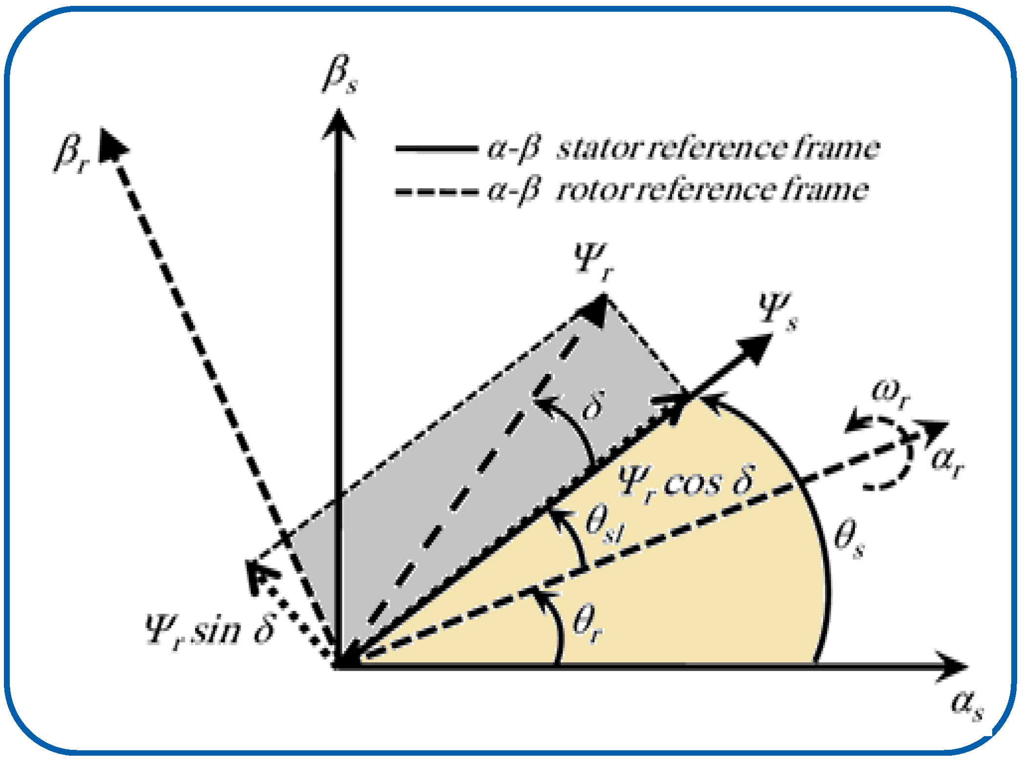
3.1. Stator Flux Estimation

DTC stator flux estimate is among the primary challenges that determine the accuracy and stability of the drive’s operation, since it’s not measured. The simplest solution is the pure integrator-based stator flux estimator voltage model, but it is susceptible to numerous problems [43]: (i) sensitivity in respecting to the dc-drift present in the pure integrator input that causes saturation of the integrator, and (ii) pure integrator initial conditions that cause an unwanted dc deviation in the estimation stator flux signal. We can rewrite AFOO in Equation (15) for IM model assumed in Equations (8)–(11) with the core-loss compensation concept as follows, in order to prevent the dc offset issue:

$$\left\{\begin{array}{c} p {\overrightarrow{\hat{\mathrm{i}}}}_{\mathrm{s}}={\hat{\mathrm{A}}}_{11} {\overrightarrow{\hat{\mathrm{I}}}}_{\mathrm{s}}+({\hat{\mathrm{A}}}_{12}+{\mathrm{D}}_1){\overrightarrow{\hat{\mathrm{\Psi }}}}_{\mathrm{r}}+B {\mathrm{v}}_{\mathrm{s}}+{\mathrm{H}}_{\mathrm{s}} \left({\hat{\mathrm{i}}}_{\mathrm{s}}-{\mathrm{i}}_{\mathrm{s}}\right) \\ p {\overrightarrow{\hat{\mathrm{\Psi }}}}_{\mathrm{r}}={\hat{\mathrm{A}}}_{21} {\overrightarrow{\hat{\mathrm{i}}}}_{\mathrm{s}}+({\hat{\mathrm{A}}}_{22}+{\mathrm{D}}_2){\overrightarrow{\hat{\mathrm{\Psi }}}}_{\mathrm{r}}+B {\mathrm{v}}_{\mathrm{s}}+{\mathrm{H}}_{\mathrm{r}} \left({\hat{\mathrm{A}}}_{\mathrm{s}}-{\mathrm{i}}_{\mathrm{s}}\right)\\ {\overrightarrow{\hat{\mathrm{\Psi }}}}_{\mathrm{s}}={\mathrm{L}}_1{\overrightarrow{\hat{\mathrm{A}}}}_{\mathrm{s}}+{\mathrm{L}}_2 {\overrightarrow{\hat{\mathrm{\Psi }}}}_{\mathrm{r}} \end{array}\right.$$

(17)

where, ${\mathrm{L}}_1=\left[\begin{array}{cc}\frac{{\mathrm{L}}_{\mathrm{s}}{\mathrm{L}}_{\mathrm{r}}-{\mathrm{L}}_{\mathrm{m}}{}^2}{{\mathrm{L}}_{\mathrm{r}}}& 0\\ 0& \frac{{\mathrm{L}}_{\mathrm{s}}{\mathrm{L}}_{\mathrm{r}}-{\mathrm{L}}_{\mathrm{m}}{}^2}{{\mathrm{L}}_{\mathrm{r}}}\end{array}\right]$ and ${\mathrm{L}}_2=\left[\begin{array}{cc}\frac{{\mathrm{L}}_{\mathrm{m}}}{{\mathrm{L}}_{\mathrm{r}}}& 0\\ 0& \frac{{\mathrm{L}}_{\mathrm{m}}}{{\mathrm{L}}_{\mathrm{r}}}\end{array}\right]$.

The first benefit of the estimated stator flux in Equation (17) is that there is no need for motor speed statistics to estimate the flux. This reduces any additional errors, particularly at lower frequencies, associated with calculating or even measuring such signals. Another benefit is that estimated stator flux independent on machine resistances that improve drive reliability. Estimated stator flux ${\overrightarrow{\hat{\mathrm{\Psi }}}}_{\mathrm{s}}$ components in stationary ($\mathsf{\alpha }-\mathsf{\beta }$) reference frame depending on estimated rotor flux ${\overrightarrow{\hat{\mathrm{\Psi }}}}_{\mathrm{r}}$ and stator current${\overrightarrow{\hat{\mathrm{i}}}}_{\mathrm{s}}$ in Equation (17) can be stated as:

$$\left\{\begin{array}{c} {\hat{\mathrm{\Psi }}}_{\mathsf{\alpha }\mathrm{s}}=\frac{{\mathrm{L}}_{\mathrm{m}}}{{\mathrm{L}}_{\mathrm{r}}} {\hat{\mathrm{\Psi }}}_{\mathsf{\alpha }\mathrm{r}}+\frac{{\mathrm{L}}_{\mathrm{s}}{\mathrm{L}}_{\mathrm{r}}-{\mathrm{L}}_{\mathrm{m}}{}^2}{{\mathrm{L}}_{\mathrm{r}}} {\hat{\mathrm{i}}}_{\mathsf{\alpha }\mathrm{s}}\\ {\hat{\mathrm{\Psi }}}_{\mathsf{\beta }\mathrm{s}}=\frac{{\mathrm{L}}_{\mathrm{m}}}{{\mathrm{L}}_{\mathrm{r}}} {\hat{\mathrm{\Psi }}}_{\mathsf{\beta }\mathrm{r}}+\frac{{\mathrm{L}}_{\mathrm{s}}{\mathrm{L}}_{\mathrm{r}}-{\mathrm{L}}_{\mathrm{m}}{}^2}{{\mathrm{L}}_{\mathrm{r}}} {\hat{\mathrm{i}}}_{\mathsf{\beta }\mathrm{s}}\end{array}\right.$$

(18)

3.2. Rotor Speed Estimation

The cost and complexity of the system will be effectively minimized by a sensorless system where the velocity is determined instead of measured. One of the key reasons for the success of inverter fed IM drives is that it is possible to use any standard IM without modifications. It is suggested with current and voltage measuring devices that IM speed can be guessed without the need for speed or flux sensors to be mounted. Through traditional AFOO, rotor speed estimate is obtained via conventional adaptation law as in (15) [5,42]:

$${\hat{\mathrm{\omega }}}_{\mathrm{r}}={\mathrm{K}}_{\mathrm{I}\mathsf{\omega }}\underset{0}{\overset{\mathrm{t}}{{\displaystyle \int }}}\left[{\hat{\mathrm{\Psi }}}_{\mathsf{\beta }\mathrm{r}}\left({\mathrm{i}}_{\mathsf{\alpha }\mathrm{s}}-{\hat{\mathrm{i}}}_{\mathsf{\alpha }\mathrm{s}}\right)-{\overrightarrow{\mathrm{\Psi }}}_{\mathsf{\alpha }\mathrm{r}}\left({\mathrm{i}}_{\mathsf{\beta }\mathrm{s}}-{\hat{\mathrm{i}}}_{\mathsf{\beta }\mathrm{s}}\right)\right]\mathrm{dt}$$

(19)

Like MRAs, the proposed scheme would be separated into two key components, which can be seen in Figure 3; each model is supplied with the same input signal ${\overrightarrow{\mathrm{v}}}_{\mathrm{s}}$. Additionally, the adaptive model is tuned by dual closed loops. The first takes into account the error among measured current ${\overrightarrow{\mathrm{i}}}_{\mathrm{s}}$ and estimated ${\overrightarrow{\hat{\mathrm{i}}}}_{\mathrm{s}}$ from (17), while the other considers the adaptively calculated speed (20). The first closed-loop is being responsible for compensating the offsets that have the major source in current sensors. The controller time constant is calibrated proportionally to a speed value for proper compensation over the entire range of IM rotor velocity. Moreover, for two main reasons, the controllers work slowly: to ensure a lack of effect on transient estimation and because it integrates errors through sinusoidal signals. The second closed-loop provides the rotor velocity ${\hat{\mathrm{\omega }}}_{\mathrm{r}}$, calculated on the basis of difference among estimated and measured currents $\mathrm{\Delta }{\overrightarrow{\mathrm{i}}}_{\mathrm{s}}$ multiplied by estimated stator flux conjugate vector $\overrightarrow{{\hat{\mathrm{\Psi }}}_{\mathrm{s}}{}^{*}}$ as per as (17).

$$\left\{\begin{array}{c}{\mathrm{e}}_{\mathsf{\omega }}=\mathrm{I}\mathrm{m} \left(\overrightarrow{{\hat{\mathrm{\Psi }}}_{\mathrm{s}}^{*}}\mathrm{\Delta }{\overrightarrow{\mathrm{i}}}_{\mathrm{s}}\right)={\hat{\mathrm{\Psi }}}_{\mathsf{\beta }\mathrm{s}}\left({\mathrm{i}}_{\mathsf{\alpha }\mathrm{s}}-{\hat{\mathrm{i}}}_{\mathsf{\alpha }\mathrm{s}}\right) -{\hat{\mathrm{\Psi }}}_{\mathsf{\alpha }\mathrm{s}}\left({\mathrm{i}}_{\mathsf{\beta }\mathrm{s}}-{\hat{\mathrm{i}}}_{\mathsf{\beta }\mathrm{s}}\right)\\ {\hat{\mathsf{\omega }}}_{\mathrm{r}}=\left({\mathrm{K}}_{\mathrm{P}\mathsf{\omega }}+\frac{{\mathrm{K}}_{\mathrm{I}\mathsf{\omega }}}{\mathrm{s}}\right).{\mathrm{e}}_{\mathsf{\omega }}\end{array}\right.$$

(20)

3.3. Other Parameter Estimation

IM stator resistance will vary thanks to temperature change during operation. To provide stator resistance estimation, adaptive control observer could be extended. According to the same Lyapunov’s theory, stator resistance${\mathrm{R}}_{\mathrm{s}}$can also be estimated like rotor speed via a PI controller [39].

$$\left\{\begin{array}{c}{\mathrm{e}}_{{\mathrm{R}}_{\mathrm{s}}}= {\hat{\mathsf{i}}}_{\mathsf{\alpha }\mathrm{s}}\left({\hat{\mathsf{i}}}_{\mathsf{\alpha }\mathrm{s}}-{\mathrm{i}}_{\mathsf{\alpha }\mathrm{s}}\right)+{\hat{\mathsf{i}}}_{\mathsf{\beta }\mathrm{s}}\left({\hat{\mathsf{i}}}_{\mathsf{\beta }\mathrm{s}}-{\mathrm{i}}_{\mathsf{\beta }\mathrm{s}}\right)\\ {\hat{\mathsf{R}}}_{\mathrm{s}}=\left({\mathrm{K}}_{{\mathrm{PR}}_{\mathrm{s}}}+\frac{{\mathrm{K}}_{{\mathrm{IR}}_{\mathrm{s}}}}{\mathrm{s}}\right). {\mathrm{e}}_{{\mathrm{R}}_{\mathrm{s}}}\end{array}\right.$$

(21)

In addition to the temperature variation effect on stator resistance, various parameters in the suggested observer will also adjust during operation. Owing to magnetic saturation, parameters$L_s$;$L_r$ and $L_m$ differ. Although magnetic saturation variance can be compensated for through the nonlinear magnetic model, rotor resistance variation would have a significant effect on the speed-accuracy of our adaptive observer.

It is recognized that the misestimating of ${\mathrm{R}}_{\mathrm{r}}$gives correct estimates of the rotor and stator fluxes during-steady state, but results in a speed misestimating [44]. Rotor resistance estimate can be incorporated into adaptive observer using the approach followed in [42] or IM thermal model. The influence of the core-loss on the estimation of both stator and rotor resistance and its compensation has been well defined in our previous work [45]. Stator current and rotor flux error estimation can give rotor resistance estimate utilizing Lyapunov theory via the suggested AFOO in (17) as:

$$\left\{\begin{array}{c}{\mathrm{e}}_{{\mathrm{R}}_{\mathrm{r}}}= ({\hat{\mathrm{\Psi }}}_{\mathsf{\alpha }\mathrm{r}}-{\mathrm{L}}_{\mathrm{m}}{\hat{\mathrm{i}}}_{\mathsf{\alpha }\mathrm{s}})\left({\mathrm{i}}_{\mathsf{\alpha }\mathrm{s}}-{\hat{\mathrm{i}}}_{\mathsf{\alpha }\mathrm{s}}\right)+({\hat{\mathrm{\Psi }}}_{\mathsf{\beta }\mathrm{r}}-{\mathrm{L}}_{\mathrm{m}}{\hat{\mathrm{i}}}_{\mathsf{\beta }\mathrm{s}})\left({\mathrm{i}}_{\mathsf{\beta }\mathrm{s}}- {\hat{\mathrm{i}}}_{\mathsf{\beta }\mathrm{s}}\right)\\ {\hat{\mathrm{i}}}_{\mathrm{r}}=\left({\mathrm{K}}_{{\mathrm{PR}}_{\mathrm{r}}}+\frac{{\mathrm{K}}_{{\mathrm{IR}}_{\mathrm{r}}}}{\mathrm{s}}\right). {\mathrm{e}}_{{\mathrm{R}}_{\mathrm{r}}}\end{array}\right.$$

(22)

3.4. Torque Estimation

In this analysis, the proposed AFOO can also be used to determine the electromagnetic torque to reduce the error between the reference and desired motor output torque based on estimated stator current and flux. Delay between acquisition time and application time is important to be considered.

$${\hat{\mathrm{T}}}_{\mathrm{e}}=\frac{3}{2}\mathrm{P}\mathrm{Im}\left(\overrightarrow{{\hat{\mathrm{\Psi }}}_{\mathrm{s}}^{*}}{\overrightarrow{\hat{\mathrm{i}}}}_{\mathrm{s},\mathrm{k}-1}\right)$$

(23)

where $\mathrm{k}$ is the sampling time index.

As indicated in Figure 4, our proposed observer can easily estimate stator flux angle as:

$${\hat{\mathsf{\theta }}}_{\mathrm{s}}={\tan }^{-1}\left(\frac{{\hat{\mathrm{\Psi }}}_{\mathsf{\beta }\mathrm{s}}}{{\hat{\mathrm{\Psi }}}_{\mathsf{\alpha }\mathrm{s}}}\right)$$

(24)

The angular speed of stator flux linkage relative to rotor flux linkage may also be computed as:

$$\hat{\mathsf{\delta }}={\tan }^{-1}\left(\frac{{\hat{\mathrm{\Psi }}}_{\mathsf{\beta }\mathrm{r}}}{{\hat{\mathrm{\Psi }}}_{\mathsf{\alpha }\mathrm{r}}}\right)-{\hat{\mathsf{\theta }}}_{\mathrm{s}}$$

(25)

To incorporate the system (17) into the digital processor, it is crucial to acquire a discrete-time state-space representation of proposed system. It should be noted that matrix $\hat{\mathrm{A}}$depending on instantaneous calculated rotor speed value ${\hat{\mathsf{\omega }}}_{\mathrm{r}}$making $\hat{\mathrm{A}}=\hat{\mathrm{A}}\left({\hat{\mathsf{\omega }}}_{\mathrm{r}}\left(\mathrm{t}\right)\right)$ as a linear time-varying system. Time dependence implies that variation of${\mathsf{\omega }}_{\mathrm{r}}$, the offline numerical estimate of discrete-time equivalent system cannot be obtained. The solution would be to achieve a discrete-time varying method that can then be modified with the new estimated value of ${\hat{\mathsf{\omega }}}_{\mathrm{r}}$ at every sampling period. A direct computation or Euler approximation (first-order sequence expansion) [46] are the more popular methods of obtaining the representation of sampled-data for the model. The approximation of Euler is an easy way of obtaining the discrete-time model with a similar response of dynamic behavior. The direct computation of state trajectory in (17) may not be simple as Euler approximation of the first order but gives a more precise representation in the discrete-time (for example, see [47] and references therein).

3.5. Conventional MPTC

For conventional MPTC, just one voltage vector is chosen and not applied till the next control time owing to the updated mechanism for modern microprocessors. The conventional MPTC diagram shown is in Figure 5. Using a PI controller, torque reference would be created via an outer speed control loop and stator flux reference is kept constant at asset value since field weakening and efficiency optimization process are not taken into account in this procedure [29]. In MPTC technique, torque and stator flux are being predicted for all possible voltage vectors supplied by the inverter based on the system model. Then, the best one is decided by minimizing an objective cost function consisting of a torque-flux tracking error.

3.6. Conventional MPFC

Torque and stator flux references are equivalently transformed into single reference for stator flux vector in this process. The MPFC diagram can be seen in Figure 6.

3.7. Proposed MPTFC

MPTC’s cost function is generally defined as a linear combination with torque-flux errors to determining the finest voltage vector, that is defined as:

$${\mathrm{G}}_1=\left|{\mathrm{T}}_{\mathrm{e}}^{\mathrm{ref}}-T_{e,k+1}^p\right|+{\mathsf{\lambda }}_{\mathrm{\Psi }}\left|{\mathrm{\Psi }}_{\mathrm{s}}^{\mathrm{ref}}-{\overrightarrow{\mathrm{\Psi }}}_{s,k+1}^p\right|$$

(26)

where ${\mathsf{\lambda }}_{\mathrm{\Psi }}$is stator flux’s weighting factor in MPTC. Stator flux weighting factor is calibrated in actual time to achieve minimum torque ripple, as suggested in [13]. The weighting factor ${\mathsf{\lambda }}_{\mathrm{\Psi }}$ value has a decisive role in containing the unavoidable ripples if it properly chosen. Therefore, the ${\mathsf{\lambda }}_{\mathrm{\Psi }}$ value must be correctly selected, which requires an online optimization process to choose the optimum value, which results in a further increase in the microcontroller’s computational burden. To avoid the use of weighting factor in MPTC, a new stator flux reference based upon IM model is suggested in [28], which is equivalent to the original reference of torque and stator flux. To pick the finest voltage vector amongst the feasible ones, MPFC’s cost function described in (27) is minimized.

$${\mathrm{G}}_2=\left|{\mathrm{\Psi }}_{\mathrm{s}}^{\mathrm{ref}}-{\overrightarrow{\mathrm{\Psi }}}_{s,k+1}^p\right|$$

(27)

It is clear that the weighting factor will be no longer needed, since only stator flux vector tracking error is involved. The key shortcoming of this technique is that it relies on reference flux angle estimate by using inverse-trigonometric function, which fails to estimate the angle during particular operating conditions [28].

Most often for MPTC and MPFC drives, stator flux reference ${\mathrm{\Psi }}_{\mathrm{s}}^{\mathrm{ref}}$ is usually set constant to its rated value as:

$${\mathrm{\Psi }}_{\mathrm{s}}^{\mathrm{ref}}=\left|{\mathrm{\Psi }}_{\mathrm{s}}^{\mathrm{ref}}\right|$$

(28)

In order to accurately regulate torque and stator flux, we propose the MPTFC design in Figure 7 where the predictive values of stator flux, current and torque are based on suggested AFOO in (17).

MPTFC model predicts electromagnetic torque and stator flux vector’s magnitude at next step in discrete-time $\mathrm{k}+1$as a switch position function to determine ${\mathrm{v}}_{\mathrm{opt}}$ at the present time step$\mathrm{k}$. Prediction accuracy of MPCC and MPTFC, is main issue, as he process of prediction begins with the sampled of measured currents. Unless the measuring and sampling processes were not performed well, noise level will increase, which will then be reflected in the expected values and hence exacerbate voltage selection process, which eventually results in greater ripple content. To avoid that problem, we assume both prediction of torque-flux is dependent on stator currents estimate instead of the measured one.

Integrating estimated stator current in (17) with Euler method from $\mathrm{t}={\mathrm{k}\mathrm{T}}_{\mathrm{s}}$ to $\mathrm{t}=\left(\mathrm{k}+1\right){\mathrm{T}}_{\mathrm{s}}$ and inserting (1) into it relates to the representation of discrete-time:

$${\overrightarrow{\hat{\mathrm{\Psi }}}}_{s,k+1}^p={\overrightarrow{\hat{\mathrm{\Psi }}}}_{\mathrm{s},\mathrm{k}}+{\mathrm{T}}_{\mathrm{s}}{\overrightarrow{\mathrm{v}}}_{\mathrm{s},\mathrm{k}}\left(\mathrm{i}\right)-{\hat{\mathrm{R}}}_{\mathrm{S}} {\mathrm{T}}_{\mathrm{s}} {\overrightarrow{\hat{\mathrm{i}}}}_{\mathrm{s},\mathrm{k}}$$

(29)

Hence, predicted stator flux appears as an estimated function.

$${\overrightarrow{i}}_{s,k+1}^{ p}=\left(1+\frac{{\mathrm{T}}_{\mathrm{s}}}{{\mathsf{\tau }}_{\mathsf{\sigma }}}\right){\overrightarrow{\hat{\mathrm{i}}}}_{\mathrm{s},\mathrm{k}}+\frac{{\mathrm{T}}_{\mathrm{s}}}{{\mathsf{\tau }}_{\mathsf{\sigma }}+{\mathsf{\tau }}_{\mathrm{s}}}\left\{\frac{1}{{\mathrm{R}}_{\mathsf{\sigma }}}\left[\left(\frac{{\mathrm{k}}_{\mathrm{r}}}{{\mathsf{\tau }}_{\mathrm{r}}}-{\mathrm{k}}_{\mathrm{r}}{\mathrm{j}\hat{\mathsf{\omega }}}_{\mathrm{r}}\right){\overrightarrow{\hat{\mathrm{\Psi }}}}_{\mathrm{r},\mathrm{k}}+{\overrightarrow{\mathrm{v}}}_{\mathrm{s},\mathrm{k}}\left(\mathrm{i}\right)\right]\right\}$$

(30)

where${\mathsf{\tau }}_{\mathrm{r}}=\frac{{\mathrm{L}}_{\mathrm{r}}}{{\hat{\mathrm{R}}}_{\mathrm{r}}}$,${\mathrm{k}}_{\mathrm{r}}=\frac{{\mathrm{L}}_{\mathrm{m}}}{{\mathrm{L}}_{\mathrm{r}}}$,${\mathrm{k}}_{\mathrm{s}}=\frac{{\mathrm{L}}_{\mathrm{m}}}{{\mathrm{L}}_{\mathrm{s}}}$,${\mathrm{R}}_{\mathsf{\sigma }}={\hat{\mathrm{R}}}_{\mathrm{S}}+{\hat{\mathrm{R}}}_{\mathrm{r}}+{\mathrm{k}}_{\mathrm{r}}{}^2$,${\mathsf{\tau }}_{\mathsf{\sigma }}=\frac{{\mathsf{\sigma }\mathrm{L}}_{\mathrm{s}}}{{\mathrm{R}}_{\mathsf{\sigma }}}$,${\mathrm{T}}_{\mathrm{s}}$ is sampling-period and ${\overrightarrow{\mathrm{v}}}_{\mathrm{s}}\left(\mathrm{i}\right)$ corresponding to $7$ dissimilar voltage status, $\mathrm{i}$is from $0$ to $6$.

Predicted torque could be obtained after determining the predicted current and flux with:

$${\mathrm{T}}^{\mathrm{p}}{}_{\mathrm{e},\mathrm{k}+1}=\frac{3}{2}\mathrm{P}\left[{\overrightarrow{\hat{\mathrm{\Psi }}}}_{s,k+1}^p\times {\overrightarrow{i}}_{s,k+1}^{ p}\right]$$

(31)

Therefore, a proper cost function would be developed for the proposed MPTF control centered on${\mathrm{G}}_1$and${\mathrm{G}}_2$ as:

$$\mathrm{G}={\mathsf{\lambda }}_{\mathrm{T}}\left|{\mathrm{T}}_{\mathrm{e}}{}^{\mathrm{ref}}-{\mathrm{T}}^{\mathrm{p}}{}_{\mathrm{e},\mathrm{k}+1}\right|+{\mathsf{\lambda }}_{\mathrm{\Psi }}\left|{\mathrm{\Psi }}_{\mathrm{s}}^{\mathrm{ref}}-{\overrightarrow{\hat{\mathrm{\Psi }}}}_{s,k+1}^p\right|$$

(32)

where, torque-flux weighting coefficients are ${\mathsf{\lambda }}_{\mathrm{T}}$and ${\mathsf{\lambda }}_{\mathrm{\Psi }}$ respectively. All feasible inverter topologies for the seven different flux and torque estimates are applied at every sampling stage. Then these samples are being used for determining the cost function. In one sampling period, a switching state that minimizes the $\mathrm{G}$ value is picked to be implemented. To drive $2-$level-inverter, the switching states are then becoming the output. The flow chart of the whole process is seen within Figure 8.

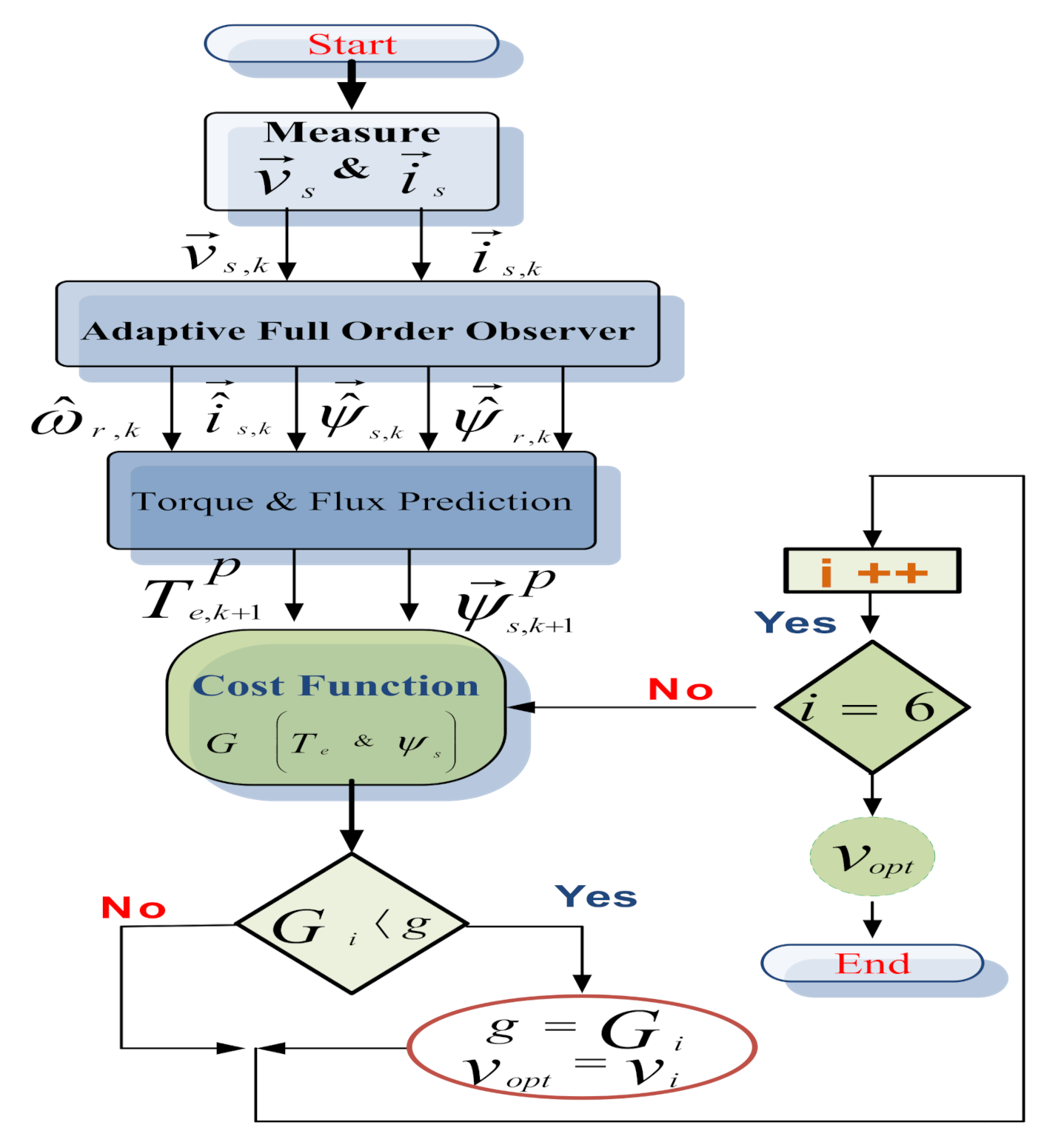
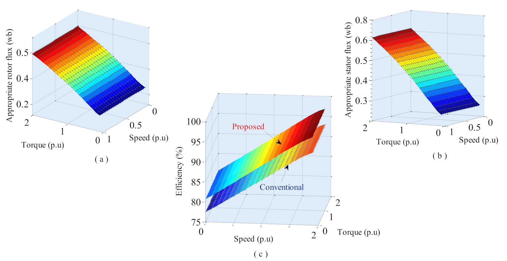
4. Optimal Steady-State Flux for Losses Minimization Criterion

To achieve an optimal stator flux reference for LMC, efficiency optimization is being discussed in this section. IM losses must be precisely defined to obtain a criterion from which whole losses could be minimized. Figure 1 presents the overall IM losses, which consisting of stator copper, rotor copper and core-losses; but not inverter, load, or mechanical losses.

$${\mathrm{P}}_{\mathrm{Loss}}=3\left[{\mathrm{P}}_{\mathrm{cuS}}+{\mathrm{P}}_{\mathrm{cuR}}+{\mathrm{P}}_{\mathrm{fe}}\right]$$

(33)

where ${\mathrm{P}}_{\mathrm{cuS}},{\mathrm{P}}_{\mathrm{cuR}}$are stator and rotor copper losses and ${\mathrm{P}}_{\mathrm{fe}}$ is core-loss.

$${\mathrm{P}}_{\mathrm{cuS}}={\mathrm{R}}_{\mathrm{s}}{\mathrm{I}}_{\mathrm{s}}{}^2={\mathrm{R}}_{\mathrm{s}}\left\{{\mathrm{I}}_{\mathrm{m}}{}^2+{[{\mathrm{I}}_{\mathrm{r}}+\frac{{\mathrm{R}}_{\mathrm{m}}}{{\mathsf{\omega }\mathrm{L}}_{\mathrm{m}}}{\mathrm{I}}_{\mathrm{m}}]}^2\right\}$$

(34)

$${\mathrm{P}}_{\mathrm{cuR}}=\stackrel{‘}{{\mathrm{R}}_{\mathrm{r}}}{\mathrm{I}}_{\mathrm{r}}{}^2={(\frac{{\mathrm{L}}_{\mathrm{m}}}{{\mathrm{L}}_{\mathrm{r}}})}^2{\mathrm{R}}_{\mathrm{r}}{\mathrm{I}}_{\mathrm{r}}{}^2$$

(35)

$${\mathrm{P}}_{\mathrm{fe}}={\mathrm{R}}_{\mathrm{fe}}{\mathrm{I}}_{\mathrm{fe}}{}^2=\frac{{\mathsf{\omega }}^2{\mathrm{L}}_{\mathrm{m}}{}^3}{{\mathrm{L}}_{\mathrm{r}}{\mathrm{R}}_{\mathrm{m}}}{[\frac{{\mathrm{R}}_{\mathrm{m}}}{{\mathsf{\omega }\mathrm{L}}_{\mathrm{m}}}{\mathrm{I}}_{\mathrm{m}}]}^2$$

(36)

Whereas ${\mathrm{R}}_{\mathrm{m}}{}^2\ll {({\mathsf{\omega }\mathrm{L}}_{\mathrm{m}})}^2$, substituting (34) and (36) into (33) yields the total loss expression as:

$$P_{Loss}=3\left\{\left[R_s+\frac{R_m{L}_m}{L_r}\right]I_m{}^2+\left[R_s+{(\frac{L_m}{L_r})}^2{R}_r\right]I_r{}^2+\frac{2R_m{R}_s}{\omega L_m}{I}_m{I}_r\right\}$$

(37)

where $\mathrm{a}={\mathrm{L}}_{\mathrm{m}}/{\mathrm{L}}_{\mathrm{r}}$, ${\mathrm{L}}_{\mathrm{m}}^{\text{′}}={\mathrm{a}\mathrm{L}}_{\mathrm{m}}$, ${\mathrm{R}}_{\mathrm{r}}^{\text{′}}={\mathrm{a}}^2{\mathrm{R}}_{\mathrm{r}}$, ${\mathrm{R}}_{\mathrm{fe}}=\mathrm{a}\frac{{({\mathsf{\omega }\mathrm{L}}_{\mathrm{m}})}^2}{{\mathrm{R}}_{\mathrm{m}}}=\frac{{\mathsf{\omega }}^2{\mathrm{L}}_{\mathrm{m}}{}^3}{{\mathrm{L}}_{\mathrm{r}}{\mathrm{R}}_{\mathrm{m}}}$, ${\mathrm{I}}_{\mathrm{fe}}=\frac{{\mathrm{R}}_{\mathrm{m}}}{{\mathsf{\omega }\mathrm{L}}_{\mathrm{m}}}{\mathrm{I}}_{\mathrm{m}}$and ${\mathrm{I}}_{\mathrm{s}}=\sqrt{{\mathrm{I}}_{\mathrm{m}}{}^2+{({\mathrm{I}}_{\mathrm{r}}+{\mathrm{I}}_{\mathrm{fe}})}^2}$. Direct FOC equations of IM that take core loss into accounts are:

$$\begin{array}{cc}\mathrm{Rotor}\mathrm{flux}:\hfill & {\mathrm{\Psi }}_{\mathrm{r}}^{\text{′}}={\mathrm{L}}_{\mathrm{m}}^{\text{′}}{\mathrm{I}}_{\mathrm{m}}\end{array}$$

(38)

$$\begin{array}{cc}\mathrm{Electromagnetic}\mathrm{torque}:\hfill & {\mathrm{T}}_{\mathrm{e}}=3{\mathrm{P}\mathrm{\Psi }}_{\mathrm{r}}^{\text{′}}{\mathrm{I}}_{\mathrm{r}}\end{array}$$

(39)

$$\begin{array}{cc}\mathrm{Slip}\mathrm{frequency}:\hfill & {\mathsf{\omega }}_{\mathrm{sl}}=R_r \frac{{\mathrm{\Psi }}_{\mathrm{r}}^{\text{′}}}{L_r}\end{array}$$

(40)

The substitution of (38) and (39) into (37) helps us to rewrite the complete loss as:

$${\mathrm{P}}_{\mathrm{Loss}}=3\left\{\left[{\mathrm{R}}_{\mathrm{s}}+\frac{{\mathrm{R}}_{\mathrm{m}}{\mathrm{L}}_{\mathrm{m}}}{{\mathrm{L}}_{\mathrm{r}}}\right]\frac{{\mathrm{L}}_{\mathrm{r}}{}^2}{{\mathrm{L}}_{\mathrm{m}}{}^4}{\left|{\mathrm{\Psi }}_{\mathrm{r}}^{\text{′}}\right|}^2+\left[{\mathrm{R}}_{\mathrm{s}}+{(\frac{{\mathrm{L}}_{\mathrm{m}}}{{\mathrm{L}}_{\mathrm{r}}})}^2{\mathrm{R}}_{\mathrm{r}}\right]\frac{{\mathrm{T}}_{\mathrm{e}}{}^2}{9{\mathrm{P}}^2}{\left|\stackrel{‘}{{\mathrm{\Psi }}_{\mathrm{r}}^{\text{′}}}\right|}^{-2}+\left[\frac{2{\mathrm{R}}_{\mathrm{m}}{\mathrm{R}}_{\mathrm{s}}}{{\mathsf{\omega }\mathrm{L}}_{\mathrm{m}}}\right]\frac{{\mathrm{L}}_{\mathrm{r}}{\mathrm{T}}_{\mathrm{e}}}{3{\mathrm{P}\mathrm{L}}_{\mathrm{m}}{}^2}\right\}$$

(41)

This implies that ${\mathrm{P}}_{\mathrm{Loss}}$ is a variable dependent on rotor flux${\mathrm{\Psi }}_{\mathrm{r}}^{\text{′}}$. Assuming that under constant load torque, none of machine parameters have any dependency upon rotor flux${\mathrm{\Psi }}_{\mathrm{r}}^{\text{′}}$. By setting a derivative of Equation (41) with respect to ${\mathrm{\Psi }}_{\mathrm{r}}^{\text{′}}$ to zero, we could obtain a rotor flux that provides the minimum losses.

$$\frac{\partial {\mathrm{P}}_{\mathrm{Loss}}}{\partial \stackrel{‘}{{\mathrm{\Psi }}_{\mathrm{r}}}}=0$$

(42)

$$\frac{\partial {\mathrm{P}}_{\mathrm{Loss}}}{\partial \left|{\mathrm{\Psi }}_{\mathrm{r}}^{\text{′}}\right|}=3\left\{\begin{array}{c}2 \left[{\mathrm{R}}_{\mathrm{s}}+\frac{{\mathrm{R}}_{\mathrm{m}}{\mathrm{L}}_{\mathrm{m}}}{{\mathrm{L}}_{\mathrm{r}}}\right] \frac{{\mathrm{L}}_{\mathrm{r}}{}^2}{{\mathrm{L}}_{\mathrm{m}}{}^4}\left|{\mathrm{\Psi }}_{\mathrm{r}}^{\text{′}}\right|-\\ 2\left[{\mathrm{R}}_{\mathrm{s}}+{(\frac{{\mathrm{L}}_{\mathrm{m}}}{{\mathrm{L}}_{\mathrm{r}}})}^2{\mathrm{R}}_{\mathrm{r}}\right] \frac{{\mathrm{T}}_{\mathrm{e}}{}^2}{9{\mathrm{P}}^2} {\left|{\mathrm{\Psi }}_{\mathrm{r}}^{\text{′}}\right|}^{-3}\end{array}\right\}$$

(43)

Solving Equation (43) gives us an appropriate rotor flux ${\mathrm{\Psi }}_{\mathrm{r}}^{\text{′} A}$corresponding to the maximum efficiency point, where. $K=\left[{\left(\frac{{\hat{\mathrm{R}}}_{\mathrm{s}}{\mathrm{L}}_{\mathrm{r}}{}^2+{\hat{\mathrm{R}}}_{\mathrm{r}}{\mathrm{L}}_{\mathrm{m}}{}^2}{{\hat{\mathrm{R}}}_{\mathrm{s}}{\mathrm{L}}_{\mathrm{r}}{}^4+{\mathrm{L}}_{\mathrm{m}}{\mathrm{L}}_{\mathrm{r}}{}^3{\mathrm{R}}_{\mathrm{m}}}\right)}^{\frac{1}{4}}\frac{2R_m{R}_s}{\omega L_m}\right].\frac{{\mathrm{L}}_{\mathrm{m}}}{\sqrt{3\mathrm{P}}}$.

$${\mathrm{\Psi }}_{\mathrm{r}}^{\text{′} A}=\mathrm{K}\sqrt{{\mathrm{T}}_{\mathrm{e}}}$$

(44)

Before applying ${\mathrm{\Psi }}_{\mathrm{r}}^{\text{′} A}$ to the direct FOC of IM, the coefficient with estimated parameters must be multiplied as follows:

$${\overrightarrow{\mathrm{\Psi }}}_{r,k}^A=\frac{{\mathrm{L}}_{\mathrm{r}}}{{\mathrm{L}}_{\mathrm{m}}}{\mathrm{\Psi }}_{\mathrm{r}}^{\text{′} A}=\frac{{\mathrm{L}}_{\mathrm{r}}}{{\mathrm{L}}_{\mathrm{m}}}\hat{\mathrm{K}}\sqrt{{\mathrm{T}}_{\mathrm{e}}}$$

(45)

Corresponding suitable stator flux can also be determined based on the steady-state relationship among stator-rotor fluxes as [33]:

$${\overrightarrow{\mathrm{\Psi }}}_{s,k}^A=\sqrt{{\left(\frac{{\mathrm{L}}_{\mathrm{s}}}{{\mathrm{L}}_{\mathrm{m}}}\right)}^2{\overrightarrow{\mathrm{\Psi }}}_{r,k}^A+{\left(\frac{4{\mathsf{\sigma }\mathrm{L}}_{\mathrm{s}}{\mathrm{L}}_{\mathrm{r}}}{3{\mathrm{P}\mathrm{L}}_{\mathrm{m}}}\right)}^2\frac{{\mathrm{T}}_{\mathrm{e}}{}^2}{{\left({\overrightarrow{\mathrm{\Psi }}}_{r,k}^A\right)}^2}}$$

(46)

The optimum stator flux’s reference amplitude required by suggested MPTFC in LMC is provided by Equation (46). Expression of (46) updates (28) as:

$${\mathrm{\Psi }}_{\mathrm{s}}^{\mathrm{ref}}=\left|{\overrightarrow{\mathrm{\Psi }}}_{s,k}^A\right|$$

(47)

It thus completes the data necessary to apply (29) and so the cost function (32).

In order to calculate the efficiency of IM based on the total losses calculated in Equation (41), as in [47]:

$$\mathsf{\eta }=\frac{{\mathrm{P}}_{\mathrm{Out}}}{{\mathrm{P}}_{\mathrm{Out}}+{\mathrm{P}}_{\mathrm{Loss}}}$$

(48)

where $\mathsf{\eta }$ is the efficiency and the output power is ${\mathrm{P}}_{\mathrm{Out}}={\mathsf{\omega }}_{\mathrm{r}} {\mathrm{T}}_{\mathrm{e}}$.

5. System Layout

Complete approach layout is shown in Figure 9. Stator voltages and currents are the measured quantities, that used by suggested AFOO to obtain the estimated values of; rotor velocity${\hat{\mathsf{\omega }}}_{\mathrm{r},\mathrm{k}},$ rotor flux${\overrightarrow{\hat{\mathrm{\Psi }}}}_{\mathrm{r},\mathrm{k}},$ stator current${\overrightarrow{\hat{\mathrm{i}}}}_{\mathrm{s},\mathrm{k}}$, stator flux ${\overrightarrow{\hat{\mathrm{\Psi }}}}_{\mathrm{s},\mathrm{k}}$ and torque ${\hat{\mathrm{T}}}_{\mathrm{e},\mathrm{k}}$ to predict stator flux${\overrightarrow{\hat{\mathrm{\Psi }}}}_{s,k+1}^p$and corresponding predicted torque${\mathrm{T}}_{\mathrm{e},\mathrm{k}+1}^{\mathrm{P}}$. Estimated states are fed back toward the stator flux outer loop and inner loop of the torque to produce stator flux and torque references for cost function in Equation (32). The LMC algorithm provides optimum stator flux’s amplitude; alternatively, stator flux reference could be followed through fed back flux loop. Optimum voltage vector is selected through applying cost function $\mathrm{G}$ on the base of the references and predicted values of both torque and stator flux to complete the suggested MPTFC of IM drive.

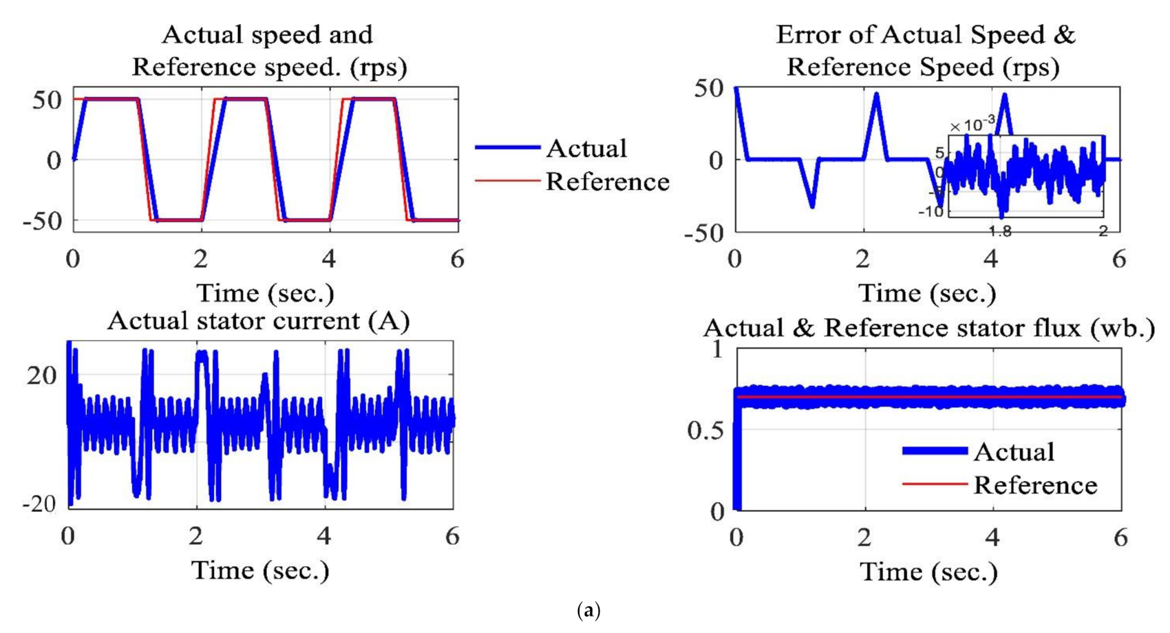
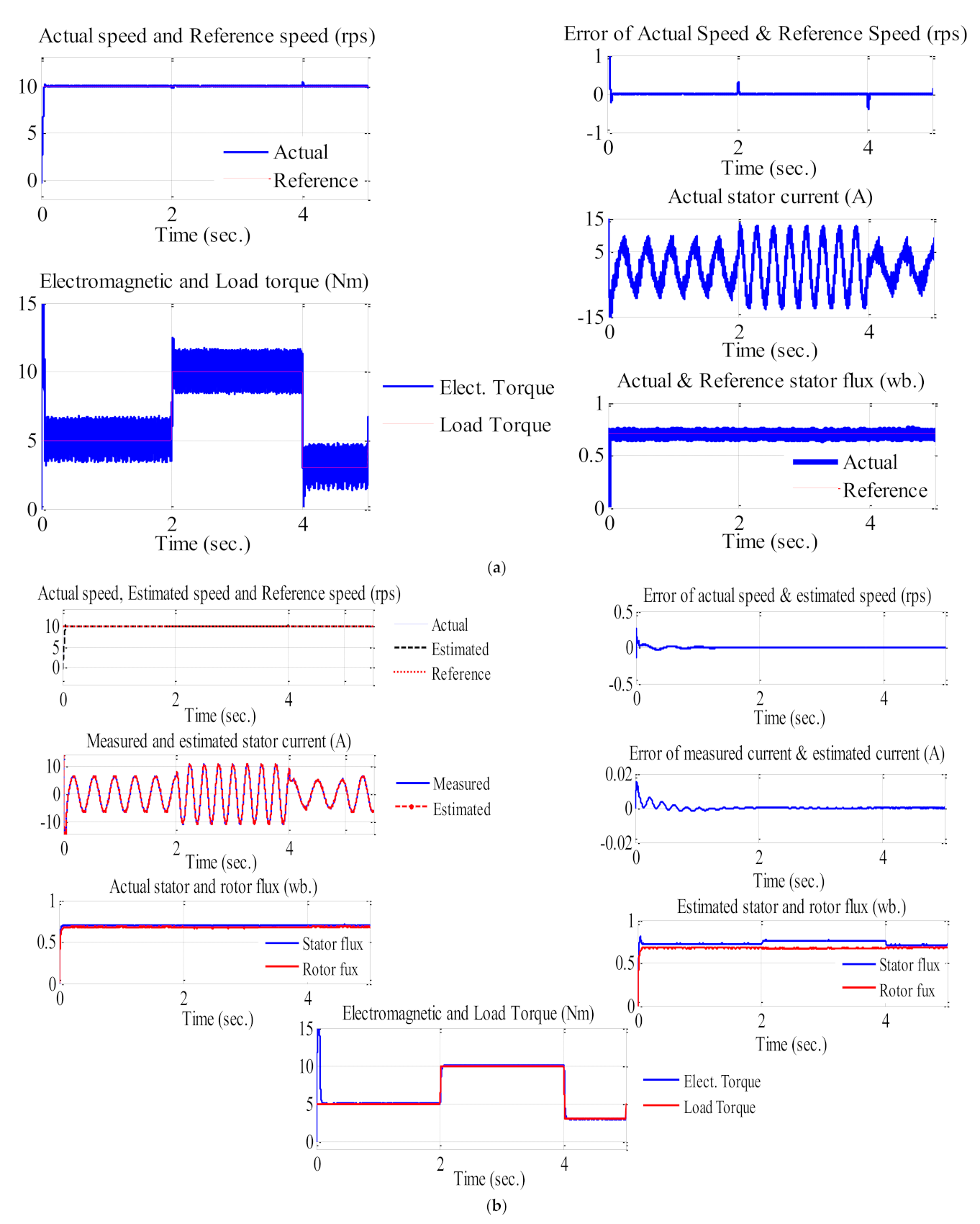
6. Results and Discussion

The suggested MPTFC approach is simulated in MATLAB/Simulink environment to verify its effectiveness. For simplicity, the proposed MPTFC performance is compared to conventional MPTC that utilize cost function $\mathrm{G}1$ in Equation (26) and constant stator flux reference$\left|{\mathrm{\Psi }}_{\mathrm{s}}^{\mathrm{ref}}\right|=0.71\mathrm{wb}$. MPTC technique is referred to as method $\mathrm{I},$ and the proposed one of MPTFC with the modified AFOO is referred to as method $\mathrm{II}$ in the following phrases, respectively. Motor parameters are mentioned in

Table 1. IM Parameters.

Symbol	Parameters	Values
$v_s$	Rated voltage	$380\mathrm{V}$
$n_p$	No. pole pairs	$1$
$f$	Rated frequency	$50\mathrm{Hz}$
$R_s$	Stator resistance	$1.2\mathsf{\Omega }$
$R_r$	Rotor resistance	$1\mathsf{\Omega }$
$L_s$	Stator self-inductance	$175\times {10}^{-3}\mathrm{H}$
$L_r$	Rotor self-inductance	$175\times {10}^{-3}\mathrm{H}$
$L_m$	Magnetizing inductance	$170\times {10}^{-3}\mathrm{H}$
$J$	Moment of inertia	$0.062{\mathrm{Kgm}}^2$
${\Psi }_{sn}$	Nominal stator flux	$0.71\mathrm{wb}$
$T_n$	Nominal torque	$20\mathrm{Nm}$
${\mathrm{R}}_{\mathrm{m}}$	Core-resistance	$2.186\mathrm{K}\mathsf{\Omega }$
${\mathrm{T}}_{\mathrm{s}}$	Sampling-time	$4\times {10}^{-5}\mathrm{s}$

.

The following hints about the simulating system should be noted; the IM has been considered nonlinear and takes the core-loss influence into account. Moreover, the proposed observer-based on the mentioned equations in the paper has been implemented using MATLAB^® and Simulink^® environment. Furthermore, the inverter has been built from the Simulink libraries of Simscape Electrical Specialized Power Systems library. However, no extra band-limited white noise was introduced into the signals.

Figure 10 shows starting response from standstill to $\left(100\mathrm{rps}\right)$for the both methods. Stator flux is first developed using preexcitation, and torque is restricted to $100$ percent rated value ($20\mathrm{Nm}$) during the accelerating stage. An external load with $50\%$ of the nominal value ($10\mathrm{Nm}$) is suddenly applied at ($\mathrm{t}=0.7\mathrm{s})$ to the tested IM. In MPTC, actual speed is compared with speed reference unlike in the proposed system which utizes estimate speed.

Curves shown in Figure 10, through top to bottom are velocity, torque, stator flux and stator current, respectively. It is obviously seen that in low-speed operation, proposed MPTFC works well and exhibits high robustness regarding load disturbance. It can also be observed that method $\mathrm{I}$ has similar dynamic performance, but it produces much higher flux, current and torque ripples.

A more extensive steady-state torque, current and stator flux waveforms with $\left(50\%\right)$ of rated torque ($10\mathrm{Nm}$) is shown in Figure 11. The ripples of torque, current and stator flux in method $\mathrm{II}$ are shown to be much smaller than in method$\mathrm{I}$, demonstrating the efficiency of suggested approach of MPTFC.

Conventional and suggested drive responses are shown in Figure 12a,b throughout speed reversals. It could be said that the motor accelerates rapidly from ($50\mathrm{rps}$) to ($-50\mathrm{rps}$) for three full cycles of forward and reverse speed to test the drive performance in low and reverse speed operation. The load torque is held constant at ($5\mathrm{Nm}$) during the whole test period. The conventional MPTC works at reverse speed operation while it suffers from unwanted ripples in the flux, torque and the stator currents when compared to the proposed method, as shown in Figure 12a. Moreover, an acceptable error between actual, estimated velocity and measured one is shown in Figure 12b. Furthermore, the error between the estimated stator current and actual ones through our proposed drive is shown in Figure 12b, which validates the proposed observer’s operation. The actual and estimate values of stator and rotor fluxes throughout the reverse speed operation are also shown in Figure 12b. Figure 12c shows the comparison of the response of the stator currents and stator flux with the operation of speed reversal at ($50\mathrm{rps}$) between the conventional MPTC and the proposed MPTFC. The figure proves that the response of the flux and stator currents with the proposed MPTFC is better than those of the conventional MPTC.

Furthermore, the drive responses of the conventional and proposed method under step change of the load disturbance are shown in Figure 13a,b at a very low speed operating range of ($10\mathrm{rps}$). A load torque of ($5\mathrm{Nm}$) is applied at starting, then load torque is increased to ($10\mathrm{Nm}$) at ($\mathrm{t}=2\mathrm{s}$) then decreased to ($3\mathrm{Nm}$) at ($\mathrm{t}=4\mathrm{s}$) and finally back to ($5\mathrm{Nm}$). Figure 13a shows a similar dynamic performance of MPTC at load disturbance; nevertheless, it produces greatly higher flux, current, and torque ripples when comparing it to the proposed MPTFC. Actual values of stator and rotor fluxes are very robust in the suggested drive, as they were compensated by the estimated value of the stator flux, as shown in Figure 13b. Moreover, both speed and current error can be seen as a rather pleasant feature, demonstrating high robustness against external load disturbance of the proposed MPTFC. It is also obvious that the both conventional and proposed method currents in Figure 13a,b seem to be quite sinusoidal in shape. Moreover, Figure 13c displays the comparison of the response of the stator currents, stator flux, and torque with the operation of load disturbance at ($10\mathrm{rps}$) between the conventional MPTC and the proposed MPTFC. The figure verifies that the response of the flux, stator currents and torque with the proposed MPTFC is better than those of the conventional MPTC.

In the second case, the IM being controlled under the suggested MPTFC with applying of LMC, where stator flux’s reference is adjusted to optimal or appropriate flux ${\overrightarrow{\mathrm{\Psi }}}_{s,k}^A$ which is determined in (46) to obtain the highest efficiency or lowest losses. Figure 14a indicates total steady-state losses of IM; the conventional method is represented by dashed lines, while the proposed method is represented by solid lines at various values of speed. Overall loss operated throughout suggested method is certainly smaller than that of the conventional method with constant flux at each motor speed. It is obvious that, as can be seen in Figure 14b, the rotor flux where the losses are minimal depends upon load torque. In most other words, rotor flux that provides maximum IM efficiency stands as a function of load torque.

Optimal rotor flux for maximum operating efficiency that calculated in (45), is drawn in Figure 15 for various driving conditions. It is influenced by motor speed since the core-loss is taken into account. This implies that rotor flux drops to decrease the core-loss, which raises through the excitation frequency further than the other loses at high speeds. Corresponding optimal stator flux for minimum losses that calculated in (46), is drawn in Figure 15b.

IM steady-state efficiency with constant rotor flux is plotted with dash lines and also solid lines represents optimal suggested method, that shown in Figure 15c. It clearly shows that suggested method here achieves higher efficiency over large range of load torques owing to adjusting rotor flux rendering to torque. Thus, it can be said that the proposed system efficiency with LMC has improved significantly in excess of the classical one.

To investigate dynamic performance, load torque will varied as in case of load disturbance in Figure 13 and IM speed is kept constant with very low amount ($10\mathrm{rps}$). Stator flux’s reference is held at its rated value ($0.71\mathrm{wb}$) for MPTC and suggested estimated value for MPTFC without the LMC. For the suggested MPTFC with LMC, stator flux’s reference is adjusted on line through optimal value, which is also presented in Figure 16.

The steady-state optimal flux, which achieves minimum steady-state losses, varies with the operating conditions. To achieve balance among copper and iron losses, it rises with torque and decreases as rotor speed increases.

In the proposed MPTFC with LMC, the optimal stator flux, that calculated in Equation (46), achieves minimum losses, and varies with the operating conditions. To achieve balance among copper and iron losses, it rises with the torque and decreases as rotor speed increases. It can also be seen from Figure 16, in which a comparison of the three control procedures is demonstrated, that proposed MPTFC (without and with LMC) exhibits better dynamic behavior compared to MPTC technique.

In addition, it should be noted that losses are effectively minimized during light loading when following the LMC approach and consequently, IM drive efficiency is improved, as clearly seen in Figure 16.

To clarify the speed response throughout low-speed region, that considered among the most major aspects of this study, actual speeds is compared for MPTC and suggested MPTFC (without and with LMC) approaches in Figure 17. Step change to reference speed at ($\mathrm{t}=0.05\mathrm{s})$ from $\left(0\mathrm{rps}\right)$ to $\left(10\mathrm{rps}\right)$is applied with constant load torque$(5\mathrm{Nm}$). Figure 17 shows a step response of the conventional MPTC and the proposed one of MPTFC with and without considering LMC. To clarify these values more precisely, the over shot, rise time, and settling time were calculated in

Table 2. Values of the over shot, rise time, and settling time for MPTC and suggested MPTFC (without and with LMC) approaches.

Method	Over Shot (%)	Rise Time	Settling Time
MPTC	$2.8$	$0.0399$	$0.0952$
MPTFC	$1.1$	$0.0394$	$0.0541$
MPTFC + LMC	$1.5$	$0.0639$	$0.1183$

. The results show that the overshot of proposed one of MPTFC with LMC is better than those of the conventional one and the proposed MPTFC without LMC. Moreover, the figure shows an increasing in the rise time and settling time of the MPTFC with LMC. Moreover, in general, the speed response of the three schemes is stable as shown in time domine analysis of Figure 17.

7. Conclusions

Paper proposed a new MPTFC solution for $2-$level inverter-fed IM drives to address the torque-ripple-phenomenon issue in MPTC. A novel design for sensorless observer centered on AFOO has been proposed. Stator flux estimation in the robust suggested observer provides a strong torque response during very low-speed operations. By introducing the recommended approach, much better steady-state stability in terms of flux/torque ripples is being observed without disturbing the dynamic response. In our proposed MPTFC, a closed feedback-loop is added to the suggested drive; consequently, uncertainties (error of estimated speed, unbalance current measurement and variance of parameters) are being compensated. Therefore, the proposed prediction approach was conducted more accurately. Moreover, the loss-minimization-criterion (LMC) is imposed that minimizes IM losses, particularly at low-speed and light loading, thus improving drive efficiency. In addition to minimizing the losses during steady-state operations, the comparative results affirm the proposed MPTFC effectiveness in achieving fewer oscillations. The proposed MPTFC approach improves IM drive robustness significantly. Finally, it should be noted that the experimental validations of the proposed control system should be considered in future work, which is not considered because of the lack of laboratory equipment and apparatus and the conditions of COVID-19.

References

1. Schauder, C. Adaptive speed identification for vector control of induction motors without rotational transducers. In Conference Record of the IEEE Industry Applications Society Annual Meeting; IEEE: Piscataway, NJ, USA; pp. 493–499.
2. Diab, A.A.Z. Novel robust simultaneous estimation of stator and rotor resistances and rotor speed to improve induction motor efficiency. Int. J. Power Electron. 2017, 8, 267–287. [Google Scholar] [CrossRef]
3. Kumar, R.; Das, S.; Chattopadhyay, A.K. Comparative assessment of two different model reference adaptive system schemes for speed-sensorless control of induction motor drives. IET Electr. Power Appl. 2016, 10, 141–154. [Google Scholar] [CrossRef]
4. Blasco-Gimenez, R.; Asher, G.; Sumner, M.; Bradley, K. Dynamic performance limitations for MRAS based sensorless induction motor drives. Part 1: Stability analysis for the closed loop drive. IEE Proc. Electr. Power Appl. 1996, 143, 113–122. [Google Scholar] [CrossRef]
5. Kubota, H.; Matsuse, K.; Nakano, T. DSP-based speed adaptive flux observer of induction motor. IEEE Trans. Ind. Appl. 1993, 29, 344–348. [Google Scholar] [CrossRef]
6. Verghese, G.C.; Sanders, S.R. Observers for flux estimation in induction machines. IEEE Trans. Ind. Electron. 1988, 35, 85–94. [Google Scholar] [CrossRef]
7. Harnefors, L. Design and analysis of general rotor-flux-oriented vector control systems. IEEE Trans. Ind. Electron. 2001, 48, 383–390. [Google Scholar] [CrossRef]
8. Casadei, D.; Profumo, F.; Serra, G.; Tani, A. FOC and DTC: Two viable schemes for induction motors torque control. IEEE Trans. Power Electron. 2002, 17, 779–787. [Google Scholar] [CrossRef] [Green Version]
9. Diab, A.A.Z.; Selim, S.; Elnaghi, B.E. Particle swarm optimization based vector control of permanent magnet synchronous motor drive. In IEEE NW Russia Young Researchers in Electrical and Electronic Engineering Conference (EIConRusNW); IEEE: Piscataway, NJ, USA, 2016; pp. 740–746. [Google Scholar]
10. Alsofyani, I.M.; Idris, N.R.N. Simple flux regulation for improving state estimation at very low and zero speed of a speed sensorless direct torque control of an induction motor. IEEE Trans. Power Electron. 2015, 31, 3027–3035. [Google Scholar] [CrossRef]
11. Geyer, T.; Papafotiou, G.; Morari, M. Model predictive direct torque control—Part I: Concept, algorithm, and analysis. IEEE Trans. Ind. Electron. 2008, 56, 1894–1905. [Google Scholar] [CrossRef]
12. Rodríguez, J.; Kennel, R.M.; Espinoza, J.R.; Trincado, M.; Silva, C.A.; Rojas, C.A. High-performance control strategies for electrical drives: An experimental assessment. IEEE Trans. Ind. Electron. 2011, 59, 812–820. [Google Scholar] [CrossRef]
13. Rojas, C.A.; Rodriguez, J.; Villarroel, F.; Espinoza, J.R.; Silva, C.A.; Trincado, M. Predictive torque and flux control without weighting factors. IEEE Trans. Ind. Electron. 2012, 60, 681–690. [Google Scholar] [CrossRef]
14. Diab, A.A.Z.; Kotin, D.A.; Pankratov, V.V. Speed control of sensorless induction motor drive based on model predictive control. In 14th International Conference of Young Specialists on Micro/Nanotechnologies and Electron Devices; IEEE: Piscataway, NJ, USA, 2013; pp. 269–274. [Google Scholar]
15. Nacusse, M.A.; Romero, M.; Haimovich, H.; Seron, M.M. DTFC versus MPC for induction motor control reconfiguration after inverter faults. In Conference on Control and Fault-Tolerant Systems (SysTol); IEEE, Piscataway, NJ, USA, 2010; pp. 759–764. [Google Scholar]
16. Wang, T.; Zhu, J. Finite-control-set model predictive direct torque control with extended set of voltage space vectors. In 2017. In 20th International Conference on Electrical Machines and Systems (ICEMS); IEEE: Piscataway, NJ, USA, 2017; pp. 1–6. [Google Scholar]
17. Zhang, Y.; Wang, Q.; Liu, W. Direct torque control strategy of induction motors based on predictive control and synthetic vector duty ratio control. In International Conference on Artificial Intelligence and Computational Intelligence; IEEE: Piscataway, NJ, USA, 2010; Volume 2, pp. 96–101. [Google Scholar]
18. Lunardi, A.; Sguarezi, A. Experimental results for predictive direct torque control for a squirrel cage induction motor. In Brazilian Power Electronics Conference (COBEP); IEEE: Piscataway, NJ, USA, 2017; pp. 1–5. [Google Scholar]
19. Kumar, P.; Rathore, V.; Yadav, K. Calculation of Torque Ripple and Derating Factor of a Symmetrical Six-Phase Induction Motor (SSPIM) Under the Loss of Phase Conditions. In Nanoelectronics. In Circuits and Communication Systems; Springer: Berlin/Heidelberg, Germany, 2021; pp. 441–453. [Google Scholar]
20. ML, P.; Eshwar, K.; Thippiripati, V.K. A modified duty-modulated predictive current control for permanent magnet synchronous motor drive. IET Electr. Power Appl. 2021, 15, 25–38. [Google Scholar]
21. Jing, K.; Liu, C.; Lin, X. Discrete Dynamical Predictive Control on Current Vector for Three-Phase PWM Rectifier. J. Electr. Eng. Technol. 2021, 16, 267–276. [Google Scholar] [CrossRef]
22. Lakhimsetty, S.; Somasekhar, V.T. An Efficient Predictive Current Control Strategy for a Four-Level Open-End Winding Induction Motor Drive. IEEE Trans. Power Electron. 2019, 35, 6198–6207. [Google Scholar] [CrossRef]
23. Xue, Y.; Meng, D.; Yin, S.; Han, W.; Yan, X.; Shu, Z.; Diao, L. Vector-based model predictive hysteresis current control for asynchronous motor. IEEE Trans. Ind. Electron. 2019, 66, 8703–8712. [Google Scholar] [CrossRef]
24. Miranda, H.; Cortés, P.; Yuz, J.I.; Rodríguez, J. Predictive torque control of induction machines based on state-space models. IEEE Trans. Ind. Electron. 2009, 56, 1916–1924. [Google Scholar] [CrossRef]
25. Diab, A.Z.; Kotin, D.; Anosov, V.; Pankratov, V. A comparative study of speed control based on MPC and PI-controller for Indirect Field oriented control of induction motor drive. In 12th International Conference on Actual Problems of Electronics Instrument Engineering (APEIE); IEEE: Piscataway, NJ, USA, 2014; pp. 728–732. [Google Scholar]
26. Rodriguez, J.; Cortes, P. Predictive Control of Power Converters and Electrical Drives; John Wiley & Sons: Hoboken, NJ, USA, 2012; Volume 40. [Google Scholar]
27. Davari, S.A.; Khaburi, D.A.; Kennel, R. An improved FCS–MPC algorithm for an induction motor with an imposed optimized weighting factor. IEEE Trans. Power Electron. 2011, 27, 1540–1551. [Google Scholar] [CrossRef]
28. Zhang, Y.; Yang, H. Model-predictive flux control of induction motor drives with switching instant optimization. J. IEEE Trans. Energy Convers. 2015, 30, 1113–1122. [Google Scholar] [CrossRef]
29. Zhang, Y.; Yang, H.; Xia, B. Model-predictive control of induction motor drives: Torque control versus flux control. IEEE Trans. Ind. Appl. 2016, 52, 4050–4060. [Google Scholar] [CrossRef]
30. Karamanakos, P.; Geyer, T. Model predictive torque and flux control minimizing current distortions. IEEE Trans. Power Electron. 2018, 34, 2007–2012. [Google Scholar] [CrossRef]
31. Geyer, T. Algebraic tuning guidelines for model predictive torque and flux control. IEEE Trans. Ind. Appl. 2018, 54, 4464–4475. [Google Scholar] [CrossRef]
32. Geyer, T. Model Predictive Control of High Power Converters and Industrial Drives; John Wiley & Sons: Hoboken, NJ, USA, 2016. [Google Scholar]
33. El Fadili, A.; Giri, F.; El Magri, A.; Lajouad, R.; Chaoui, F.Z. Towards a global control strategy for induction motor: Speed regulation, flux optimization and power factor correction. Int. J. Electr. Power Energy Syst. 2012, 43, 230–244. [Google Scholar] [CrossRef] [Green Version]
34. Diab, A.Z.; Vdovin, V.; Kotin, D.; Anosov, V.; Pankratov, V. Cascade model predictive vector control of induction motor drive. In 12th International Conference on Actual Problems of Electronics Instrument Engineering (APEIE); IEEE: Piscataway, NJ, USA, 2014; pp. 669–674. [Google Scholar]
35. Borisevich, A.; Schullerus, G. Energy efficient control of an induction machine under torque step changes. IEEE Transactions Energy Convers. 2016, 31, 1295–1303. [Google Scholar] [CrossRef]
36. Ta, C.-M.; Hori, Y. Convergence improvement of efficiency-optimization control of induction motor drives. IEEE Trans. Ind. Appl. 2001, 37, 1746–1753. [Google Scholar]
37. Tang, Y. Flux Controlled Motor Management. U.S. Patent 20100090629A1, 14 June 2011. [Google Scholar]
38. Diab, A.A.Z. Robust simultaneous estimation of stator and rotor resistances and rotor speed for predictive maintenance of sensorless induction motor drives. Int. J. Power Energy Convers. 2017, 8, 411–434. [Google Scholar] [CrossRef]
39. Diab, A.A.Z. Implementation of a novel full-order observer for speed sensorless vector control of induction motor drives. Electr. Eng. 2017, 99, 907–921. [Google Scholar] [CrossRef]
40. Matsuse, K.; Katsuta, S.; Tsukakoshi, M.; Ohta, M.; Huang, L.-p. Fast rotor flux control of direct-field-oriented induction motor operating at maximum efficiency using adaptive rotor flux observer. In IAS’95. Conference Record of the 1995 IEEE Industry Applications Conference Thirtieth IAS Annual Meeting; IEEE: Piscataway, NJ, USA, 1995; Volume 1, pp. 327–334. [Google Scholar]
41. Sun, W.; Gao, J.; Yu, Y.; Wang, G.; Xu, D. Robustness improvement of speed estimation in speed-sensorless induction motor drives. IEEE Trans. Ind. Appl. 2015, 52, 2525–2536. [Google Scholar] [CrossRef]
42. Kubota, K.; Matsuse, K. Compensation for core loss of adaptive flux observer-based field-oriented induction motor drives. In Proceedings of the 1992 International Conference on Industrial Electronics, Control, Instrumentation, and Automation; IEEE: Piscataway, NJ, USA, 1992; pp. 67–71. [Google Scholar]
43. Hu, J.; Wu, B. New integration algorithms for estimating motor flux over a wide speed range. IEEE Trans. Power Electron. 1998, 13, 969–977. [Google Scholar]
44. Yang, G.; Chin, T.-H. Adaptive-speed identification scheme for a vector-controlled speed sensorless inverter-induction motor drive. IEEE Trans. Ind. Appl. 1993, 29, 820–825. [Google Scholar] [CrossRef]
45. Aziz, A.G.M.A.; Diab, A.A.Z.; Sattar, M.A.E. Speed sensorless vector controlled induction motor drive based stator and rotor resistances estimation taking core losses into account. In 2017 Nineteenth International Middle East Power Systems Conference (MEPCON); IEEE: Piscataway, NJ, USA, 2017; pp. 1059–1068. [Google Scholar]
46. Astrom, K.; Wittenmark, B. Computer Controlled Systems, Englewood Cliffs, NJ 07632; Prentice-Hall International, Inc.: New York, NY, USA, 1990. [Google Scholar]
47. Yuz, J.I.; Goodwin, G.C. On sampled-data models for nonlinear systems. IEEE Trans. Autom. Control 2005, 50, 1477–1489. [Google Scholar] [CrossRef]
Figure 1. IM model in stationary α β reference frame taking iron losses into account.
Mathematics 09 00403 g001
Figure 2. Inverter topology and its feasible voltage vectors (a) 2 level VSI circuit; (b) Voltage vectors.
Mathematics 09 00403 g002
Figure 3. Proposed sensorless observer.
Mathematics 09 00403 g003
Figure 4. Stator and rotor flux vectors relationship in stationary reference frame.
Mathematics 09 00403 g004
Figure 5. Conventional MPTC scheme.
Mathematics 09 00403 g005
Figure 6. Conventional MPFC scheme.
Mathematics 09 00403 g006
Figure 7. Proposed MPTFC diagram.
Mathematics 09 00403 g007
Figure 8. Proposed MPTFC flowchart with weighting factor optimization.
Mathematics 09 00403 g008
Figure 9. Proposed MPTFC layout with LMC for IM drive.
Mathematics 09 00403 g009
Figure 10. Starting response simulation from standstill to 100 rps for: (a) method I of the conventional MPTC; (b) method II of the proposed MPTFC.
Mathematics 09 00403 g010
Figure 11. Steady-state response simulation at 100 rps for: (a) method I of the conventional MPTC; (b) method II of the proposed MPTFC.
Mathematics 09 00403 g011
Figure 12. Performance with the operation of speed reversal at 50 rps: (a) Simulation responses of speed reversal at 50 rps for conventional MPTC; (b) Simulation responses of speed reversal at 50 rps for proposed MPTFC; and (c). Comparison of the response of the stator currents and stator flux with the operation of speed reversal at 50 rps between; (a) method I of the conventional MPTC; (b) method II of the proposed MPTFC.
Mathematics 09 00403 g012aMathematics 09 00403 g012b
Figure 13. Drive responses of the conventional and proposed method under step change of the load disturbance (a) Simulation responses of load disturbance at 10 rps for conventional MPTC; (b) Simulation responses of load disturbance at 10 rps for proposed MPTFC. (c) Comparison of the response of the stator currents and stator flux with the operation of load disturbance at 10 rps between; (a) method I of the conventional MPTC; (b) method II of the proposed MPTFC.
Mathematics 09 00403 g013aMathematics 09 00403 g013b
Figure 14. Steady-state overall losses versus: (a) load-torque with different rotor speeds; (the dash line is stand to the conventional method while the solid line is for the proposed one); (b) rotor flux with different load-torque.
Mathematics 09 00403 g014
Figure 15. Steady-state IM efficiency: (a) appropriate rotor flux map; (b) appropriate stator flux map; (c) efficiency map.
Mathematics 09 00403 g015
Figure 16. Total IM losses through three control procedures with actual and optimal fluxes.
Mathematics 09 00403 g016
Figure 17. Actual speed response of MPTC and MPTFC (without and with LMC).
Mathematics 09 00403 g017