Article

Surface Diffusion by Means of Stochastic Wave Functions. The Ballistic Regime

by
E. E. Torres-Miyares
1,
G. Rojas-Lorenzo
2,
J. Rubayo-Soneira
2 and
S. Miret-Artés
3,*
1
Facultad de Física, Universidad de La Habana, San Lázaro y L, Vedado, La Habana 10400, Cuba
2
Instituto Superior de Tecnologías y Ciencias Aplicadas (InSTEC), Universidad de La Habana, Avenida Salvador Allende No. 1110, Entre Boyeros e Infanta, Plaza, La Habana 10400, Cuba
3
Instituto de Física Fundamental, Consejo Superior de Investigaciones Científicas, Serrano 123, 28006 Madrid, Spain
*
Author to whom correspondence should be addressed.
Mathematics 2021, 9(4), 362; https://doi.org/10.3390/math9040362
Submission received: 21 January 2021 / Revised: 5 February 2021 / Accepted: 8 February 2021 / Published: 11 February 2021

Abstract

:
Stochastic wave function formalism is briefly introduced and applied to study the dynamics of open quantum systems; in particular, the diffusion of Xe atoms adsorbed on a Pt(111) surface. By starting from a Lindblad functional and within the microscopic Caldeira–Leggett model for linear dissipation, a stochastic differential equation (It o ^ -type differential equation) is straightforwardly obtained. The so-called intermediate scattering function within the ballistic regime is obtained, which is observable in Helium spin echo experiments. An ideal two-dimensional gas has been observed in this regime, leading to this function behaving as a Gaussian function. The influence of surface–adsorbate interaction is also analyzed by using the potential of two interactions describing flat and corrugated surfaces. Very low surface coverages are considered and, therefore, the adsorbate–adsorbate interaction is safely neglected. Good agreement is observed when our numerical results are compared with the corresponding experimental results and previous standard Langevin simulations.

1. Introduction

Most physical and chemical systems in nature are open classical or quantum systems. The corresponding dynamics are usually well described by considering an environment with an infinite number of degrees of freedom [1,2]. The dynamics of open quantum systems [3] is a central issue in different areas of physics, such as materials science, atomic, molecular and statistical physics of complex systems. The interaction between a system and its environment often leads to dissipation, quantum fluctuations and the irreversible evolution of the system. These processes affect surface dynamics, surface tunneling, non-adiabatic effects, and so on. Many disciplines, from physics to biology, have developed increasingly powerful methods for modeling open quantum systems [4,5].
The adsorption of rare gases has been of interest from the pioneering work by Langmuir [6]. The diffusion of atoms/molecules on metal surfaces is usually considered in the quantum regime due to internal and/or external vibrations of adsorbates, as well as energy fluctuations at microscopic scale [7,8]. These studies provide valuable information on adsorbate–substrate and adsorbate–adsorbate interactions. Thus, it seems to be essential to study these phenomena using the theoretical formalism of open quantum systems in order to better understand the main microscopic and elementary processes occurring at surfaces. Moreover, these processes can be seen many times as a preliminary step in the study of more complicated phenomena as, for example, in heterogeneous catalysis [9], crystal growth, chemical vapor deposition [7], desorption [10], adhesion [11], photon–electron- induced surface reactions [12], etc.
Depending on the surface temperature, surface coverage and the adsorbate–substrate interaction, diffusion times can vary by orders of magnitude [13,14]. The experimental techniques used for the characterization of surface diffusion can be classified according to the diffusion time that they are capable of measuring, such as fast or slow diffusion. Scanning tunneling microscopy (STM) [15] and field ion microscopy (FIM) [16] are especially useful for slow diffusion, where the time between jumps is of the order of seconds. These measurements provide a direct observation of the diffusion process. Among the different experimental techniques used to study these processes and also extract information indirectly about interaction potentials, the so-called quasielastic He atom scattering (QHAS) [17,18,19,20] is considered as the surface science analogue of quasielastic neutron scattering, which is widely and successfully applied to analyze fast diffusion (time between jumps of the order of microseconds). In order to interpret QHAS results, a more elaborate theory is needed to have reliable adsorbate–adsorbate and adsorbate–substrate interactions. A more recent experimental and powerful technique is also available, the so-called He spin echo (HeSE), which is similar to the neutron spin echo with ultra-high energy resolution [21]. In the QHAS technique, the so-called dynamic structure factor or scattering law is directly measured, which provides us with line shapes for three elementary processes: the adsorbate diffusion process, low frequency adsorbate internal motions, and surface phonon excitations. The inverse Fourier transform in the frequency domain of the dynamic structure factor is the so-called intermediate scattering function which is an observable in the HeSE technique. This function provides us with the same information as the dynamic structure factor but in the time domain.
During the past few decades, many efforts have also been carried out to devise various phenomenological models [22] and more recently to derive via first-principles the dissipation functional from microscopic Hamiltonian [23]. Pertinent to surface dynamics, the effect of surface degrees of freedom into atom/molecule-surface dynamics within the density matrix approach is included [24,25,26]. In this formalism, microscopic events, such as quantum jumps, which exist in open individual systems, disappear by ensemble average. An alternative and less explored method consists of using a set of stochastic wave functions. The master equation for this method is a particular case of stochastic differential equations (SDE) known as the It o ^ equation [4]. This method reduces the dimensional problem from N 2 to N. In this sense, the SDE provides, aside from its statistical equivalent to the master equation, a more convenient description of individual systems. This is important for the study of quantum noise in mesoscopic [27] systems and individual atoms/molecules [28]. As far as we know, this is the first time that this theoretical analysis has been carried out in the surface diffusion context.
In particular, in this work, we have analyzed the QHAS experimental results by Ellis et al. [20] where, for the first time, experimental evidence for a two-dimensional (2D) ideal gas of Xe atoms on Pt(111) at low coverage ( θ = 0.017 ), low incident helium atom energy ( E i = 10.15 meV) and surface temperature T = 105 K is observed. This observation implies that Xe atoms behave as independent particles on the Pt(111) surface during a certain time, the well-known ballistic regime in diffusion processes. This regime is established for times t < < η 1 , where η is the friction coefficient. This study is carried out for a flat and corrugated surface and the corresponding results are compared with experimental and previous Langevin numerical results within the ballistic regime [14,20,29].
The paper is organized as follows. In Section 2, we briefly present the Linblad formalism, as well as the equivalent stochastic differential equation for open quantum systems. In Section 3, numerical results are presented and discussed in the ballistic regime for flat and corrugated surfaces. Finally, Section 4 summarizes the conclusions that can be drawn from this work.

2. Theory

2.1. The Intermediate Scattering Function

A long time ago, Van Hove [30] described the differential cross section of the scattering of slow neutrons by a system of interacting particles in terms of the generalized pair distribution function, the so-called G ( r , t ) function of van Hove (with r being a position vector and t a time interval). In the Born approximation, the scattering event is reduced mainly to a statistical mechanics problem [30,31,32], the nature of the scattered particles (neutrons, light, atoms, etc.) and details of the interaction potential with the system under study being irrelevant (the linear response theory). In this formalism, the linear response of the system implies that it is determined entirely by the properties exhibited by the system in the absence of probe particles. The differential cross section can be written in terms of the momentum transfer, Δ k , and energy transfer ω as [30]
d 2 R ( Δ k , ω ) d Ω d ω S ( Δ k , ω ) = ( 2 π ) 1 N e i ( Δ k . r ω t ) G ( r , t ) d r d t
which gives the probability that the probe particles scattered from the diffusing system reach a certain solid angle Ω in an interval of outgoing energy ω . The response function S ( Δ k , ω ) is also termed the scattering law or dynamic structure factor (DSF), N being the number of interacting particles in the system under study. As is well known, the spatial Fourier transform of the G-function
I ( Δ k , t ) = e i Δ k . r G ( r , t ) d r
is called the intermediate scattering function (ISF) and, therefore, S and I are related by the inverse Fourier transform in frequency.
For surface diffusion, Helium atoms are generally used for probing the dynamics of adsorbates or adparticles on surfaces. Due to the scattering, He atoms undergo an energy exchange ω = E f i n a l E i n i t i a l and a parallel (to the surface) wave vector transfer Δ K = K f i n a l K i n i t i a l . Capital letters are used here for variables in the surface plane. The prominent peak displayed by the DSF around the zero energy transfer or quasi-elastic peak provides indirect information of the diffusion constant. Satellite weaker peaks at low energy transfers observed are attributed to low frequency motions of some adsorbates, as well as surface phonon excitations. Furthermore, long distance and time correlations in the interacting system are extracted from the scattering law when considering small values of Δ K and ω , respectively. The DSF dynamic is usually expressed as [30]
S ( K , ω ) = ( 2 π ) 1 N e i ω t I ( K , t ) d t ,
with
I ( K , t ) 1 N j , j N e i K · R j ( 0 ) e i K · R j ( t )
where the brackets denote an ensemble average and R j ( t ) the position vector of the j adparticle at time t on the surface. From a theoretical point of view, one of the main goals is to calculate the corresponding trajectories. For open quantum systems, there are several ways to tackle such a calculation. The standard and generalized Langevin equation formalism are widely used. However, as far as we know, the so-called stochastic wave function formalism has not been used in this context.

2.2. The Linblad Formalism

In the density matrix formalism, the time evolution of the reduced density matrix ρ of an open quantum system is ruled by the equation of motion
d ρ ( t ) d t + i [ H ^ , ρ ( t ) ] = L ρ ( t ) ,
where H ^ and L are the Hamiltonian and Liouville operators of the system. The derivation of the Liouville operator L from microscopic Hamiltonians usually leads to a quantum master equation. From the pioneering work of Caldeira and Leggett (CL) [23] for an oscillator linearly coupled to an Ohmic environment (linear dissipation), the master equation is written as
d ρ d t + i [ H ^ , ρ ] = η 2 m k B T x ^ , [ x ^ , ρ ] + i x ^ , [ p ^ , ρ ] + ,
where T and η represent the bath temperature (here, the surface temperature) and friction coefficient between the oscillator and the Ohmic bath. Similar master equations have been obtained along this line for a particle in a more general environment [33] with linear and nonlinear couplings. The master Equation (6) is known to have a few drawbacks. First, it is only valid at high temperatures, or equivalently, in the classical limit. The quantum mechanical behavior is known to be important mainly in the low-temperature regime and, therefore, it is important to extend this model to such a regime. Additionally, second, it deals with the non-positivity of ρ on a time scale proportional to τ η 1 , as shown in different works [33,34].
There have been several attempts to derive master equations, preserving the positive density evolution from microscopic Hamiltonians, and they can be found in the existing vast literature. Such derivations are mainly limited to the so-called weak-coupling [8] or high-temperature regimes [33]. However, the non-positivity problem is not found in the theory of quantum dynamical semigroups by Lindblad [35], Kossakowski [36] and Gorini and Sudarshan [2]. In particular, it was shown that the generator for a completely positive map should be governed by
L ρ = k [ A ^ k , ρ A ^ k + ] + [ A ^ k ρ , A ^ k + ] ,
where A ^ k are known as the Lindblad dissipation operators. However, these operators are, in general, unknown, and the compact structure of the generator (7) does not generally assure system equilibrium with the bath.

2.3. Construction of the Lindblad Operators and Extension to Low Temperature

A single Lindblad operator A ^ is generally taken to be a linear combination of the operator position x ^ and the momentum p ^ as
A ^ = μ x ^ + i ν p ^ , A ^ + = μ x ^ i ν p ^ .
where μ and ν are arbitrary complex numbers. This particular choice is motivated by considering (i) the form of the dissipation operator for a damped harmonic oscillator with mass m and frequency Ω [36], that is, a ^ d = m Ω / 2 [ x ^ + ( i / m Ω ) p ^ ] , which is a linear combination of both operators, (ii) the dissipation terms of the master Equation (6), and (iii) Dekker’s constraints [37] for the diffusion coefficients of the master equation for a damped oscillator.
The Lindblad operators (8) in the generator (7) are replaced by the master Equation (5) according to
d ρ d t + i [ H ^ , ρ ] = μ 2 x ^ , [ x ^ , ρ ] 2 i μ ν x ^ , [ p ^ , ρ ] + ν 2 p ^ , [ p ^ , ρ ] , H ^ = H ^ 2 μ ν x ^ p ^ .
The first two terms on the right-hand side of (9) are essentially the same as those in the CL master Equation (6). This comparison suggests the choice of μ and ν as follows
μ 2 = 2 k T m η / 2 , 2 μ ν = η / , ν 2 = η / ( 8 m k T ) T 0 .
The coefficient ν 2 is negligible at high-temperatures but not at low temperatures. The master Equation (9), together with the coefficients given by Equation (10) represent the simplest Lindblad master equation [33]. It provides a way to overcome the non-positivity problem of the CL model. Remember that this choice is only valid at high temperatures. In order to use the two coefficients given by Equation (10) at low temperatures, Equation (9) has to be closely analyzed. The two dissipation terms of (6) have a different physical origin. The second term on the right side corresponds to the dissipation induced by the bath and is temperature independent
2 μ ν = η / .
Unlike the second term, the first one depends on T and describes the environment-induced fluctuation. The origin of this term comes from the high temperature approximation.
Thus, in order to extend the master equation to the low-temperature regime, the CL master Equation (6) is derived within the path-integral approach [23] and theoretical physics methods [33]. The generator L is then written in terms of the so-called noise D 1 ( τ ) and dissipation D ( τ ) kernels as
L ρ = 1 2 0 d τ ( i D ( τ ) x ^ , [ x ^ ( τ ) , ρ ] + D 1 ( τ ) x ^ , [ x ^ ( τ ) , ρ ] ) ,
with
D 1 ( τ ) = 0 Ω c J ( ω ) cos ( ω τ ) coth ( ω / 2 k B T ) d ω ,
D ( τ ) = 0 Ω c J ( ω ) sin ( ω τ ) d ω ,
J ( ω ) = n = 1 N 1 ( k n 2 / 2 m n ω n ) δ ( ω ω n ) being the spectral function of the phonon bath and Ω c the bandwidth cutoff frequency. For an Ohmic bath, J ( ω ) is usually approximated by J ( ω ) = η ω / π . A different approximation to the noise kernel can be used at low temperatures by observing that J ( ω ) coth ( ω / 2 k B T ) is a smooth function of ω , while cos ( ω τ ) is fast oscillating, then
D 1 ( τ ) 4 m η π ω c coth ω c 2 k B T 0 Ω c cos ( ω τ ) d ω = 4 m η ω c coth ω c 2 k B T δ ˜ ( τ ) ,
where δ ˜ ( t ) = 1 / π 0 Ω c cos ( ω t ) d ω with ω c being the center of the J ( ω ) band. The Markovian limit is easily recovered when Ω c and then δ ˜ ( t ) δ ( t ) . Thus, 2 k B T ω c coth ω c / 2 k B T in the first diffusion term of (6) and μ 2 is given by
μ 2 ( T ) = 2 η m ω c coth ω c 2 k B T .
The parameter ω c can be uniquely determined by a harmonic oscillator approximation at T = 0 . The Lindblad operator A ^ should then be degenerated with the annihilation operator of the harmonic oscillator, a ^ d = m Ω / 2 [ x ^ + ( i / m Ω ) p ^ ] , implying μ / ν = m Ω . Furthermore, the relation 2 μ ν = η / , valid for all temperatures, and (16) lead to μ / ν = 2 m ω c at T = 0 . The harmonic approximation thus gives ω c = Ω / 2 . Then, the temperature dependence of the two coefficients reads as
μ 2 ( T ) = η m Ω coth Ω 4 k B T ,
ν 2 ( T ) = η 2 m Ω tanh Ω 4 k B T ,
with 2 μ / ν = γ / . Both expressions reduce to (10) in the high-temperature regime and are based on the fluctuation-dissipation theorem. Therefore, they bring the equilibrium behavior into the Lindblad formalism through their temperature dependence. Equations (17) and (18) fulfill Dekker’s constraints at any temperature.
In coordinate space, the master Equation (9) has the following form -4.6cm0cm
ρ ( x , x , t ) t + i H ˜ ( x ) H ˜ * ( x ) ρ ( x , x , t ) = { μ 2 ( T ) ( x x ) 2 + η ( x x ) x x ν 2 ( T ) 2 x + x 2 } ρ ( x , x , t ) ,
with
H ˜ ( x ) = H ( x ) + i η x x + i η 2 .
This master equation presents two important aspects: (i) a renormalized Hamiltonian with an extra imaginary term involving a frictional force; (ii) an extra diffusion term (the ν 2 term) with temperature-dependent diffusion coefficient. In this way, the corresponding equation also guarantees the positivity of the density matrix at short times.
The master Equation (19) can be directly solved in a double-space (two-dimensional) representation [38] but it can also alternatively be solved using a set of stochastic wave functions. This approach can be a possible advantage of the Lindblad scheme, when the dimensionality is a problem, to look for a direct solution.

2.4. Solution of the Master Equation with Stochastic Wave Functions

After Gisin and Percival [39], a master equation of Lindblad class can be equivalently solved by a set of wave functions { | ψ } by using the representation of the density operator as
ρ = j | ψ j ψ j | = M | ψ ψ | .
An N-dimensional state space can be expressed in many ways as a mean M over the distribution of normalized pure-state projection operators. Within the stochastic equation framework, the variation | d ψ at time d t is given by the Itô form
| d ψ = | v d t + j = 1 N ˜ | u j d ξ j ,
where | v d t is the drift term and the differential stochastic fluctuations are represented by a sum over independent Wiener process d ξ j , which are complex with equal and independent fluctuations in their real and imaginary parts. This complex form has simple invariance properties under unitary transformations. As is known, the mean and variance of fluctuations are zero and d t 1 / 2 , respectively, with
M [ d ξ k d ξ n * ] = 2 d t δ k n M [ d ξ k * d ξ n * ] = 0 M [ d ξ k d ξ n ] = 0 ,
where M is also used to represent a mean over fluctuations due to the stochastic process.
In order to preserve the normalization of the state vector | ψ , the fluctuations | u j in the state must be orthogonal to that state
ψ | u j = 0 .
By carrying out means over | d ψ (22) and | d ψ d ψ | , we have that
M | d ψ = | v d t , M | d ψ d ψ | = 2 j = 1 N ˜ | u j u j | d t .
Now from (25), the change in ρ is given by
d ρ = M | ψ d ψ | + | d ψ ψ | + | d ψ d ψ | ,
and then the equation of motion can be written as
ρ ˙ = ( | ψ v | + | v ψ | + 2 j = 1 N ˜ | u j u j | ( .
The stochastic terms | u j are determined by the component of ρ ˙ in the space orthogonal to | ψ
2 j = 1 N ˜ | u j u j | = ( I ^ S | ψ ψ | ) ρ ˙ ( I ^ S | ψ ψ | ) ,
where I ^ S is the identity operator. Note that, although the | u j are not uniquely determined by (28), the operator given by the sum over their projections does. This is enough to determine the diffusion process uniquely, since the first and second moments of | d ψ given by (22) are the same for any | u j satisfying (28). The remaining moments can be neglected for an It o ^ process. By multiplying (27) for the state vector | ψ
ρ ˙ | ψ = | ψ v | ψ + | v ,
and applying the scalar product properties
ψ | ρ ˙ | ψ = 2 R e ψ | v ,
the drift term is given by
| v = ρ ˙ S | ψ 1 2 ψ | ρ ˙ S | ψ + i c | ψ ,
where i c is a non-physical imaginary phase change constant, which is determined (by convention) to agree with the usual Schrödinger equation in the absence of interaction with the environment.
The above theory and Equations (28) and (31) apply to any linear differential equation for the density operator which is first order in time. Thus [38]
ρ ˙ = i [ H ^ , ρ ] + k = 1 N 2 1 η ˜ k 2 A ^ k ρ A ^ k + A ^ k + A ^ k ρ ρ A ^ k + A ^ k ,
where the coefficients η ˜ k are given by η ˜ k = η k / 2 . From (32) and (31), we have that
| v = i H ^ | ψ + k = 1 N 2 1 η ˜ k 2 A ^ k + A ^ k A ^ k + A ^ k A ^ k + A ^ k | ψ .
where A ^ k = ψ | A ^ k | ψ represent the mean value of the Lindblad operator A ^ k . By replacing (32) in (28), the stochastic terms are given by
| u k = A ^ k A ^ k | ψ .
Now, from (33) and (34), the resulting stochastic differential equation for the state vector (22) is -4.6cm0cm
d | ψ = i H ˜ | ψ + k = 1 N 2 1 η ˜ k 2 A ^ k + A ^ k A ^ k + A ^ k A ^ k + A ^ k | ψ d t + A ^ k A ^ k | ψ d ξ .

3. Results and Discussion

As discussed above, the ISF is a key observable in the surface diffusion context. If the surface coverage θ is low, the adsorbates can be considered as independent particles, that is, the adsorbate–adsorbate interaction can be safely neglected. Thus, the ISF now reads as
I ( Δ K , t ) = e i Δ K · R ^ ( 0 ) e i Δ K · R ^ ( t ) .
For our problem, Δ K = Δ k x i is the wave vector transfer parallel to the surface, R ^ ( t ) = x ^ ( t ) i and R ^ ( 0 ) = x ^ ( 0 ) i are the position operators of the adatom/adsorbate in the unidimensional space and the initial position operator, respectively. The x-dimension can also be considered as one of the symmetry directions of the surface, where the projection on the wave vector transfer is carried out.
The stochastic wave functions ψ i ( t ) are obtained by numerically solving (35) and using the splitting operator method together with the Fast Fourier transform (FFT). The terms with only x ^ or p ^ operators are propagated in the coordinate or momentum space, respectively. All the initial conditions for the position are chosen to be the same, x 0 = 0 , and the propagation of the wave function moves towards negative values of x since the initial velocity of the adsorbate is assumed negative, v 0 < 0 . Based on previous works [8,18,29], the initial momentum p 0 satisfies the Boltzmann relation: p 0 = 2 m k B T , where T is the surface temperature and m is the adsorbate mass (Xe). The initial wave function ψ ( x , 0 ) is a Gaussian function given by ψ ( x , 0 ) = m ω π 4 e x p m ω 2 ( x x 0 ) 2 + i p 0 ( x x 0 ) where ω is the corresponding width.
The one dimensional discrete stochastic wave function is evaluated at N equally spaced points belonging to the interval [ x 1 , x N ] , with N being a power of 2 in order to use the FFT method. The discrete wave function is given at each time t by
ψ ( x , t ) { ψ ( x 1 , t ) ; ψ ( x 2 , t ) ; ψ ( x 3 , t ) ; . . . ; ψ ( x N , t ) } .
The normalization of the numerical wave function is calculated as
F n o r m = i = 1 N ψ * ( x i , t ) ψ ( x i , t ) Δ x
where Δ x is the length between two consecutive points of the grid. The normalized stochastic wave function is thus calculated as
ψ n ( x i , t ) = ψ ( x , t ) F n o r m .
The mean value of any operator B ^ can be expressed as
< B ^ > = i = 1 N ψ n * ( x i ) B ^ ψ n ( x i ) Δ x .
From the definition of scalar product, the ISF (36) is now written as
I ( Δ k x , t ) = 1 N s j = 1 N s ψ n j ( x , t ) | e i Δ k x [ x ^ ( t ) x ^ ( 0 ) ] | ψ n j ( x , t ) .
where the mean value of the operator e i Δ k x [ x ^ ( t ) x ^ ( 0 ) ] and x ^ can be obtained from (40). Thus, the ISF I ( Δ k x , t ) is then calculated according to
I ( Δ k x , t ) = 1 N s j = 1 N s i = 1 N ψ n j * ( x i , t ) e i Δ k x [ x i ( t ) x ( 0 ) ] ψ n j ( x i , t ) Δ x = 1 N s j = 1 N s I j ( Δ k x , t ) ,
where I j ( Δ k x , t ) is the ISF for each stochastic realization. These values are calculated independently and summed up to have the average value I ( Δ k x , t ) . The stochastic differential Equation (35) is solved N s times. For a number of realizations of N s = 1000 , the numerical stability for the mean value I ( Δ k x , t ) is achieved. In particular, the unidimensional space x is chosen to be in the interval x [ x i , x f ] , where x i = 150 Å and x f = 30 Å . The number of points chosen is N = 8192 . The increment Δ x can be calculated from Δ x = ( x f x i ) / N . For these parameters, the value obtained for this increment is Δ x = 0.02 Å . For simplicity, from now on, Δ k x is replaced by Δ k

3.1. Flat Surface

It is important to first analyze the diffusion on a flat surface, V = 0 . This example is representative of low corrugated surfaces where the role of the activation barrier is negligible since the adsorbate thermal energy is much greater than the barrier. The adsorbate-surface interaction is through the friction coefficient η . In the limiting case of small friction and flat potential, the results of the simulations have been compared with the case of a two-dimensional (2D) ideal gas. The ISF (36) for the 2D ideal gas is a Gaussian function
I ( Δ k , t ) = e Δ k 2 v 0 2 t 2 4 ,
where v 0 = 2 k B T / m is the initial thermal adsorbate velocity.
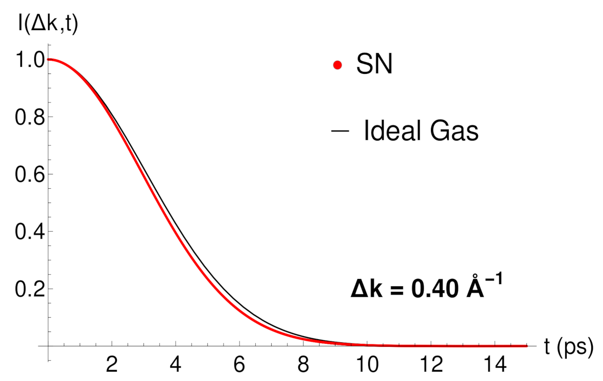
In Figure 1, and in order to first check our propagation method, I ( Δ k x , t ) is plotted versus the propagation time for the surface parallel wave vector transfer Δ k = 0.40 Å 1 , friction coefficient η = 0 , flat potential V = 0 , surface temperature T = 105 K and initial adsorbate velocity v 0 = 115 m/s with negative direction. The propagation time t of the stochastic wave function ψ i ( t ) and the time step Δ t are chosen to be equal to t = 14 ps and Δ t = 0.01 ps, respectively. These values correspond to a number of time steps of N t = 1400 . In Figure 1, our numerical simulation (SN) in red is also plotted showing a very good agreement with the analytic function (43), valid for a 2D ideal gas. This result indicates that the Xe-Pt(111) system under these conditions behave as a true 2D ideal gas where the diffusion of the adsorbate Xe is completely free on the Pt(111) surface. This behavior observed in Figure 1 is also reproduced for different Δ k values in the interval [ 0.05 , 2.5 ] Å 1 analyzed. This free particle motion is kept at very long times.
The next step is now to study the behavior of this system in the ballistic regime at different friction coefficients for a flat surface and compare with experimental results and previous standard Langevin simulations [20]. As mentioned above, this regime is only valid at times t < < η 1 . For such a goal, our purpose is to see how good the Gaussian function, which describes the ballistic regime, is. The Fourier transform in time of the Gaussian ISF is again a Gaussian function which corresponds to the DSF. The full width at half maximum (FWHM) of the SDF, Γ , is extracted and plotted at different frictions for different momentum transfer values Δ k [ 0.05 , 2.5 ] Å 1 . The friction coefficients η used in these simulations are equal to the values used in a previous work [20]. By fitting the ISF to a Gaussian function with width σ t , e x p ( t 2 / 2 σ t ) , the values of Γ can be obtained from σ t through
Γ = 2 2 ln 2 σ t .
The width in time space σ t of the ISF for a 2D ideal gas (43) is σ t = 2 / v 0 Δ k . Using (44), the dependence of Γ with the parallel wave vector transfer Δ k is given by
Γ = 2 ln 2 v 0 Δ k .
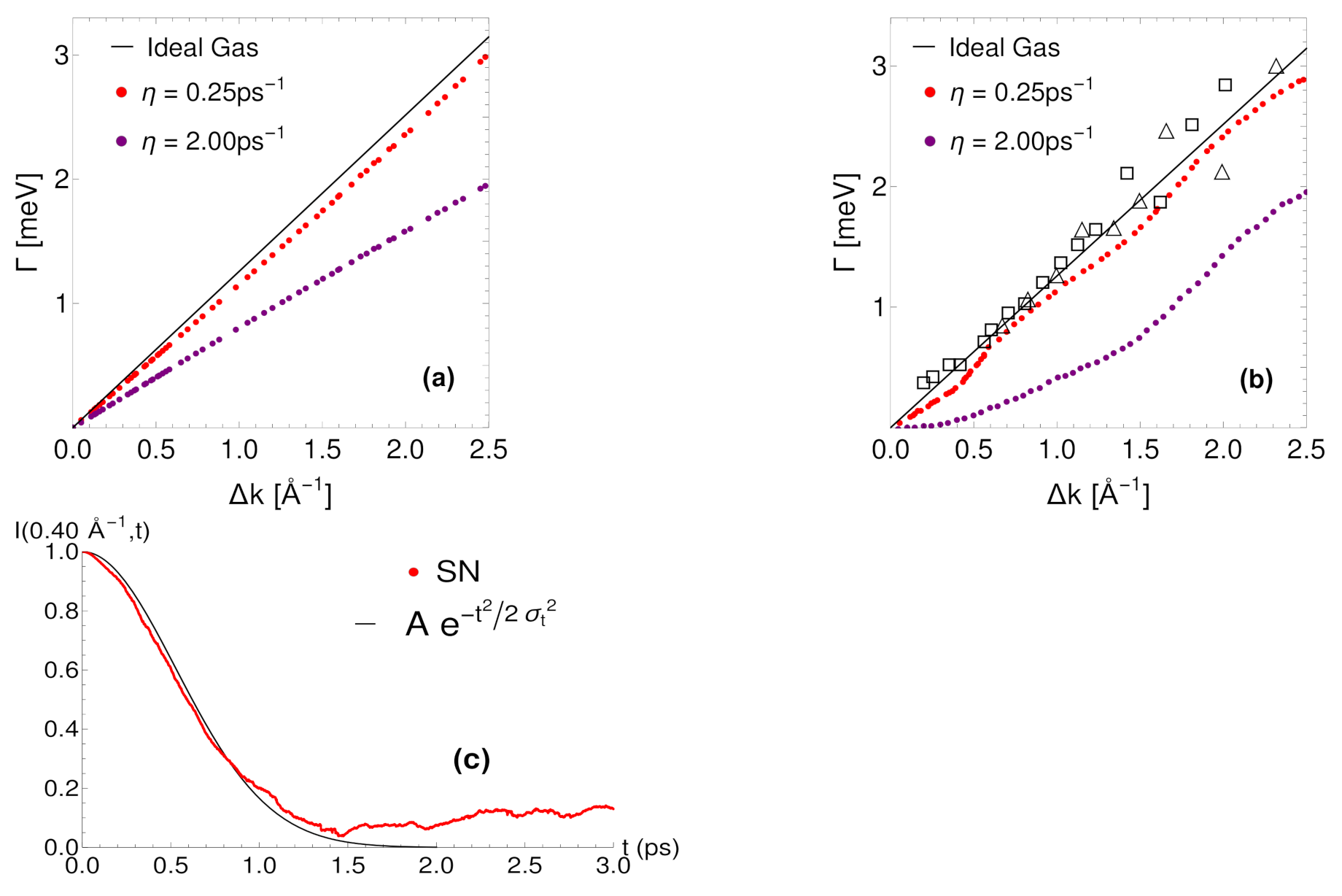
Figure 2 shows a comparison between the numerical results of Γ as a function of the parallel wave vector transfer Δ k at T = 105 K for two different values of the friction coefficient, η = 0.25 , 2.0 ps 1 , and by assuming the corrugation of the Pt(111) surface to be negligible. Black lines correspond to Equation (45). Left top panel (a) displays our numerical simulations. Langevin molecular dynamics simulations are displayed on the right top panel (b) [20] for the same conditions. In panel (c), the fitting to a Gaussian function of the ISF at very short times and small friction is also plotted. The numerical results are in good agreement with those obtained in Ref. [20]. The slope of Γ decreases as the friction coefficient increases. For a fixed value of Δ k , the value of Γ is higher for η = 0.25 ps 1 , so the width in the time domain is smaller and the function I ( Δ k , t ) decays faster. Thus, at higher values of Δ k , the fitting has to be carried out at smaller times. In panel (c), the ballistic regime ( t < < 4 ps) seems to be well described around 0.8 ps. For η = 2.00 ps 1 , the friction is high enough to drastically reduce the ballistic regime at very, very short times. In this case, the interaction with the substrate is very important and the diffusive regime is reached at times t > > η 1 . This regime is not studied here.

3.2. Corrugated Potential

The potential energy surface (PES) is simulated using the pairwise additive potential approximation between the Xe and a square network of Pt atoms with a distance equal to the unit cell length a = 3.93 Å . To ensure that the metal surface is large enough so that the boundary effects do not influence the interaction potential, the number of cells N c of the surface in the X Y plane is increased until the variation in the potential is as small as a given threshold, say 10 3 meV.
A cosine corrugation function is proposed to represent the potential energy surface of the Xe-Pt(111) system given by V a ( x , y ) = V 1 cos 2 π a x cos 2 π a y + V 2 , where V 1 = 13.64 meV and V 2 = 12.32 meV. These values are obtained by fitting the cosine function to the PES numerical result. Both numerical and analytic PSE are very similar because the amplitude of the interaction potential takes an approximated value equal to 28 meV and the periodicity match with the unit cell length of the Pt for both cases. The unidimensional corrugated potential is then used in the simulations with the form V ( x ) = V a ( x , 0 ) = V 0 cos 2 π a x . The amplitude V 0 is taken so that the energy barrier for this potential ( E b = V 0 ) coincides with the Langevin molecular simulations [
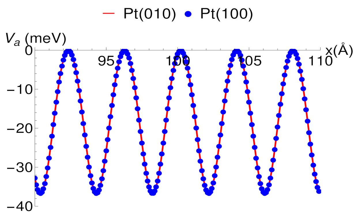
20]. In Figure 3, the directions (010) and (100) of the metallic surface of Pt are plotted for the corrugated potential V a ( 0 , y ) and V a ( x , 0 ) , respectively, in the interval x [ 90 , 110 ] Å . The shape of the potential cutoff along the (010) direction is analogous to the (100). Thus, the diffusion of the Xe adsorbate on the metal surface of Pt is studied using the (100) direction for the interaction potential.
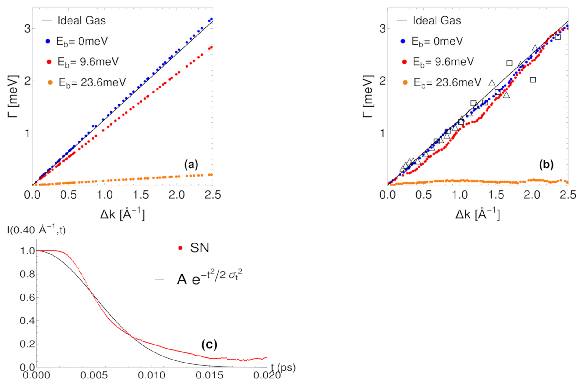
In Figure 4, the influence of surface corrugation on the Xe-Pt(111) system for a simulation with small friction coefficient η = 0.03 ps 1 and surface temperature T = 105 K is analyzed. Figure 4 shows the quasielastic broadening Γ as a function of Δ k . The slope of Γ decreases as E b increases. The adsorbate thermal energy can be obtained from E T = k B T . For a temperature of T = 105 K, the thermal energy is E T = 9.04 meV. If the energy barrier is less than 9.04 meV, the adsorbate can diffuse more or less freely over the metal surface of Pt. For energy barriers belonging to this range, the system is in a ballistic regime at very short times. If E b = 9.6 meV, the difference between both energies is small and the system is at the limit where some Xe gas particles can be trapped, but others can diffuse over the surface. However, if E b > 9.6 meV the thermal energy is not enough to overcome the barrier and almost all the adsorbate particles are trapped in the potential valley and there is no diffusion. In panel (c), the propagation time is much smaller than 1 ps in order to be in the ballisitc regime, t < < η 1 . In this case, the chosen energy barrier is E b = 9.6 meV and the fitting to a Gaussian function is worse. The system under these conditions behaves as a free 2D gas within a unit cell for very short times, particles are trapped inside the potential valley. If a lower barrier energy is chosen, the corresponding fitting is better and the propagation time in this regime is longer. Our numerical results are in good agreement with those obtained by Langevin molecular simulations [20] and experimental data marked by triangles and squares at low E b values.

4. Conclusions

The stochastic wave function formalism has been briefly reviewed and applied to the diffusion of a Xe gas on a Pt(111) surface. The Lindblad master equation, when it is solved by means of stochastic wave functions, provides a good physical description of the ballistic regime in this diffusion process. It provides an efficient numerical scheme to study the quantum dynamics of open systems. As far as we know, this is the first time this theoretical formalism has been applied to the surface diffusion context, since most of works use the Langevin formalism (in its generalized or standard version). This is particularly encouraging since recent experiments with better spatial and time resolutions (HeSE technique) tend to reveal the underlying properties of individual systems and their jump events directly in the time domain. New results for low and moderate values of the surface coverage for the Xe/Pt(111) system have been recently obtained. Thus, thanks to this type of study with quite satisfactory results, the next step will be to extend this theoretical formalism to deal with the diffusion regime, t > > η 1 . This would allow us to consider more physical systems where recent experimental results are waiting for a better interpretation. Adsorbates, such as N a , L i , H 2 , etc., on metallic surfaces have been studied by using the HeSE technique. For light adsorbates, quantum methods are more convenient than classical ones. In the surface diffusion context, this extension, which would be carried out for the first time, is again very promising.

Perspectives

The dependence with the surface temperature and coverage can be studied for a better understanding of microscopic processes. It is suggested to also extend and improve this numerical method for times greater than 20 ps with periodic two-dimensional interaction potential in order to reach the Brownian regime. This method turns out to be a valuable alternative for dealing with more diffusive systems studied via QHAS or HeSE such as, for example, Na-Cu(001), Ar-MgO(100), etc., which have been previously considered within the Langevin formalism [14,18,40].

Author Contributions

E.E.T.-M. carried out the calculations and G.R.-L. supervised her work. E.E.T.-M., G.R.-L., J.R.-S. and S.M.-A. have read and agreed to the published version of the manuscript.

Funding

This research was funded by Ref. FIS2017-83473-C2-1-P (SMA) from the Ministerio de Ciencia, Universidades e Innovación (Spain).

Acknowledgments

This work was partially supported by grants from the Programa Nacional de Ciencias Básicas de Cuba with Ref. No. P223LH001-108 (J.R.-S., and G.R.-L.) and Ref. FIS2017-83473-C2-1-P (SMA) from the Ministerio de Ciencia, Universidades e Innovación (Spain). We thank Angel Sanz for providing us with the original code from which we have made our simulations.

Conflicts of Interest

The authors declare no conflict of interest.

References

  1. Von Neumann, J. Mathematical Foundations of Quantum Mechanics; Princeton University Press: Princeton, NJ, USA, 1955. [Google Scholar]
  2. Gorini, V.; Kossakowski, A.; Sudarshan, E.C.G. Completely positive dynamical semigroups of N-level systems. J. Math. Phys. 1976, 17, 821–825. [Google Scholar] [CrossRef]
  3. Gardiner, C.; Zoeller, P. Quantum Noise; Springer: Berlin/Heidelberg, Germany; New York, NY, USA, 1991. [Google Scholar]
  4. Breuer, H.; Petruccione, F. The Theory of Open Quantum Systems; Oxford University Press on Demand: New York, NY, USA, 2002. [Google Scholar]
  5. Huelga, S.; Huelga, S.F. Open Quantum Systems: An Introduction; Springer: Berlin, Germany, 2012. [Google Scholar]
  6. Langmuir, I. The adsorption of gases on plane surfaces of glass, mica and platinum. J. Am. Chem. Soc. 1918, 40, 1361. [Google Scholar] [CrossRef] [Green Version]
  7. Gao, S.; Busch, D.; Ho, W. Femtosecond dynamics of electron-vibrational heating and desorption. Surf. Sci. 1995, 344, L1252. [Google Scholar] [CrossRef]
  8. Gao, S. Lindblad approach to quantum dynamics of open systems. Phys. Rev. B 1998, 57, 4509. [Google Scholar] [CrossRef]
  9. Droguett, S. Elementos de Catálisis Heterogénea; Oea: South East Queensland, Australia, 1983. [Google Scholar]
  10. Manzi, S.; Costanza, G.; Pereyra, V. Adsorption-desorption kinetics with multiple site occupation. Rev. Mex. Física 2005, 51, 21. [Google Scholar]
  11. Chen, D.; Sarid, D. Temperature effects of adsorption of (C60) molecules on Si(111)-(7×7) surfaces. Phys. Rev. B 1994, 49, 7612. [Google Scholar] [CrossRef]
  12. Karmakar, K.; Maity, D.; Pal, D.; Mandal, K.; Khan, G. Photo-Induced Exciton Dynamics and Broadband Light Harvesting in ZnO Nanorod-Templated Multilayered 2D MoS2/MoO3 Photoanodes for Solar Fuel Generation. ACS Appl. Nano Mater. 2020, 3, 1223–1231. [Google Scholar] [CrossRef]
  13. Miret-Artés, S.; Pollak, E. The dynamics of activated surface diffusion. J. Phys. Condens. Matter 2005, 17, S4133. [Google Scholar] [CrossRef]
  14. Ward, D. A Study of Spin-Echo Lineshapes in Helium Atom Scattering from Adsorbates. Ph.D. Thesis, University of Cambridge, Cambridge, UK, 2013. [Google Scholar]
  15. Tersoff, J.; Hamann, D. Theory of the scanning tunneling microscope. Phys. Rev. B 1985, 31, 805. [Google Scholar] [CrossRef]
  16. Miller, M. Atom probe microanalysis, principles and applications to materials problems. Mater. Res. Soc. 1989. [Google Scholar] [CrossRef]
  17. Celli, V. Theory of Helium Scattering from Surface Phonons. In Surface Phonons; Springer: Berlin, Germany, 1991; p. 191. [Google Scholar]
  18. Casado, R.; Vega, J.; Sanz, A.; Miret-Artés, S. Quasielastic He atom scattering from surfaces: A stochastic description of the dynamics of interacting adsorbates. J. Phys. Condens. Matter 2007, 19, 305002. [Google Scholar] [CrossRef]
  19. Tabony, J.; Perly, B. Quasielastic neutron scattering measurements of fast local translational diffusion of lipid molecules in phospholipid bilayers. Biochim. Biophys. Acta-(BBA)-Biomembr. 1991, 1063, 72. [Google Scholar] [CrossRef]
  20. Ellis, J.; Graham, A.; Toennies, J. Quasielastic helium atom scattering from a two-dimensional gas of Xe atoms on Pt(111). Phys. Rev. Lett. 1999, 82, 5072. [Google Scholar] [CrossRef]
  21. Jardine, A.P.; Alexandrowicz, G.; Hedgeland, H.; Allison, W.; Ellis, J. Studying the microscopic nature of diffusion with helium-3 spin-echo. Phys. Chem. Chem. Phys. 2009, 11, 3355–3374. [Google Scholar] [CrossRef] [PubMed]
  22. Dekker, H.; Valsakumar, M. A fundamental constraint on quantum mechanical diffusion coefficients. Phys. Lett. A 1984, 104, 67. [Google Scholar] [CrossRef]
  23. Caldeira, A.; Leggett, A. Quantum tunneling in a dissipative system. Ann. Phys. 1983, 149, 374. [Google Scholar] [CrossRef]
  24. Jackson, B. Reduced density matrix approach for gas-solid scattering. Chem. Phys. Lett. 1997, 270, 484. [Google Scholar] [CrossRef]
  25. Berman, M.; Kosloff, R.; Tal-Ezer, H. Solution of the time-dependent Liouville-von Neumann equation: Dissipative evolution. J. Phys. Math. Gen. 1992, 25, 1283. [Google Scholar] [CrossRef] [Green Version]
  26. Berman, M.; Kosloff, R. Time-dependent solution of the Liouville-von Neumann equation: Non-dissipative evolution. Comput. Phys. Commun. 1991, 63, 20. [Google Scholar] [CrossRef]
  27. Datta, S. Electronic Transport in Mesoscopic Systems; Cambridge University Press: Cambridge, UK, 1997. [Google Scholar]
  28. Bout, D. Single-molecule studies of heterogeneous dynamics in polymer melts near the glass transition. Science 1997, 277, 1074. [Google Scholar] [CrossRef] [Green Version]
  29. Casado, R.; Vega, J.; Sanz, A.S.; Miret-Artés, S. Quasi-elastic peak lineshapes in adsorbate diffusion on nearly flat surfaces at low coverages: The motional narrowing effect in Xe on Pt (111). J. Phys. Condens. Matter 2007, 19, 176006. [Google Scholar] [CrossRef] [PubMed] [Green Version]
  30. Hove, L.V. Correlations in Space and Time and Born Approximation Scattering in Systems of Interacting Particles. Phys. Rev. 1954, 95, 249. [Google Scholar] [CrossRef] [Green Version]
  31. Vineyard, G. Scattering of slow neutrons by a liquid. Phys. Rev. 1958, 110, 999. [Google Scholar] [CrossRef]
  32. Lovesey, S.; Stephen, W.; Jeffrey, W. Theory of Neutron Scattering from Condensed Matter. Phys. Today 1986, 39, 64. [Google Scholar] [CrossRef]
  33. Diósi, L. Calderia-Leggett master equation and medium temperatures. Phys. A Stat. Mech. Appl. 1993, 199, 517. [Google Scholar] [CrossRef]
  34. Grabert, H.; Schramm, P.; Ingold, G. Quantum Brownian motion: The functional integral approach. Phys. Rep. 1988, 168, 115. [Google Scholar] [CrossRef]
  35. Lindblad, G. On the generators of quantum dynamical semigroups. Commun. Math. Phys. 1976, 48, 119–130. [Google Scholar] [CrossRef]
  36. Kossakowski, A. On quantum statistical mechanics of non-Hamiltonian systems. Rep. Math. Phys. 1972, 3, 247. [Google Scholar] [CrossRef]
  37. Dekker, H.; Valsakumar, M. Identification of possible contamination sources using reverse hydraulic simulation. Phys. Lett. 1984, 104A, 67. [Google Scholar] [CrossRef]
  38. Gao, S. Dissipative quantum dynamics with a Lindblad functional. Phys. Rev. Lett. 1997, 79, 3101. [Google Scholar] [CrossRef]
  39. Gisin, N.; Percival, I. The quantum-state diffusion model applied to open systems. J. Phys. A Math. Gen. 1992, 25, 5677. [Google Scholar] [CrossRef]
  40. Mantecón, J.; Miret-Artés, S.; Rojas-Lorenzo, G. Diffusion of Ar Atoms on MgO (100) Surfaces. Rev. Cuba. Física 2012, 29, 8–13. [Google Scholar]
Figure 1. Intermediate scattering function (41) plotted versus the simulation time t ( p s ) for a parallel wave vector transfer Δ k = 0.40 Å 1 , friction coefficient η = 0 , surface temperature T = 105 K and inital adsorbate velocity v 0 = 115 m/s with negative direction. The red curve corresponds to the numerical results of our simulations (SN) and the black curve to the Gaussian function (43).
Mathematics 09 00362 g001
Figure 2. Quasielastic broadening Γ from Equation (44) as a function of surface parallel wave vector transfer Δ k x for the decay process of the function I ( Δ k , t ) with a low coverage θ = 0.017 , surface temperature T = 105 K and initial adsorbate velocity v 0 = 115 m/s. Black lines correspond to Equation (45). (a) Numerical simulations for a flat surface ( V = 0 meV) with friction coefficients η = 0.25 ps 1 (red) and η = 2.0 ps 1 (purple). (b) Langevin molecular dynamics simulations from Ellis et al. [20]. Experimental results from the QHAS broadening at two incident He beam energies E i = 10.15 meV (triangles) and E i = 26.85 meV (squares). (c) The ISF given by Equation (41) is plotted versus the simulation time in ps for Δ k = 0.40 Å 1 and friction coefficient η = 0.25 ps 1 . Our simulation results (SN) are represented by the red curve and the fitting Gaussian function e t 2 / 2 σ t 2 by the black curve.
Mathematics 09 00362 g002
Figure 3. Projections of the interaction potential V a along the directions (100) and (010) of the surface in the interval x [ 90 , 110 ] Å . The projection on the (010) direction is represented by a red curve and the projection on (100) has been represented by blue points.
Mathematics 09 00362 g003
Figure 4. Quasielastic ( Γ ) broadening as a function of Δ k with a low coverage ( θ = 0.017 ), small friction coefficient η = 0.03 ps 1 , surface temperature T = 105 K and the initial adsorbate velocity v 0 = 115 m/s. (a) Results of the simulations for potential energy barrier: E b = 0 meV (blue), E b = 9.6 meV (red) and E b = 23.6 meV (orange). (b) Results of a Langevin molecular dynamics taken from Ellis et al. [20] with the same values of the energy barrier mentioned before, the theoretical result for a 2D ideal gas (45) and experimental results of the QHAS broadening for two incident beam energies E i (triangles, E i = 10.15 meV; squares, E i = 26.85 meV) for scattering from Xe adsorbed on a Pt(111). (c) The ISF I ( 0.40 Å 1 , t ) versus the simulation time t(ps) for an energy barrier E b = 9.6 meV. Our simulation (SN) is represented by a red curve and the Gaussian function e t 2 / 2 σ t 2 by a black curve.
Mathematics 09 00362 g004
Publisher’s Note: MDPI stays neutral with regard to jurisdictional claims in published maps and institutional affiliations.

