Article

Path-Planning for Mobile Robots Using a Novel Variable-Length Differential Evolution Variant

by
Alejandro Rodríguez-Molina
1,*,
José Solís-Romero
1,
Miguel Gabriel Villarreal-Cervantes
2,*,
Omar Serrano-Pérez
2 and
Geovanni Flores-Caballero
2
1
Tecnológico Nacional de México/IT de Tlalnepantla, Research and Postgraduate Division, Estado de México 54070, Mexico
2
Postgraduate Department, Instituto Politécnico Nacional, CIDETEC, Mexico City 07700, Mexico
*
Authors to whom correspondence should be addressed.
Mathematics 2021, 9(4), 357; https://doi.org/10.3390/math9040357
Submission received: 21 January 2021 / Revised: 5 February 2021 / Accepted: 7 February 2021 / Published: 11 February 2021
(This article belongs to the Special Issue Fuzzy Sets and Soft Computing)

Abstract

:
Mobile robots are currently exploited in various applications to enhance efficiency and reduce risks in hard activities for humans. The high autonomy in those systems is strongly related to the path-planning task. The path-planning problem is complex and requires in its formulation the adjustment of path elements that take the mobile robot from a start point to a target one at the lowest cost. Nevertheless, the identity or the number of the path elements to be adjusted is unknown; therefore, the human decision is necessary to determine this information reducing autonomy. Due to the above, this work conceives the path-planning as a Variable-Length-Vector optimization problem (VLV-OP) where both the number of variables (path elements) and their values must be determined. For this, a novel variant of Differential Evolution for Variable-Length-Vector optimization named VLV-DE is proposed to handle the path-planning VLV-OP for mobile robots. VLV-DE uses a population with solution vectors of different sizes adapted through a normalization procedure to allow interactions and determine the alternatives that better fit the problem. The effectiveness of this proposal is shown through the solution of the path-planning problem in complex scenarios. The results are contrasted with the well-known A* and the RRT*-Smart path-planning methods.

1. Introduction

1.1. A Review of Path-Planning Methods

Robots have become fundamental tools to perform diverse activities, mainly those that are dangerous or tough for humans [1]. Particularly, mobile robots extend the operation of classical fixed-base robotic manipulators to almost any place [2].
The success of mobile robots depends on their autonomy degree, i.e., insofar as they require less human intervention [3]. Among the tasks required to achieve autonomy in robots, path-planning is one of the most critical [4].
Without loss of generality, the path-planing problem is to find a sequence of path elements (points, curves, line segments, etc.) that connect a start point to a target one avoiding threats (usually, collisions with obstacles or risky regions) and achieving the best performance (typically, the shortest length) [5]. Since the path’s shape is strongly related to the optimization of energy consumption, the robot’s safety, navigation time and the path’s overall cost [6], the relevance of the path-planning task is highlighted.
In the last decades, several path-planning solution approaches, also named path-planners, have been proposed and can be classified in five categories [7]: (i) sampling-based algorithms, (ii) node-based optimal algorithms, (iii) mathematical-model-based algorithms, (iv) bio-inspired algorithms and (v) multifusion-based algorithms.
The path-planners in (i) randomly or heuristically sample the path elements to find a feasible and short path. Within this category, the Rapidly-exploring Random Trees (RRT) [8], and the Probabilistic Road Maps (PRM) [9] stand out. In RRT, random points in the workspace are incrementally sampled in a radius to generate branched feasible path segments. Therefore, the resulting tree contains the searched path. On the other hand, the PRM samples random nodes in a radius within the workspace and creates collision-free connections among them. After this, PRM selects a feasible path between the start and target nodes. Despite the rapid exploration of the workspace with RRT and PRM, the probability of finding the shortest path is extremely low [10]. Improved RRT and PRM versions like RRT* and PRM* have been proposed to obtain the shortest possible path by taking into account each branch length and scaling the sampling radius gradually, respectively [11]. The main shortcoming of the methods in (i) is that calculating the best path depends on probability, while their main strength is the computational efficiency. Moreover, a human intervention must establish the proper sampling radius and the number of sampled points or branches, affecting the robot autonomy. If the above parameters are settling incorrectly, it may result in a very low-performance path or excessive calculation time.
Category (ii) includes techniques that require the workspace to be described in a graph. These techniques then explore the graph to find the shortest path between the start and target nodes, usually as variants of the Dijkstra algorithm. Four representative methods are the A* [12], the Fast Marching (FM) [13], the Potential Field (PF) [14] and the Visibility Graphs (VG) [15]. A* is a greedy and deterministic technique that heuristically finds sub-optimal paths in informed graphs. A well-known variant of A* is the D* that deals with dynamical workspaces [16]. FM solves a discretized version of the Eikonal wave propagation differential equation in a graph. The solution to this equation is related to the wave’s arrival time at each node in the graph from a given origin node. The propagation of the wave generates a velocity field at each node used to calculate the arrival times to its neighbors. The best route is the one that takes the wave from the origin to the destination in the shortest cumulative time, and is obtained by the gradient descent. The PF method applies a potential field to the workspace. This field generates an attractive force between any node in the graph and the target, and induces a repulsive effect to the obstacles or risky regions. Based on the above two effects, a potential can be calculated for each node. Then, the best path can be found as the lowest cumulative potential alternative through the gradient descent. In VG, the vertices of each obstacle in the workspace are selected as the nodes of a graph, and the connections among them are established based on visibility, i.e., a collision-free edge between each pair of nodes. The best path is obtained from that graph. Since all the above methods discretize the workspace, their effectiveness depends on how the graph is built. The most accurate workspace representation requires an infinite graph of which the best path cannot be found in finite time. In practice, the human establishes a proper trade-off between planning precision and computational cost. If each node in the graph represents a wide region of the workspace, the obtained path may be very long, but the calculation could be fast. The opposite can happen if each node is associated with a smaller region.
The methods in (iii) require an accurate mathematical model of the workspace and the mobile robot. Based on that model, a linear or non-linear dynamic programming problem is established to find the control actions that take the robot through the best feasible path. The above problem, also known as the optimal control problem, is typically solved by classical direct or indirect methods. The work in [17] shows a clear example of this category. In that proposal, a dynamic control problem is solved in the path-planning for a spherical mobile robot. Although the methods in (iii) can achieve the lower cost path theoretically, their performance is limited by model accuracy. All models are imprecise, and the above coupled with the presence of uncertainties and disturbances [18] in the real-world can lead to poor performance in path-planning.
The bio-inspired approaches in (iv) use analogies with biological or physical phenomena to solve the path-planning problem. In this sense, Artificial Intelligence (AI) techniques such as Fuzzy Logic (FL), Neural Networks (NNs) and meta-heuristics are recurrently found in the specialized literature. In [19], the Ant Colony Optimization (ACO) algorithm improved with FL is used to obtain cost-effective paths with an unmanned aerial vehicle in dynamic environments. Another example is the work in [20], where a NN is used to dynamically predict and avoid collisions in the path-planning for mobile robots. On the other side, the meta-heuristic approaches are referred to as algorithms from evolutionary computation and swarm intelligence that solve a formal optimization problem to find the path elements that minimize its overall cost. These methods are discussed further in this document. The methods in (iv) have shown outstanding performance, especially when the path-planning problem is hard, e.g., when there are moving obstacles or the path cost involves other criteria beyond the overall length such as energy, time, shape, etc. Nevertheless, the computational cost of these methods can be considered higher than the previous categories. Particularly, the FL and NN methods need proper training to generalize an expert human’s knowledge before its use.
Finally, the techniques in (v) combine different features of the other four categories. The above aims to enhance the path-planning effectiveness by decreasing the implicit drawbacks of a single category. An example of these techniques is found in [21]. In the above research, an NN improves the RRT* algorithm by determining a suitable sampling distribution.

1.2. Optimization in Path-Planning

Optimization is required in almost every engineering application due to the current limitations and challenges of modern life, and path-planning is not an exception. It is used either to reduce costs [22], improve accuracy [23], raise the incomes [24] or enhance other performance indicators. The systematic procedure in the general optimization process for engineering is noticeable. First, the system or process is studied in-depth to determine the relationships among the involved variables (design variables), the performance needs (objectives) and the overall limitations (constraints). The above elements are established, through the mathematical language, as a formal optimization problem. Finally, an optimizer is used to find suitable solutions that can be implanted in the final application. Therefore, the path-planning problem can be formally stated as an optimization problem, where the path requirements can be expressed as the objectives, the path elements are the design variables and the constraints can be set to prevent risky behaviors [25]. By its own nature, the path-planning optimization problem is Non-Polynomial Hard (NP-Hard) one [26], and deterministic optimization techniques may not achieve the best performance. Fortunately, the use of soft computing techniques such as meta-heuristics has shown outstanding results compared to deterministic solution methods and state-of-the-art sampling and node-based approaches [25,27]. In this sense, meta-heuristics are stochastic computational techniques that can find good solutions to complex optimization problems using a reasonable amount of resources [28]. Those based on evolutionary computation and swarm intelligence stand out among meta-heuristic methods.
On the other hand, for a wide variety of optimization problems associated with real-world applications, the engineer knows the variables involved in the process or system, which must be adjusted to optimize the outcome. Nevertheless, there are more intricate problems where the identity or the number of the involved variables is uncertain [29]. Examples of the above problems are observed in controller design [30], re-configurable robotics [31], machine scheduling [32], among others.
Path-planning for mobile robots is part of the problems described in the previous paragraph since the number of path elements cannot be known a priori. A common way to address this issue requires human intervention to propose or decide the number of path elements (points in the Cartesian plane) to be adjusted. For example, an improvement of the Particle Swarm Optimization (PSO) is proposed in [33] to optimize a mobile robot’s trajectory. PSO can place the points that the robot travels in each iteration, solving an optimization problem that considers the distance to the target point and the obstacles’ separation. The proposal in [34] introduces a new crossing operator in the GA to optimize the location of the points that make up a trajectory for mobile robots. GA uses a cost function that considers the total distance, the robot’s energy and the safety of the path. In [35], a method is proposed to find the point local positions of a trajectory sequentially (points that the robot travels from an initial location to a final one) through the Differential Evolution (DE) algorithm. The method finds a new feasible point position on each iteration to minimize the distance to an end point. The work in [36] presents a hybridization between PSO and DE to solve the problem of trajectory planning for mobile robots. The problem aims to minimize a single target that considers the total distance and the trajectory’s safety. The trajectory is made up of consecutive points located over vertical lines of action within the Cartesian space. The research in [37] proposes a hybridization between a GA and the A* planning technique to find the spline segments of a trajectory for the differential wheeled robot. An optimization problem is formulated that weights four objectives, the distance, the travel time, the smoothness and the safety of the trajectory (based on how close the mobile robot passes to the obstacles).
It can be observed that the main drawback of the above approach is the reduction of autonomy in mobile robots, i.e., mobile robots cannot decide the number of path elements by themselves and the human help is needed. Additionally, if the number of path elements is not well established, a large value can over-define the path (this can complicate the post-processing task aspects [38] such as path smoothing [39], control [40]) and energetic efficiency [41], while a lower one can reduce the chances of finding the optimal path [42]. A way to deal with the above difficulty is to treat the path-planning as a Variable-Length-Vector Optimization Problem (VLV-OP) to determine the number of the variables (points) and their values (Cartesian coordinates) enhancing the application performance. The above implies an additional complexity in the problem, and its solution requires more sophisticated optimization mechanisms, even in the meta-heuristics.
To the best of the author’s knowledge, the path-planning as a VLV-OP has been investigated little. In this way, two representative works [43,44] can be found in the specialized literature. Both alternatives take advantage of the GA’s binary encoding to deal with the VLV-OP in discrete workspaces modeled as finite grids. In [43], the GA with a simple one-point crossover, a swap mutation and a gene elimination mechanism is adopted to evolve the generation of mobile robots’ paths. On the other hand, the work in [44] finds optimal trajectories for a robotic manipulator using the GA. The adopted one-point crossover uses information regarding nodes’ location in two paths to select the split point. Simultaneously, the mutation strategy alters random points on the path based on the location of its neighbors.
Although only a couple of works address the path-planning problem as a VLV-OP, different solution approaches can be found from other application contexts. For example, GAs are also proposed to solve VLV-OPs related to the preventive maintenance scheduling problem [45], the headway optimization and the scheduling combination problem for vehicles [46] and the routing problem for informed graphs [47,48]. Those works require fewer modifications of the GAs to solve VLV-OPs, and their effectiveness is limited to discrete search spaces.In the case of path-planning problems, discrete workspaces reduce the accuracy of the found paths in the sense that optimizers cannot find the optimal solution [25]. However, variations of well-known meta-heuristic optimizers such as DE and PSO have been proposed to solve VLV-OPs in engineering with continuous search spaces. Related to DE, the work in [49] proposes a DE variant to solve the satellite re-configuration problem using a fixed-length vector alongside an expression vector that determines the activation of a chromosome. A similar approach is found in [50], where DE was used for clustering. In this DE variant, the chromosome is divided into activation genes (threshold to decide which centroid is active) and genes that include the cluster centroids. Since the vector size remains fixed for all solutions, classical DE operators are used by their own nature. In the operational amplifier design, circuit components are represented by blocks with a variable number of genes into a fixed-length vector, where unusable genes are set to zero in [51]. To allow the use of classical DE operators, truncation and expansion procedures are adopted to standardize chromosomes’ size. In PSO to solve VLV-OPs, some applications with continuous search spaces have also been developed. In [52], the maintenance scheduling problem for a pressurized water reactor is solved by a PSO variant. The particles represent variable groups of interventions on maintenance days. The particle information is included in a fixed-length vector, where a variable equal to or lower than zero denotes a state of non-activation. Then, the traditional PSO operators can be applied without additional considerations. Relevant applications of PSO for VLV-OPs are also related to the optimization of neural networks. In [53], PSO optimizes the layers of convolutional neural networks. It uses a fixed-length vector with binary encoding and a range of variable values to represent a disabled state of a layer. On the other hand, the work published in [54] uses PSO to automatically select the number of hidden neurons, the input weights and the hidden biases in a single hidden layer feedforward. A stochastic strategy was proposed to update particle sizes and apply the original PSO operators over actual variable-length solutions to achieve it. In the case of DE and PSO to solve VLV-OPs in engineering with continuous search spaces, most of the alternatives found in literature use a fixed-vector to represent individuals or particles and strategies to distinguish the active variables (i.e., those variables that are considered in the problem evaluation). For techniques with actual variable-length-vectors, the previously mentioned strategies aim to stochastically standardize the size of the vectors to apply traditional meta-heuristic operators. However, the above ways to handle VLV-OPs with continuous search spaces may not provide relevant information for the search, i.e., they do not consider the variable values of the current solution alternatives for the standardization.

1.3. Scope and Contributions of the Proposal

In this work, the path-planning for mobile robots is conceived as a VLV-OP where the number of path points and their locations must be determined simultaneously to minimize the overall path length. The VLV-OP is established considering the features of a four mecanum wheeled omnidirectional mobile robot and can be easily scaled to other kinds of mobile systems.
The VLV-OP aims to adjust a variable number of sequential path points in a continuous workspace to minimize the total length between the start and target points. In order to avoid collisions with obstacles, a hard equality constraint is imposed on the VLV-OP. In this way, a path is assigned to a simple 2D shape to ensure the robot safety in the path tracking, and obstacles are treated as polygons to support the collision detection. The above VLV-OP is then solved by a novel variant of Differential Evolution for Variable-Length-Vector optimization (VLV-DE). This optimizer uses an initial VLV population generated by the weighted variant of the A* path-planning method [55] to speed up the finding of the first set of feasible paths. The candidate solution vectors of different sizes are then adapted through a normalization procedure to allow interactions with the ordinary DE operators, i.e., scaling and recombination. This normalization can increase or decrease the vector length by incorporating valuable solution information from the current vector variables. The above helps to generate improved paths that better fit the problem.
For instance, the proposal’s effectiveness is shown through the solution of the path-planning problem in three complex scenarios with different obstacle distributions and shapes. The results are contrasted with those of the original A* method and the RRT*-Smart technique.
The rest of the present work is organized as follows. Section 2 presents the general VLV-OP and introduces the path-planning problem for mobile robots. Section 3 details the operation of the proposed VLV-DE. The experiment details and results are described in Section 4 to show the effectiveness of the proposal. Finally, Section 5 draws some conclusions.

2. The Path-Planning Problem

2.1. General Variable-Length-Vector Optimization Problem

The general Variable-Length-Vector Optimization Problem (VLV-OP) shown in (1), is to find a VLV x of design variables (variables involved in a process or system) that minimizes the value of the objective function J (an indicator of the process or system performance). Unlike classical global optimization problems, where only the value of the design variables in x is searched, the VLV-OP additionally requires the number of design variables to be found, i.e., the size of x, denoted by s ( x ) , is unknown. Moreover, the search space can be delimited by a set of n g inequality constraints g i ( x ) or n h equality constraints h j ( x ) (both usually describe the process or system limitations regarding the cost, space, resources, to name just a few) that describe the feasible search space Ω R s ( x ) . In addition, the box constraints described by x k m i n and x k m a x , can be considered to limit the possible values that each design variable x k can take, while the constraints over s ( x ) control the size of the vector x.
min x Ω J ( x ) subject to : g i ( x ) 0 , i = 1 , , n g h j ( x ) = 0 , j = 1 , , n h x k m i n x k x k m a x , k = 1 , , s ( x ) L m i n s ( x ) L m a x

2.2. The Path-Planning for Mobile Robots as a Variable-Length-Vector Optimization Problem

The path-planing problem for mobile robots is to find the shortest way (a set of consecutive control points p l ) from a start point p s to a target one p t within the workspace W. The workspace W is considered as a finite subspace of R 2 . In this case, W is related to the plane’s coordinates where the mobile robot is placed. Additionally, W includes a set of obstacles or threats. Hence, the obtained path must somehow ensure collision avoidance between the mobile robot and the obstacle geometries.
In this work, the four mecanum wheeled mobile robot (4MWMR) is used to illustrate the development of the path-planning problem. Nevertheless, it can be intuitively extrapolated to other mobile configurations.
The 4MWMR is an omnidirectional mobile robot whose wheels are independently controlled by DC motors. Each wheel includes a single hub circumference, which is circumferentially coupled with a series of rollers oriented at 45 concerning it. A remarkable feature of the 4MWMR is its capability to track nonlinear paths by keeping a constant orientation [56].
The above path-planning problem is put in the form of the general variable-length-vector optimization problem in (1), and its elements are detailed as follows:

2.2.1. The Variable-Length-Vector of Design Variables

The variable-length-vector x in (2) includes the information (2D Cartesian coordinates) of the control points p l , l = 1 , , s ( x ) in the path, i.e., the ordered sequence of positional configurations that the mobile robot must track to reach p t from p s .
x = [ p 1 , , p s ( x ) ] T

2.2.2. The Objective Function

The objective function J in (3) measures the total path length, i.e., the sum of the Euclidean distance (denoted by d e ) of each pair of consecutive points in the path (start point p s , target point p t and control points p l , included) as observed in Figure 1.
J ( x ) = d e ( p s , p 1 ) + l = 1 s ( x ) 1 d e ( p l , p l + 1 ) + d e ( p d , p t )

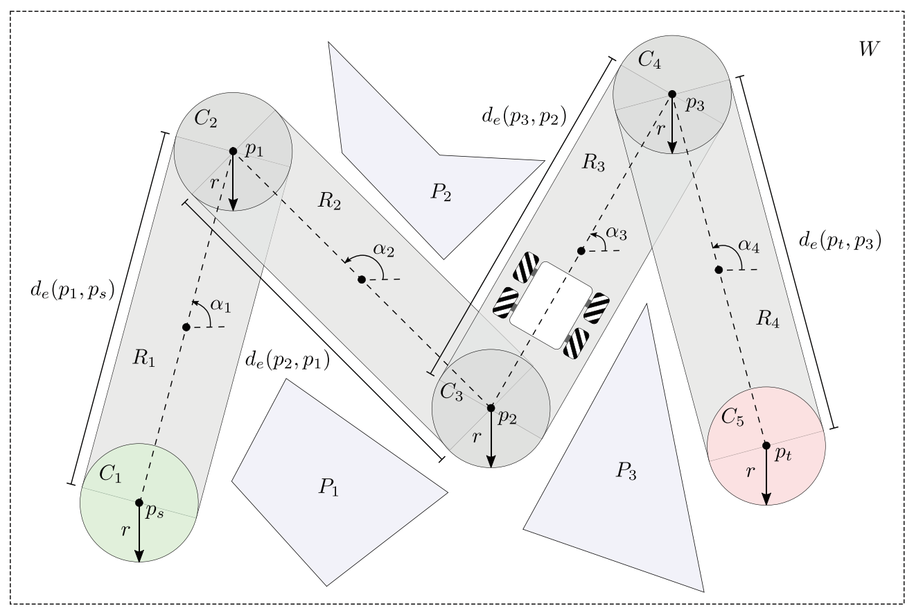
2.2.3. The Constraints

The studied path-planning problem does not consider any inequality constraint but only one equality constraint. The latter is established to strictly avoid the collisions of the mobile robot geometry with the obstacles in W.
In practice, objects of complex geometries are represented by simpler shapes (e.g., boxes, circles, polygons, etc.). The use of these shapes notably improves the computational algorithms’ performance for collision detection [57]. For the above reason, 2D shapes were assigned to all the elements in W, as shown in Figure 1. These shapes are described next:
  • Obstacles: Polygons P m , m = 1 , , n o , defined by an arbitrary number of vertices which describe all the n o obstacles in the workspace W.
  • Path points: Circles C l , l = 1 , , s ( x ) are assigned to each control point in the path. Each circle is centered in the control point and has a diameter of 2 r that matches the length of the longest diagonal of the 4MWMR in the plane. This shape is selected to allow possible orientation changes of the 4MWMR.
  • Path edges: In order to improve the collision detection procedure, rectangular geometries R l , l = 1 , , s ( x ) + 1 are attached to each edge in the path. An edge is the line segment between a pair of consecutive points in the path. The width of each R l is equal to the edge length, its height is 2 r and its orientation matches the inclination α , l = 1 , , s ( x ) + 1 of the edge. The R l is centered in the middle of the two points.
Once the elements in W are assigned to a 2D shape, it is possible to determine if the path geometry (this includes the C l and R l geometries) collides with the ones of the obstacles (the polygons P m ). For this reason, the function (4) implements a polygon-polygon and a polygon-circle collision detection based on the Separating Axis Theorem (SAT) [58,59]. Based on (4), the single equality constraint for the path-planning problem is established in (5), which indicates the times the elements on the path collide with the obstacles in W.
c ( G 1 , G 2 ) = 1 , if G 1 collides G 2 0 , otherwise
h ( x ) = m = 1 n o l = 1 s ( x ) c ( P m , C l ) + m = 1 n o l = 1 s ( x ) + 1 c ( P m , R l )
Additionally, all the control points p l must be inside W. The above conform to the box constraints of the problem. It is important to remark that the VLV-OP for path-planning has particular features distinguishing it from other specialized literature problems. In this sense, all variables are of the same type (2D points), and their position within the VLV of design variables is relevant. The above two features are taken into account while designing the novel optimizer in the next section.

3. The Novel Variable-Length-Vector Differential Evolution

Differential Evolution (DE) is a well-known evolutionary algorithm that has been successfully used to find outstanding solutions to global optimization problems [60]. Moreover, DE has proven to be particularly effective when these optimization problems are related to engineering applications [61].
DE uses an evolutionary procedure over a population (a set of candidate solutions) to explore (i.e., to find potentially good search regions) and exploit (i.e., to obtain outstanding solutions within a search region) the search space towards the global solution [62]. The individuals in the population are initially random, and during a given number of generations, they are recombined and mutated to generate an offspring population. By the end of each generation, the original and offspring populations’ individuals compete to determine those solutions that survive for the next generation. The best solution is found in the population of the last generation. Several variants of DE have been proposed over time, and they differ in the type of used evolutionary operators that improve its explorative and exploitative capacity [63].
The proposed Variable-Length-Vector Differential Evolution (VLV-DE) introduces a novel normalization procedure that allows the interaction of variable-length solutions through the original DE evolutionary operators (mutation, crossover and selection designed for searching in continuous spaces) to solve the VLV-OP associated with the path-planning task for mobile robots.
The above normalization aims to incorporate as much relevant information as possible of a given solution (candidate path) to increase or decrease its number of variables (path nodes).
Unlike the optimizers for continuous VLV-OPs found in the specialized literature, the proposed VLV-DE handles actual variable-length solutions. The above implies the representation of solutions through the use of actual variable-length-vectors.
The operation of the proposed VLV-DE is described in Algorithm 1 and is based on the DE/best/1/bin variant [63]. Nevertheless, it can be easily extended to other DE variants.
The elements of VLV-DE are detailed as follows:
Algorithm 1: Variable-Length-Vector Differential Evolution (VLV-DE)
Mathematics 09 00357 i001

3.1. Initialization

In the first step, as in any DE variant, N P individuals in the population X are randomly generated within the search space (the box constraints given by x k m i n and x k m a x in (1) delimit this space).
Due to the complexity of the path-planning problem, it is improbable to generate a feasible solution during the random initialization. Depending on the workspace conditions and the problem complexity (i.e., the number, location and size of obstacles), it could take several generations to find a feasible solution through the evolutionary process, and even it may never be found.
To address the above difficulty, the weighted A* search algorithm [55] is used to generate a feasible initial population in VLV-DE with different variable-length paths. The weighted variant of A* establishes a trade-off between search performance and computational cost through the weighting factor w [64]. With the larger w, the performance increases, as does the cost, while the opposite happens when w is decremented. The adopted A* uses a grid discretization of the workspace with a cell width and height equal to 2 r (to fit the mobile robot dimension), the Manhattan heuristic model [65], the cost function f ( n ) = 1 + h ( n ) + w ( g ( n ) 1 ) and a uniformly distributed weight w in [ 0 , 1 ] to generate different sub-optimal paths.
Once X is generated, the fitness of each individual is determined by calculating the values J, g i and h j in (1).

3.2. Evolutionary Cycle

During a maximum of G m a x generations, the individuals in X interact to generate mutants. Then, these mutants are recombined with the original individuals in X to obtain offsprings. Finally, the offsprings compete with the individuals in X based on their fitness, and the fittest alternatives persist in X for the next generation.

3.3. Normalization

DE/best/1/bin requires three different individuals x r 1 , x r 2 and x b , to generate a single mutant v i . The individuals x r 1 and x r 2 are randomly selected from the current population X for each solution x i . On the other hand, x b is selected as the fittest solution in X at the start of the current generation. Moreover, DE/best/1/bin uses the mutant v i along with an original individual x i to create an offspring u i .
Computation of both individuals v i and u i is performed through evolutionary operators that require the base solutions (i.e., x i , x r 1 , x r 2 and x b ) to be the same size.
Nevertheless, VLV-DE conceives a population X with individuals of different sizes to solve the VLV-OP in (1), and a normalization procedure needs to be performed to allow interactions by applying the original evolutionary operators of DE/best/1/bin (mutation and crossover).
The normalization procedure, described in Algorithm 2, temporarily adjusts the size of an arbitrary solution to a given value N s . The value of N s is first randomly selected from s ( x i ) , s ( x r 1 ) , s ( x r 2 ) , s ( x b ) to favor the similarity of the generated mutant or offspring with at least one of the involved solutions, i.e., to enhance the exploitation capability of VLV-DE regarding the vector size. Next, the exploration is improved by applying a variation operator to N s . The Gaussian mutation [66] is adopted for this purpose.
If the size of a given solution is greater than N s , its variables must be compressed to obtain an individual of reduced size. On the contrary, if this size is smaller than N s , a decompression procedure is used to increase the original individual size.
Algorithm 2: Normalize
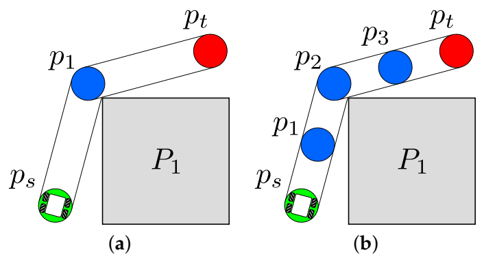
 ( x k , N s )
Mathematics 09 00357 i002

3.4. Compression

This procedure is observed in Algorithm 3 and aims to iteratively reduce the size of an arbitrary individual while losing as little path information as possible. For each iteration, the compression procedure can reduce the size of the individual x k in two ways based on probability:
  • Selecting a pair of consecutive path points and replacing them with a new single one that preserves information from both. The new variable is obtained as the pair’s mean and can be altered through a variation operator (the polynomial mutation [67]) to enhance the exploitative search.
  • Removing the first or the last path point.
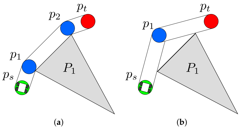
The compression stops once the individual size reaches N s .

3.5. Decompression

Unlike compression, the procedure described in Algorithm 4 aims to iteratively include new valuable variables in the individual to increase its size. As long as the individual size is different from N s , the decompression procedure can increase the size of the individual x k in two ways based on probability:
  • Selecting a pair of consecutive path points to generate a single one based on their information, which is then inserted in the middle of both. This new variable is calculated as the pair’s mean and can be modified by using a variation operator (the polynomial mutation) to improve the exploratory search.
  • Including altered versions of the first or the last path points (obtained through the polynomial mutation), at the beginning or the end of the solution, respectively.
Algorithm 3: Compress ( x k , N s )
Mathematics 09 00357 i003
Algorithm 4: Decompress ( x k , N s )
Mathematics 09 00357 i004

3.6. Evolutionary Operators

At this point, all the individuals required for mutation and crossover have acquired the temporarily forms x i n , x r 1 n , x r 2 n and x b n , which have the same size. Then, the evolutionary operators of the original variant DE/best/1/bin can be applied as usual to generate interactions between individuals. These operators include the mutation in (6), with the scaling factor F [ 0 , 1 ] , and the crossover in (7), with the crossover rate C R [ 0 , 1 ] .
v i = x b n + F · ( x r 1 n x r 2 n )
u i , j = v i , j , if   r a n d ( 0 , 1 ) C R   or   j = j r a n d x i , j n , otherwise

3.7. Selection

At the end of each generation, every individual x i from X is compared to its corresponding offspring u i regarding their fitness. Then, the fittest alternative persists in X for the next generation. Any individual’s fitness considers two important aspects: The compliance with restrictions and the value of the objective function. Due to the above, the binary tournament selection operator in [68] is used to determine the fittest individual by pondering first the feasibility and then the convergence.
When the last generation ends, the best individual is selected as the fittest one in X. This solution can then be implanted in the motion planner for the mobile robot.

3.8. Local Search

An additional local search procedure, shown in Algorithm 5, is applied to all solutions in X to improve their fitness at the end of each generation. This procedure generates a new local solution by altering the size (using Gaussian mutation over the original size and performing the normalization) and the variables (using the polynomial mutation) of the original solution x i . The new solution is compared to the original one to determine the local best alternative.
Algorithm 5: LocalSearch ( x i )
Input: x i (arbitrary solution)
Output: x i l (local best solution)
1  N s s ( x i ) ;
2 Variate N s using Gaussian mutation;
3  x i n Normalize( x i , N s );
4 Variate x i n using Polynomial Mutation;
5 Evaluate x i n ;
6 Select x i l as the best between x i and x i n

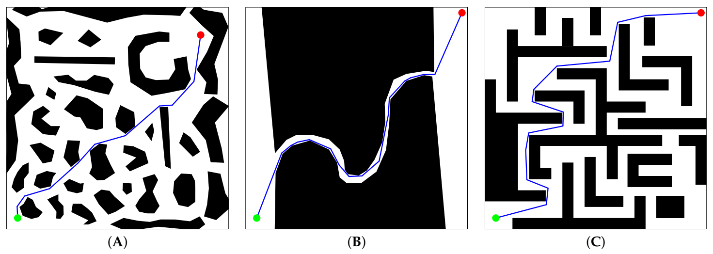
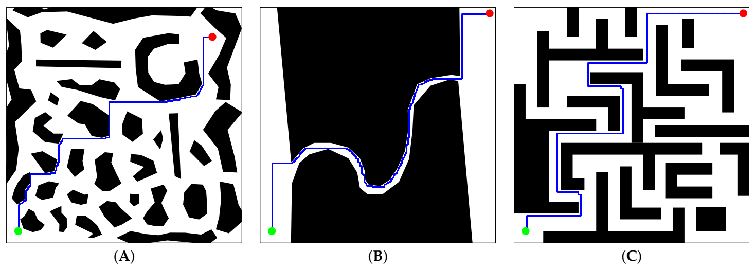
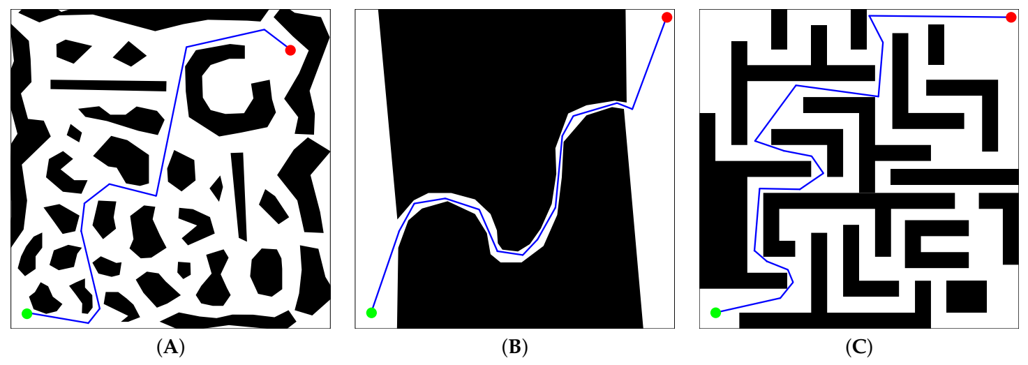
4. Results an Discussion

4.1. Details of the Experiment

Three test cases, (A), (B) and (C), based on the scenarios (Scenarios are available to the public in the website of the Intelligent and Mobile Robotics Group in the Department of Cybernetics of the Czech Technical University in Prague (http://imr.ciirc.cvut.cz/planning/maps.xml (accessed on 7 February 2021)) in Figure 2, are selected to test the VLV-DE in the solution of the path-planning problem for mobile robots. For all test scenarios in Figure 2, the lower-left corner coincides with the origin of the Cartesian plane (i.e., the path-planning is performed on the first quadrant), the mobile robot radius is set as r = 0.25 ( m ) , and the minimum and the maximum number of control points are established as L m i n = 2 and L m a x = 100 , respectively. The obstacles are represented with black objects, and the location of p s and p t is indicated with a green and a red circle, respectively.
The information of these scenarios is compiled in Table 1. It includes the number of obstacles, the size of the workspace, the start and target points’ location and the complexity of the VLV-OP associated with each test case.
The complexity in Table 1 indicates the rate of feasible alternatives found in a set of 1E8 randomly generated solutions (each solution has a random size in [ L m i n , L m a x ] and random variable values within the box bounds). As it can be noticed, no feasible solutions were found, and the complexity is high.
The VLV-DE parameters are set as follows: the maximum number of generations is G m a x = 5000 , the population size N P = 50 , the crossover rate is C R = 0.5 , the scaling factor is F = 0.5 , the distribution index in the polynomial mutation is η m = 10,000 and the standard deviation in the Gaussian mutation is σ = 1.0 .
The parameters G m a x and N P are established empirically. The rest of the parameters are tuned using the “i-race” method [69] over ten uniformly distributed samples of the following parameter ranges: C R ( 0 , 1 ] , F ( 0 , 1 ] , η m (0,10,000] and σ ( 0 , 1 ] . The cost function provided to “i-race” considers the sum of the J values of the three test cases.
The described experiments are developed in the Java programming language and executed on a PC with a 2.90 GHz i5-10400F processor. The obtained results are discussed next.

4.2. Discussion of the Results

Due to the stochastic nature of VLV-DE, a set of 30 independent runs was performed for each test case to determine the effectiveness of the proposal.
The results achieved by VLV-DE are compared to the best solutions found by the weighted A* (i.e., when w = 1 ), and the paths computed by the sampling-based planning method RRT*-Smart [70] (a rapid convergence implementation of RRT*), after a number of N = 30,000 iterations.
The results of VLV-DE are shown in Table 2. This table’s information is grouped into blocks that describe the mean, best and worst results regarding the values of J and s ( x ) . The best and worst groups include the value of the objective function J (which represents the overall length of the path from p s to p t ) and the number of control points s ( x ) required to achieve it. Analogously, the mean groups include the mean values of J and s ( x ) , and besides, shows the standard deviation (STD) and the 95 % confidence interval (C.I.).
Concerning the number of control points, the STD of s ( x ) samples shows that the paths achieved by VLV-DE do not differ significantly from the mean path (less than two points). This indicator describes a high convergence level in the size of the found paths.
The STD of J samples is related to the number of obstacles and their arrangement in each scenario (see Figure 2). In case (A), the number of possible feasible paths (related to the multiple choices to overcome obstacles in a dense but reasonably well-distributed arrangement) is visibly greater than in case (C) (related to the limited number of maze solutions). In contrast, for case (B), only a single feasible path is observed (the one that goes through the wavy corridor).
The above indicates that scenarios such as (A) and (C), with a greater number of feasible choices, require a deeper exploration of the search space. On the other hand, an exploitative search is best used in scenarios similar to (B), with a limited number of feasible choices. Since the original evolutionary operations of DE/best/1/bin are preserved in VLV-DE, the trade-off of the above exploratory and exploitative capabilities can be adjusted by varying C R and F.
About repeatability of results, the C.I. for both J and s ( x ) , gives a range of values in which a new solution is not statistically significant at the 5 % level.
Table 3 shows the best results achieved by the A* method. This table includes the total path length J and the number of control points s ( x ) between the start and target points. Compared to the paths achieved by VLV-DE, the ones of A* require a noticeable greater number of control points (with at least a ratio of 1:15) as observed in Table 2 and Table 3. As a result of the smaller number of control points in VLV-DE, the relevant aspects in the computational and control effort required to perform post-planning tasks are reduced. Such aspects include the path smoothing [39], the development of control problems [40] and also the energy consumption [41]. As a result, VLV-DE shows outstanding behavior.
The aforementioned advantage is related to the capability of VLV-DE to deal with the problem of multimodality induced by the number of control points. Figure 3a,b shows an example of how this multimodality is manifested in path-planning. Figure 3a describes a path with minimum length (i.e., with the minimum value of J) and with the minimum number of control points, while Figure 3b shows an alternative path with the same length but using an increased number of points.
On the opposite side, increasing the number of control points during the search improves the exploration of alternative shorter paths. An example of the above can be observed in Figure 4a,b. Figure 4a shows a path with minimum length using two control points, while Figure 4b depicts an alternative path with fewer points but longer. In this way, VLV-DE applies the variation operators to the normalization size of N s , intending to search for different solution lengths to fit the problem solution with balanced exploration and exploitation.
On the other hand, if the worst path lengths obtained by VLV-DE are compared to the constant lengths of A*, larger paths are found by this last with significant differences of around 583 ( m ) , 902 ( m ) and 439 ( m ) , for the test cases (A), (B) and (C), respectively. Considering the current energetic limitations of autonomous mobile robots (concerning the capacity of the onboard battery [71]), the benefits of the shortest paths found by VLV-DE are highlighted.
Concerning RRT*-Smart, Table 4 includes the results obtained for each test case in terms of the path length J and the number of control points s ( x ) . Contrasting the results with those of VLV-DE, the number of points in the paths of RRT*-Smart is about less by one for the mean value in Table 2. Therefore, the path smoothness and the computational and control effort required to perform post-planning tasks are similar.
If J is taken into account, there are appreciable differences regarding the path lengths achieved by VLV-DE and RRT*-Smart. For cases (A) and (C), where there is a more dense distribution of obstacles than in case (B), the performance of RRT*-Smart regarding J is comparable to that of A*, and VLV-DE found noticeable shorter alternatives, even in the worst run. When there is a more limited number of feasible path alternatives, as in case (B), the paths of VLV-DE and RRT*-Smart have similar lengths.
The advantages of VLV-DE over RRT*-Smart regarding J are attributed to the former’s exploitative capacity. In this way, VLV-DE can refine the paths found so far with a local search. Moreover, VLV-DE can also combine normalized paths with the original DE operators to enhance the current point positions of the candidate alternatives in the population.
The best solutions found by VLV-DE for the three study cases can be observed in Figure 5, and correspond to the numerical values described in the best block in Table 2. In the case of A*, the best deterministic paths are displayed in Figure 6 and Figure 7, and match the information in Table 3 and Table 4, respectively.
DE-VLV refines and improves the initial set of candidate solutions given by A*, through the evolutionary process. Still, it can also explore and exploit regions that A* does not consider through compression and decompression procedures. The above results in an enhanced path as observed in the test case (A) of Figure 5 and Figure 6. In those figures, substantial differences between the best path found by A* and the best one found by VLV-DE are observed.
Graphically, the paths obtained by A* are less smooth than those of VLV-DE. This is attributed to the difference in the number of control points. Moreover, the solutions of A* are somewhat distant from the path that could be estimated as optimal, contrary to what happens with the paths of VLV-DE, for which it is difficult to identify a better alternative.
Finally, it is important to comment that the computational complexity of VLV-DE is at most the same of any original variant of DE [72], i.e., O ( c ( L m a x ) · G m a x · N P ) in a “big O” notation, where c ( L m a x ) is the complexity of the objective function that depends on the maximum dimension of the search space L m a x . The proposal’s computation time is strongly related to c ( L m a x ) which also hangs on the number of obstacles and their shapes. In scenario (A), which has a dense distribution of obstacles, the mean computation time of the proposal is 278.95 ( s ) . Since most of the consumed time is associated with the collision detection task in the proposal, the overall execution time could be reduced using a more efficient collision detection approach such as divide and conquer [73] and exploiting the parallelizable features of DE [74].

5. Conclusions and Future Work

This work proposes a path-planning approach based on VLV optimization for mobile robots. The VLV-OP aims to find the number of control points and their values in a continuous search space to minimize an objective function related to the total path length and meet a single equality constraint for collision avoidance. A novel variant of DE named VLV-DE is proposed to solve the VLV-OP in the path-planning. This optimizer can deal with actual variable-length candidate solutions that interact with each other to enhance their fitness.
One of the main advantages of the proposed VLV-OP in the path-planning is the no necessity of the a priori knowledge of the number of control points, such that human actors do not affect the robot autonomy.
The proposal’s main feature is the capability of improving the exploration and exploitation of the search space through the evolutionary process by including the normalization procedure for the homogeneity of the solution sizes and incorporating the local search procedure. Therefore, the proposed VLV-DE can find suitable solutions to the multimodality problem of the mobile robot path-planning.
Comparative results of the VLV-DE with the deterministic node-based technique A* through three complex test cases indicate that the proposal finds shorter and smoother paths with a notably smaller number of control points. The above leads to potential benefits in terms of energy consumption and lower cost post-planning processing. Compared to the sampling-based planning method RRT*-Smart, VLV-DE can find shorter paths with a similar number of control points.
The improvement of the computational time required by this proposal is suggested as the future work by using a divide and conquer approach with high-performance parallel computing. Moreover, other computational intelligence approaches such as neural networks can speed up the convergence and provide it with adaptability to handle dynamic scenarios.

Author Contributions

Conceptualization, A.R.-M.; methodology, A.R.-M., J.S.-R., and M.G.V.-C.; software, A.R.-M., O.S.-P., and G.F.-C.; validation, A.R.-M. and M.G.V.-C.; formal analysis, A.R.-M. and M.G.V.-C.; investigation, A.R.-M., J.S.-R., M.G.V.-C., O.S.-P., and G.F.-C.; resources, A.R.-M., J.S.-R., and M.G.V.-C.; data curation, O.S.-P. and G.F.-C.; writing—original draft preparation, A.R.-M. and J.S.-R.; writing—review and editing, M.G.V.-C., O.S.-P., and G.F.-C.; visualization, O.S.-P., and G.F.-C.; supervision, M.G.V.-C.; project administration, A.R.-M., J.S.-R., and M.G.V.-C.; funding acquisition, A.R.-M., J.S.-R., and M.G.V.-C. All authors have read and agreed to the published version of the manuscript.

Funding

This work was supported in part by the economic support program of the Comisión de Operación y Fomento de Actividades Académicas (COFAA) of the Instituto Politécnico Nacional, and in part by the Dirección de Posgrado, Investigación e Innovación of the Tecnológico Nacional de México through the projects No. 9996 and No. 11013.

Conflicts of Interest

The authors declare no conflict of interest.

References

  1. Naranjo, J.E.; Lozada, E.C.; Espín, H.I.; Beltran, C.; García, C.A.; García, M.V. Flexible architecture for transparency of a bilateral tele-operation system implemented in mobile anthropomorphic robots for the oil and gas industry. IFAC-PapersOnLine 2018, 51, 239–244. [Google Scholar] [CrossRef]
  2. Wang, Y.; Lang, H.; De Silva, C.W. A hybrid visual servo controller for robust grasping by wheeled mobile robots. IEEE/ASME Trans. Mechatron. 2009, 15, 757–769. [Google Scholar] [CrossRef]
  3. Orozco-Rosas, U.; Picos, K.; Montiel, O. Hybrid path planning algorithm based on membrane pseudo-bacterial potential field for autonomous mobile robots. IEEE Access 2019, 7, 156787–156803. [Google Scholar] [CrossRef]
  4. Primatesta, S.; Guglieri, G.; Rizzo, A. A risk-aware path planning strategy for uavs in urban environments. J. Intell. Robot. Syst. 2019, 95, 629–643. [Google Scholar] [CrossRef]
  5. Alexopoulos, C.; Griffin, P.M. Path planning for a mobile robot. IEEE Trans. Syst. Man Cybern. 1992, 22, 318–322. [Google Scholar] [CrossRef] [Green Version]
  6. Niu, H.; Lu, Y.; Savvaris, A.; Tsourdos, A. An energy-efficient path planning algorithm for unmanned surface vehicles. Ocean Eng. 2018, 161, 308–321. [Google Scholar] [CrossRef] [Green Version]
  7. Yang, L.; Qi, J.; Song, D.; Xiao, J.; Han, J.; Xia, Y. Survey of robot 3D path planning algorithms. J. Control Sci. Eng. 2016. [Google Scholar] [CrossRef] [Green Version]
  8. LaValle, S.M. Rapidly-Exploring Random Trees: A New Tool for Path Planning; Tech. Rep. 98-11; Department of Computer Science, Iowa State University: Ames, IA, USA, 1998. [Google Scholar]
  9. Kavraki, L.E.; Svestka, P.; Latombe, J.C.; Overmars, M.H. Probabilistic roadmaps for path planning in high-dimensional configuration spaces. IEEE Trans. Robot. Autom. 1996, 12, 566–580. [Google Scholar] [CrossRef] [Green Version]
  10. Karaman, S.; Frazzoli, E. Incremental sampling-based algorithms for optimal motion planning. Robot. Sci. Syst. VI 2010, 104. [Google Scholar] [CrossRef]
  11. Karaman, S.; Frazzoli, E. Sampling-based algorithms for optimal motion planning. Int. J. Robot. Res. 2011, 30, 846–894. [Google Scholar] [CrossRef]
  12. Ayanian, N.; Kallem, V.; Kumar, V. Synthesis of feedback controllers for multiple aerial robots with geometric constraints. In Proceedings of the 2011 IEEE/RSJ International Conference on Intelligent Robots and Systems, San Francisco, CA, USA, 25–30 September 2011; pp. 3126–3131. [Google Scholar]
  13. Sethian, J.A. Fast marching methods. SIAM Rev. 1999, 41, 199–235. [Google Scholar] [CrossRef]
  14. Barraquand, J.; Langlois, B.; Latombe, J.C. Numerical potential field techniques for robot path planning. IEEE Trans. Syst. Man Cybern. 1992, 22, 224–241. [Google Scholar] [CrossRef]
  15. Janet, J.A.; Luo, R.C.; Kay, M.G. The essential visibility graph: An approach to global motion planning for autonomous mobile robots. In Proceedings of the 1995 IEEE International Conference on Robotics and Automation, Nagoya, Japan, 21–27 May 1995; Volume 2, pp. 1958–1963. [Google Scholar]
  16. Stentz, A. The focussed D* algorithm for real-time replanning. In Proceedings of the 14th International Joint Conference on Artificial Intelligence (IJCAI’95), Montreal, QC, Canada, 20–25 August 1995; Volume 2, pp. 1652–1659. [Google Scholar]
  17. Britzelmeier, A.; Gerdts, M. A Nonsmooth Newton Method for Linear Model-Predictive Control in Tracking Tasks for a Mobile Robot With Obstacle Avoidance. IEEE Control Syst. Lett. 2020, 4, 886–891. [Google Scholar] [CrossRef]
  18. Liu, L.; Wang, D.; Peng, Z. Path following of marine surface vehicles with dynamical uncertainty and time-varying ocean disturbances. Neurocomputing 2016, 173, 799–808. [Google Scholar] [CrossRef]
  19. Song, Q.; Zhao, Q.; Wang, S.; Liu, Q.; Chen, X. Dynamic path planning for unmanned vehicles based on fuzzy logic and improved ant colony optimization. IEEE Access 2020, 8, 62107–62115. [Google Scholar] [CrossRef]
  20. Singh, N.H.; Thongam, K. Neural network-based approaches for mobile robot navigation in static and moving obstacles environments. Intell. Serv. Robot. 2019, 12, 55–67. [Google Scholar] [CrossRef]
  21. Wang, J.; Chi, W.; Li, C.; Wang, C.; Meng, M.Q.H. Neural RRT*: Learning-based optimal path planning. IEEE Trans. Autom. Sci. Eng. 2020, 17, 1748–1758. [Google Scholar] [CrossRef]
  22. Amer, M.; Namaane, A.; M’sirdi, N. Optimization of hybrid renewable energy systems (HRES) using PSO for cost reduction. Energy Procedia 2013, 42, 318–327. [Google Scholar] [CrossRef] [Green Version]
  23. Han, M.; Wang, M.H.; Fan, J.C. Trajectory optimization based on improved differential evolution algorithm. Control Decis. 2012, 27, 247–251. [Google Scholar]
  24. Huang, J.; Qingyun, W. Robust optimization of hub-and-spoke airline network design based on multi-objective genetic algorithm. J. Transp. Syst. Eng. Inf. Technol. 2009, 9, 86–92. [Google Scholar] [CrossRef]
  25. Flores-Caballero, G.; Rodríguez-Molina, A.; Aldape-Pérez, M.; Villarreal-Cervantes, M.G. Optimized Path-Planning in Continuous Spaces for Unmanned Aerial Vehicles Using Meta-Heuristics. IEEE Access 2020, 8, 176774–176788. [Google Scholar] [CrossRef]
  26. Karami, A.H.; Hasanzadeh, M. An adaptive genetic algorithm for robot motion planning in 2D complex environments. Comput. Electr. Eng. 2015, 43, 317–329. [Google Scholar] [CrossRef]
  27. Nazarahari, M.; Khanmirza, E.; Doostie, S. Multi-objective multi-robot path planning in continuous environment using an enhanced genetic algorithm. Expert Syst. Appl. 2019, 115, 106–120. [Google Scholar] [CrossRef]
  28. Jones, D.F.; Mirrazavi, S.K.; Tamiz, M. Multi-objective meta-heuristics: An overview of the current state-of-the-art. Eur. J. Oper. Res. 2002, 137, 1–9. [Google Scholar] [CrossRef]
  29. Li, H.; Deb, K. Challenges for evolutionary multiobjective optimization algorithms in solving variable-length problems. In Proceedings of the 2017 IEEE Congress on Evolutionary Computation (CEC), San Sebastian, Spain, 5–8 June 2017; pp. 2217–2224. [Google Scholar]
  30. Meza, G.R.; Ferragud, X.B.; Saez, J.S.; Durá, J.M.H. Controller Tuning with Evolutionary Multiobjective Optimization: A Holistic Multiobjective Optimization Design Procedure; Springer International Publishing: Cham, Switzerland, 2016; Volume 85. [Google Scholar]
  31. Onal, C.D.; Tolley, M.T.; Wood, R.J.; Rus, D. Origami-inspired printed robots. IEEE/ASME Trans. Mechatron. 2014, 20, 2214–2221. [Google Scholar] [CrossRef] [Green Version]
  32. Rabadi, G.; Moraga, R.J.; Al-Salem, A. Heuristics for the unrelated parallel machine scheduling problem with setup times. J. Intell. Manuf. 2006, 17, 85–97. [Google Scholar] [CrossRef]
  33. Dewang, H.S.; Mohanty, P.K.; Kundu, S. A robust path planning for mobile robot using smart particle swarm optimization. Procedia Comput. Sci. 2018, 133, 290–297. [Google Scholar] [CrossRef]
  34. Lamini, C.; Benhlima, S.; Elbekri, A. Genetic algorithm based approach for autonomous mobile robot path planning. Procedia Comput. Sci. 2018, 127, 180–189. [Google Scholar] [CrossRef]
  35. Martinez-Soltero, E.G.; Hernandez-Barragan, J. Robot navigation based on differential evolution. IFAC-PapersOnLine 2018, 51, 350–354. [Google Scholar] [CrossRef]
  36. Tang, B.; Zhu, Z.; Luo, J. Hybridizing particle swarm optimization and differential evolution for the mobile robot global path planning. Int. J. Adv. Robot. Syst. 2016, 13, 86. [Google Scholar] [CrossRef] [Green Version]
  37. Oleiwi, B.K.; Roth, H.; Kazem, B.I. Multi objective optimization of path and trajectory planning for non-holonomic mobile robot using enhanced genetic algorithm. In Proceedings of the 8th International Conference on Neural Networks and Artificial Intelligence (ICNNAI 2014), Brest, Belarus, 3–6 June 2014; pp. 50–62. [Google Scholar]
  38. Niederberger, C.; Radovic, D.; Gross, M. Generic path planning for real-time applications. In Proceedings of the Computer Graphics International, Crete, Greece, 19 June 2004; pp. 299–306. [Google Scholar]
  39. Yang, K.; Jung, D.; Sukkarieh, S. Continuous curvature path-smoothing algorithm using cubic B zier spiral curves for non-holonomic robots. Adv. Robot. 2013, 27, 247–258. [Google Scholar] [CrossRef]
  40. Son, T.D.; Ahn, H.S.; Moore, K.L. Iterative learning control in optimal tracking problems with specified data points. Automatica 2013, 49, 1465–1472. [Google Scholar] [CrossRef]
  41. Davoodi, M.; Panahi, F.; Mohades, A.; Hashemi, S.N. Clear and smooth path planning. Appl. Soft Comput. 2015, 32, 568–579. [Google Scholar] [CrossRef]
  42. Shwail, S.H.; Karim, A.; Turner, S. Probabilistic multi robot path planning in dynamic environments: A comparison between A* and DFS. Int. J. Comput. Appl. 2013, 82. [Google Scholar]
  43. Tu, J.; Yang, S.X. Genetic algorithm based path planning for a mobile robot. In Proceedings of the 2003 IEEE International Conference on Robotics and Automation (ICRA 2003), Taipei, Taiwan, 14–19 September 2003; Volume 1, pp. 1221–1226. [Google Scholar]
  44. Riquelme, J.; Ridao, M.; Camacho, E.; Toro, M. Using genetic algorithms with variable-length individuals for planning two-manipulators motion. In Artificial Neural Nets and Genetic Algorithms; Springer: Vienna, Austria, 1998; pp. 26–30. [Google Scholar]
  45. Limbourg, P.; Kochs, H.D. Preventive maintenance scheduling by variable dimension evolutionary algorithms. Int. J. Press. Vessels Pip. 2006, 83, 262–269. [Google Scholar] [CrossRef]
  46. Chuanjiao, S.; Wei, Z.; Yuanqing, W. Scheduling combination and headway optimization of bus rapid transit. J. Transp. Syst. Eng. Inf. Technol. 2008, 8, 61–67. [Google Scholar]
  47. Ahn, C.W.; Ramakrishna, R.S. A genetic algorithm for shortest path routing problem and the sizing of populations. IEEE Trans. Evol. Comput. 2002, 6, 566–579. [Google Scholar]
  48. Qiongbing, Z.; Lixin, D. A new crossover mechanism for genetic algorithms with variable-length chromosomes for path optimization problems. Expert Syst. Appl. 2016, 60, 183–189. [Google Scholar] [CrossRef]
  49. Chen, Y.; Mahalec, V.; Chen, Y.; Liu, X.; He, R.; Sun, K. Reconfiguration of satellite orbit for cooperative observation using variable-size multi-objective differential evolution. Eur. J. Oper. Res. 2015, 242, 10–20. [Google Scholar] [CrossRef]
  50. Das, S.; Abraham, A.; Konar, A. Automatic clustering using an improved differential evolution algorithm. IEEE Trans. Syst. Man Cybern. Part A Syst. Hum. 2007, 38, 218–237. [Google Scholar] [CrossRef]
  51. Yuan, H.; He, J. Evolutionary design of operational amplifier using variable-length differential evolution algorithm. In Proceedings of the 2010 International Conference on Computer Application and System Modeling (ICCASM 2010), Taiyuan, China, 22–24 October 2010; Volume 4, p. V4-610. [Google Scholar]
  52. Pereira, C.M.; Lapa, C.M.; Mol, A.C.; Da Luz, A.F. A particle swarm optimization (PSO) approach for non-periodic preventive maintenance scheduling programming. Prog. Nucl. Energy 2010, 52, 710–714. [Google Scholar] [CrossRef]
  53. Wang, B.; Sun, Y.; Xue, B.; Zhang, M. Evolving deep convolutional neural networks by variable-length particle swarm optimization for image classification. In Proceedings of the 2018 IEEE Congress on Evolutionary Computation (IEEE CEC 2018), Rio de Janeiro, Brazil, 8–13 July 2018; pp. 1–8. [Google Scholar]
  54. Xue, B.; Ma, X.; Gu, J.; Li, Y. An improved extreme learning machine based on variable-length particle swarm optimization. In Proceedings of the 2013 IEEE International Conference on Robotics and Biomimetics (ROBIO), Shenzhen, China, 12–14 December 2013; pp. 1030–1035. [Google Scholar]
  55. Wilt, C.M.; Thayer, J.T.; Ruml, W. A comparison of greedy search algorithms. In Proceedings of the Third Annual Symposium on Combinatorial Search, Atlanta, GA, USA, 8–10 July 2010; pp. 130–136. [Google Scholar]
  56. Alakshendra, V.; Chiddarwar, S.S. Adaptive robust control of Mecanum-wheeled mobile robot with uncertainties. Nonlinear Dyn. 2017, 87, 2147–2169. [Google Scholar] [CrossRef]
  57. Sánchez, P.; Casado, R.; Bermúdez, A. Real-Time Collision-Free Navigation of Multiple UAVs Based on Bounding Boxes. Electronics 2020, 9, 1632. [Google Scholar] [CrossRef]
  58. Lin, M.C.; Manocha, D.; Cohen, J.; Gottschalk, S. Collision detection: Algorithms and applications. In Algorithms for Robotic Motion and Manipulation; A K Peters/CRC Press: New York, NY, USA, 1997; pp. 129–142. [Google Scholar]
  59. van der Spuy, R. Collisions Between Polygons. In AdvancED Game Design with Flash; Apress: Berkeley, CA, USA, 2010; pp. 223–303. [Google Scholar] [CrossRef]
  60. Madavan, N.K. Multiobjective optimization using a Pareto differential evolution approach. In Proceedings of the 2002 Congress on Evolutionary Computation. CEC’02 (Cat. No. 02TH8600), Honolulu, HI, USA, 12–17 May 2002; Volume 2, pp. 1145–1150. [Google Scholar]
  61. Chakraborty, U.K. Advances in Differential Evolution; Springer: Berlin/Heidelberg, Germany, 2008; Volume 143. [Google Scholar]
  62. Price, K.V. Differential evolution. In Handbook of Optimization; Springer: Berlin/Heidelberg, Germany, 2013; pp. 187–214. [Google Scholar]
  63. Mezura-Montes, E.; Velázquez-Reyes, J.; Coello Coello, C.A. A comparative study of differential evolution variants for global optimization. In Proceedings of the 8th Annual Conference on Genetic and Evolutionary Computation (GECCO ’06), Seattle, WA, USA, 8–12 July 2006; pp. 485–492. [Google Scholar]
  64. Thayer, J.T.; Ruml, W. Faster than Weighted A*: An Optimistic Approach to Bounded Suboptimal Search. In Proceedings of the Eighteenth International Conference on Automated Planning and Scheduling (ICAPS 2008), Sydney, Australia, 14–18 September 2008; pp. 355–362. [Google Scholar]
  65. Seet, B.C.; Liu, G.; Lee, B.S.; Foh, C.H.; Wong, K.J.; Lee, K.K. A-STAR: A mobile ad hoc routing strategy for metropolis vehicular communications. In Proceedings of the International Conference on Research in Networking, Athens, Greece, 9–14 May 2004; pp. 989–999. [Google Scholar]
  66. Fogel, D.B.; Atmar, J.W. Comparing genetic operators with Gaussian mutations in simulated evolutionary processes using linear systems. Biol. Cybern. 1990, 63, 111–114. [Google Scholar] [CrossRef]
  67. Zeng, G.Q.; Chen, J.; Li, L.M.; Chen, M.R.; Wu, L.; Dai, Y.X.; Zheng, C.W. An improved multi-objective population-based extremal optimization algorithm with polynomial mutation. Inf. Sci. 2016, 330, 49–73. [Google Scholar] [CrossRef]
  68. Goldberg, D.E. Genetic Algorithms; Pearson Education: Tamil Nadu, India, 2006. [Google Scholar]
  69. Montero, E.; Riff, M.C. Effective collaborative strategies to setup tuners. Soft Comput. 2020, 24, 5019–5041. [Google Scholar] [CrossRef]
  70. Nasir, J.; Islam, F.; Malik, U.; Ayaz, Y.; Hasan, O.; Khan, M.; Muhammad, M.S. RRT*-SMART: A rapid convergence implementation of RRT. Int. J. Adv. Robot. Syst. 2013, 10, 299. [Google Scholar] [CrossRef] [Green Version]
  71. Broderick, J.A.; Tilbury, D.M.; Atkins, E.M. Characterizing energy usage of a commercially available ground robot: Method and results. J. Field Robot. 2014, 31, 441–454. [Google Scholar] [CrossRef] [Green Version]
  72. Opara, K.R.; Arabas, J. Differential Evolution: A survey of theoretical analyses. Swarm Evol. Comput. 2019, 44, 546–558. [Google Scholar] [CrossRef]
  73. Hasegawa, T.; Terasaki, H. Collision avoidance: Divide-and-conquer approach by space characterization and intermediate goals. IEEE Trans. Syst. Man Cybern. 1988, 18, 337–347. [Google Scholar] [CrossRef]
  74. Tasoulis, D.K.; Pavlidis, N.G.; Plagianakos, V.P.; Vrahatis, M.N. Parallel differential evolution. In Proceedings of the 2004 Congress on Evolutionary Computation (IEEE CEC 2004), Portland, OR, USA, 19–23 June 2004; Volume 2, pp. 2023–2029. [Google Scholar]
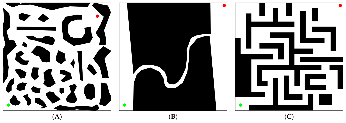
Figure 1. Example path computed for a workspace W with several obstacles.
Mathematics 09 00357 g001
Figure 2. Workspaces used in test cases (AC), respectively.
Mathematics 09 00357 g002
Figure 3. Multimodality in the path-planning problem: (a) a path with minimum length and a minimum number of control points and (b) the same path using more control points.
Mathematics 09 00357 g003
Figure 4. Exploration in the path-planning problem: (a) a path with minimum length using two control points and (b) a longer path using a single control point.
Mathematics 09 00357 g004
Figure 5. Best paths achieved by VLV-DE for test cases (AC), respectively.
Mathematics 09 00357 g005
Figure 6. Paths achieved by A* when w = 1 for test cases (AC), respectively.
Mathematics 09 00357 g006
Figure 7. Paths achieved by RRT*-Smart for test cases (AC), respectively.
Mathematics 09 00357 g007
Table 1. Details of the workspaces used in test cases (A), (B) and (C), respectively.
Test CaseObstaclesSize (m, m) p s (m, m) p t (m, m)Complexity
(A)32(100, 100)(5, 5)(87.5, 87.5)0/1E8
(B)2(100, 100)(5, 5)(97.5, 97.5)0/1E8
(C)17(100, 100)(5, 5)(97.5, 97.5)0/1E8
Table 2. Differential Evolution for Variable-Length-Vector (VLV-DE) results for test cases (A), (B) and (C).
Test Case (A)Test Case (B)Test Case (c)
Mean s ( x ) 913.266613.9666
STD1.23171.20151.5196
C.I.[8.61788, 9.3821][12.8939, 13.6394][13.4952, 14.4380]
Mean J ( m ) 2627.05703453.44414095.0317
STD ( m ) 45.962011.472848.2714
C.I. ( m ) [2612.7988, 2641.3152][3449.8850, 3457.0032][4080.0571, 4110.0064]
Best s ( x ) 91513
Best J ( m ) 2548.86963415.77573989.3064
Worst s ( x ) 111317
Worst J ( m ) 2731.27213471.73034194.8301
Table 3. A* results for test cases (A), (B) and (C).
Test Case s ( x ) J (m)
(A)1663314.1421
(B)2194374.1421
(C)2324634.1421
Table 4. RRT*-Smart results for test cases (A), (B) and (C).
Test Case s ( x ) J (m)
(A)83334.5370
(B)123562.2011
(C)154559.8692
Publisher’s Note: MDPI stays neutral with regard to jurisdictional claims in published maps and institutional affiliations.

