A Piecewise Polynomial Harmonic Nonlinear Interpolatory Reconstruction Operator on Non Uniform Grids—Adaptation around Jump Discontinuities and Elimination of Gibbs Phenomenon

Abstract

In this paper, we analyze the behavior of a nonlinear reconstruction operator called PPH around discontinuities. The acronym PPH stands for Piecewise Polynomial Harmonic, since it uses piecewise polynomials defined by means of an adaption based on the use of the weighted Harmonic mean. This study is carried out in the general case of nonuniform grids, although for some results we restrict to $\sigma$ quasi-uniform grids. In particular we analyze the numerical order of approximation close to jump discontinuities and the elimination of the Gibbs effects. We show, both theoretically and with numerical examples, that the numerical order is reduced but not completely lost as it is the case in their linear counterparts. Moreover we observe that the reconstruction is free of any Gibbs effects for sufficiently small grid sizes.

1. Introduction

Due to the extended use of reconstruction operators in many fields of application, ranging from hyperbolic conservation laws to computer aided geometric design, it is of great importance to dispose of efficient methods to build them for different situations. In general, and for the sake of simplicity, the considered functions are polynomials. High degree polynomials are, however, usually avoided because they are known to generate oscillations and undesirable effects.

Linear operators behave improperly in presence of jump discontinuities, so that different nonlinear operators have emerged to deal with this problematic. Recent approaches to deal with similar problems of functions affected by discontinuities can be found for example in [1,2,3,4,5]. And these nonlinear methods also give rise to interesting applications. To mention some of them one can refer to [6,7,8,9,10,11].

In this article we pay attention to one of these operators that was defined in [12] under the name PPH (Piecewise Polynomial Harmonic). This operator can be seen as a nonlinear counterpart of the classical four points piecewise Lagrange interpolation. The theoretical analysis as much as the practical applications were developed in uniform grids in previous articles (see, for example, [12,13,14,15,16,17,18]). In turn these reconstruction operators are the heart of the definition of associated subdivision and multiresolution schemes [5,19,20,21].

In this paper, we extend the definition of the PPH reconstruction operator to data over non uniform grids and we study some properties of this operator. In particular, we analyze the behavior of the operator in presence of jump discontinuities. We prove adaption to the jump discontinuity in the sense that some order of approximation is maintained in the area close to the discontinuity, on the contrary to what happens with linear operators that lose completely the approximation order. We also prove, as much theoretically as in numerical experiments, the absence of any Gibss phenomena.

The paper is organized as follows—in Section 2 we remind the nonlinear PPH reconstruction operator [22] on nonuniform grids. Section 3 is dedicated to study the adaption of the operator to the presence of jump discontinuities, making some emphasis in the order of approximation. In Section 4 we analyze the behavior of the operator with respect to the Gibbs phenomena. In Section 5 we present some numerical tests. Finally, some conclusions are given in Section 6.

2. A Nonlinear PPH Reconstruction Operator on Non Uniform Grids

In this section we recall the definition of the nonlinear PPH reconstruction operator on nonuniform grids, see [22]. We include the necessary elements for the rest of the article. In [22] the reconstruction operator is designed to deal with strictly convex functions, albeit it is also of interest in the case of working with piecewise smooth functions affected by isolated jump discontinuities. This will be our case of interest in this section and in the rest of the article.

Let us define a nonuniform grid $X={\left(x_i\right)}_{i\in \mathbb{Z}}$ in $\mathbb{R}.$ Let us also denote $h_i:=x_i-x_{i-1},$ the nonuniform spacing between abscissae. We consider underlying piecewise continuous functions $f\left(x\right)$ with at most a finite set of isolated corner or jump discontinuities, and let us call $f_i:=f\left(x_i\right)$ the ordinates corresponding to the point values of the function at the given abscissae. We also introduce the following notations. In first place, the second order divided differences

$$\begin{array}{cc}\hfill D_j& :=f[x_{j-1},x_j,x_{j+1}]=\frac{f_{j-1}}{h_j(h_j+h_{j+1})}-\frac{f_j}{h_j{h}_{j+1}}+\frac{f_{j+1}}{h_{j+1}(h_j+h_{j+1})},\hfill \\ \hfill D_{j+1}& :=f[x_j,x_{j+1},x_{j+2}]=\frac{f_j}{h_{j+1}(h_{j+1}+h_{j+2})}-\frac{f_{j+1}}{h_{j+1}{h}_{j+2}}+\frac{f_{j+2}}{h_{j+2}(h_{j+1}+h_{j+2})},\hfill \end{array}$$

(1)

in second place a weighted arithmetic mean of $D_j$ and $D_{j+1}$ defined as

$$M_j=w_{j,0}{D}_j+w_{j,1}{D}_{j+1},$$

(2)

with the weights

$$\begin{array}{cc}\hfill w_{j,0}& ={\displaystyle \frac{h_{j+1}+2h_{j+2}}{2(h_j+h_{j+1}+h_{j+2})}},\hfill \\ \hfill w_{j,1}& ={\displaystyle \frac{h_{j+1}+2h_j}{2(h_j+h_{j+1}+h_{j+2})}}=1-w_{j,0}.\hfill \end{array}$$

(3)

Given these ingredients in [22] we can find the following definitions, and results that we will use later.

Lemma 1.

Let us consider the set of ordinates $\{f_{j-1},f_j,f_{j+1},f_{j+2}\}$ for some $j\in \mathbb{Z}$ at the abscissae $\{x_{j-1},x_j,x_{j+1},x_{j+2}\}$ of a nonuniform grid $X={\left(x_i\right)}_{i\in \mathbb{Z}}$. Then the values $f_{j-1}$ and $f_{j+2}$ at the extremes can be expressed as

$$\begin{array}{cc}\hfill f_{j-1}& =\frac{-1}{{\gamma }_{j,-1}}({\gamma }_{j,0}{f}_j+{\gamma }_{j,1}{f}_{j+1}+{\gamma }_{j,2}{f}_{j+2})+\frac{M_j}{{\gamma }_{j,-1}},\hfill \end{array}$$

(4a)

$$\begin{array}{cc}\hfill f_{j+2}& =\frac{-1}{{\gamma }_{j,2}}({\gamma }_{j,-1}{f}_{j-1}+{\gamma }_{j,0}{f}_j+{\gamma }_{j,1}{f}_{j+1})+\frac{M_j}{{\gamma }_{j,2}},\hfill \end{array}$$

(4b)

with the constants ${\gamma }_{j,i},i=-1,0,1,2$ given by

$$\begin{array}{c}{\gamma }_{j,-1}={\displaystyle \frac{h_{j+1}+2h_{j+2}}{2h_j(h_{j+1}+h_j)(h_j+h_{j+1}+h_{j+2})}},\hfill \\ {\gamma }_{j,0}={\displaystyle \frac{1}{2h_{j+1}(h_j+h_{j+1}+h_{j+2})}}\left({\displaystyle \frac{h_{j+1}+2h_j}{h_{j+1}+h_{j+2}}}-{\displaystyle \frac{h_{j+1}+2h_{j+2}}{h_j}}\right),\hfill \\ {\gamma }_{j,1}={\displaystyle \frac{1}{2h_{j+1}(h_j+h_{j+1}+h_{j+2})}}\left({\displaystyle \frac{h_{j+1}+2h_{j+2}}{h_{j+1}+h_j}}-{\displaystyle \frac{h_{j+1}+2h_j}{h_{j+2}}}\right),\hfill \\ {\gamma }_{j,2}={\displaystyle \frac{h_{j+1}+2h_j}{2h_{j+2}(h_{j+1}+h_{j+2})(h_j+h_{j+1}+h_{j+2})}}.\hfill \end{array}$$

(5)

Definition 1.

Given $x,y\in \mathbb{R},$ and $w_x,w_y\in \mathbb{R}$ such that $w_x>0,$$w_y>0,$ and $w_x+w_y=1,$ we denote as $\tilde{V}$ the function

$$\tilde{V}(x,y)=\left\{\begin{array}{cc}{\displaystyle \frac{xy}{w_{x}y+w_{y}x}}& ifxy>0,\hfill \\ 0& otherwise.\hfill \end{array}\right.$$

(6)

Lemma 2.

If $x\ge 0$ and $y\ge 0,$ the harmonic mean is bounded as follows

$$\tilde{V}(x,y)<min\left\{{\displaystyle \frac{1}{w_x}}x,{\displaystyle \frac{1}{w_y}}y\right\}\le {\displaystyle \frac{1}{w_x}}x.$$

(7)

Next definition, which is commonly used in numerical analysis, is going to be essential through the rest of the article.

Definition 2.

An expression $e\left(h\right)=O\left(h^r\right),$$r\in \mathbb{Z}$ means that there exist $h_0>0$ and $M>0$ such that $\forall 0<h\le h_0$

$$\frac{\left|e\right(h\left)\right|}{h^r}\le M.$$

Lemma 3.

Let $a>0$ a fixed positive real number, and let $x\ge a$ and $y\ge a.$ If $|x-y|=O\left(h\right)$, and $xy>0,$ then the weighted harmonic mean is also close to the weighted arithmetic mean $M(x,y)=w_{x}x+w_{y}y,$

$$|M(x,y)-\tilde{V}(x,y)|={\displaystyle \frac{w_x{w}_y}{w_{x}y+w_{y}x}}{(x-y)}^2=O\left(h^2\right).$$

(8)

Definition 3

(PPH reconstruction). Let $X={\left(x_i\right)}_{i\in \mathbb{Z}}$ be a nonuniform mesh. Let $f={\left(f_i\right)}_{i\in \mathbb{Z}}$ a sequence in $l_{\infty }\left(\mathbb{Z}\right).$ Let $D_j$ and $D_{j+1}$ be the second order divided differences, and for each $j\in \mathbb{Z}$ let us consider the modified values $\{{\tilde{f}}_{j-1},{\tilde{f}}_j,{\tilde{f}}_{j+1},{\tilde{f}}_{j+2}\}$ built according to the following rule

• Case 1: If$|D_j|\le |D_{j+1}|$

  $$\left\{\begin{array}{cc}{\tilde{f}}_i=\hfill & f_i,j-1\le i\le j+1,\hfill \\ {\tilde{f}}_{j+2}=\hfill & \frac{-1}{{\gamma }_{j,2}}({\gamma }_{j,-1}{f}_{j-1}+{\gamma }_{j,0}{f}_j+{\gamma }_{j,1}{f}_{j+1})+\frac{{\tilde{V}}_j}{{\gamma }_{j,2}},\hfill \end{array}\right.$$

  (9)
• Case 2: If $|D_j|>|D_{j+1}|$

  $$\left\{\begin{array}{cc}{\tilde{f}}_{j-1}=\hfill & \frac{-1}{{\gamma }_{j,-1}}({\gamma }_{j,0}{f}_j+{\gamma }_{j,1}{f}_{j+1}+{\gamma }_{j,2}{f}_{j+2})+\frac{{\tilde{V}}_j}{{\gamma }_{j,-1}},\hfill \\ {\tilde{f}}_i=\hfill & f_i,j\le i\le j+2,\hfill \end{array}\right.$$

  (10)

  where ${\gamma }_{j,i},i=-1,0,1,2$ are given in (5) and ${\tilde{V}}_j=\tilde{V}(D_j,D_{j+1}),$ with $\tilde{V}$ the weighted harmonic mean defined in (6) with the weights $w_{j,0}$ and $w_{j,1}$ in (3). We define the PPH nonlinear reconstruction operator as

  $$PPH\left(x\right)=PP{H}_j\left(x\right),x\in [x_j,x_{j+1}],$$

  (11)

  where $PP{H}_j\left(x\right)$ is the unique interpolation polynomial which satisfies

  $$PP{H}_j\left(x_i\right)={\tilde{f}}_i,j-1\le i\le j+2.$$

  (12)

According to Definition 3, it is possible to establish a parallelism with Lagrange interpolation, in fact we can write the PPH reconstruction as

$$PP{H}_j\left(x\right)={\tilde{a}}_{j,0}+{\tilde{a}}_{j,1}\left(x-x_{j+\frac{1}{2}}\right)+{\tilde{a}}_{j,2}{\left(x-x_{j+\frac{1}{2}}\right)}^2+{\tilde{a}}_{j,3}{\left(x-x_{j+\frac{1}{2}}\right)}^3,$$

(13)

where the the coefficients ${\tilde{a}}_{j,i},i=0,1,2,3$ are calculated by imposing conditions (12). We explain each one of the two possible local cases, Case 1 or Case 2. The coefficients will have symmetrical expressions.

Case 1. $|D_j|\le |D_{j+1}|$, which means that a potential singularity may lay in $[x_{j+1},x_{j+2}]$. It has been proposed to replace $f_{j+2}$ with ${\tilde{f}}_{j+2}$ in Equation (9) by changing the weighted arithmetic mean in Equation (4b) for its corresponding weighted harmonic mean. This replacement has been performed to carry out a witty modification of the value ${\tilde{f}}_{j+2}$ in such a way that its difference with respect to the original $f_{j+2}$ is large in presence of a discontinuity, but remains sufficiently small in smooth areas maintaining the approximation order. Lemma 2 is crucial for the adaption in case of dealing with the presence of a jump discontinuity, while Lemma 3 plays a fundamental part in proving fourth approximation order for smooth areas of an underlying function.

In this case the coefficients ${\tilde{a}}_{j,i},i=0,1,2,3$ of the PPH polynomial read

$$\begin{array}{c}{\tilde{a}}_{j,0}={\displaystyle \frac{f_j+f_{j+1}}{2}}-{\displaystyle \frac{h_{j+1}^2}{4}}{\tilde{V}}_j,\hfill \\ {\tilde{a}}_{j,1}={\displaystyle \frac{-f_j+f_{j+1}}{h_{j+1}}}+{\displaystyle \frac{h_{j+1}^2}{4h_j+2h_{j+1}}}(D_j-{\tilde{V}}_j),\hfill \\ {\tilde{a}}_{j,2}={\tilde{V}}_j,\hfill \\ {\tilde{a}}_{j,3}=-{\displaystyle \frac{2}{2h_j+h_{j+1}}}(D_j-{\tilde{V}}_j).\hfill \end{array}$$

(14)

For our purposes, in the next sections we need to examine deeper the relation with Lagrange interpolation. In particular we get that

$$|{\tilde{f}}_{j+2}-f_{j+2}|=\frac{2h_{j+2}(h_{j+1}+h_{j+2})(h_j+h_{j+1}+h_{j+2})}{2h_j+h_{j+1}}|M_j-{\tilde{V}}_j|,$$

(15)

and considering the Lagrange interpolation polynomial written in the same form as in (13), that is

$$p_{L_j}=a_{j,0}+a_{j,1}\left(x-x_{j+\frac{1}{2}}\right)+a_{j,2}{\left(x-x_{j+\frac{1}{2}}\right)}^2+a_{j,3}{\left(x-x_{j+\frac{1}{2}}\right)}^3,$$

(16)

we get that the difference of these coefficients with the ones of $PP{H}_j\left(x\right)$ is given by

$$\begin{array}{c}{\tilde{a}}_{j,0}-a_{j,0}={\displaystyle \frac{h_{j+1}^2}{4}}\left(M_j-{\tilde{V}}_j\right),\hfill \\ {\tilde{a}}_{j,1}-a_{j,1}={\displaystyle \frac{h_{j+1}^2}{4h_j+2h_{j+1}}}(M_j-{\tilde{V}}_j),\hfill \\ {\tilde{a}}_{j,2}-a_{j,2}=-(M_j-{\tilde{V}}_j),\hfill \\ {\tilde{a}}_{j,3}-a_{j,3}=-{\displaystyle \frac{2}{2h_j+h_{j+1}}}(M_j-{\tilde{V}}_j).\hfill \end{array}$$

(17)

Case 2. $|D_j|>|D_{j+1}|$, which means that a possible singularity lies in $[x_{j-1},x_j]$. In this case, in Definition 3, the value $f_{j-1}$ is replaced with ${\tilde{f}}_{j-1}$ by using expression (10). Similar comments apply in this case due to symmetry considerations. The coefficients for the polynomial (13) now read

$$\begin{array}{c}{\tilde{a}}_{j,0}={\displaystyle \frac{f_j+f_{j+1}}{2}}-{\displaystyle \frac{h_{j+1}^2}{4}}{\tilde{V}}_j,\hfill \\ {\tilde{a}}_{j,1}={\displaystyle \frac{-f_j+f_{j+1}}{h_{j+1}}}+{\displaystyle \frac{h_{j+1}^2}{2h_{j+1}+4h_{j+2}}}(-D_{j+1}+{\tilde{V}}_j),\hfill \\ {\tilde{a}}_{j,2}={\tilde{V}}_j,\hfill \\ {\tilde{a}}_{j,3}=-{\displaystyle \frac{2}{h_{j+1}+2h_{j+2}}}(-D_{j+1}+{\tilde{V}}_j).\hfill \end{array}$$

(18)

The expressions relating the coefficients of the PPH polynomial with the Lagrange interpolation polynomial now write

$$|{\tilde{f}}_{j-1}-f_{j-1}|=\frac{2h_j(h_{j+1}+h_j)(h_j+h_{j+1}+h_{j+2})}{2h_{j+2}+h_{j+1}}|M_j-{\tilde{V}}_j|.$$

(19)

$$\begin{array}{c}{\tilde{a}}_{j,0}-a_{j,0}={\displaystyle \frac{h_{j+1}^2}{4}}\left(M_j-{\tilde{V}}_j\right),\hfill \\ {\tilde{a}}_{j,1}-a_{j,1}=-{\displaystyle \frac{h_{j+1}^2}{2h_{j+1}+4h_{j+2}}}(M_j-{\tilde{V}}_j),\hfill \\ {\tilde{a}}_{j,2}-a_{j,2}=-(M_j-{\tilde{V}}_j),\hfill \\ {\tilde{a}}_{j,3}-a_{j,3}={\displaystyle \frac{2}{2h_{j+2}+h_{j+1}}}(M_j-{\tilde{V}}_j).\hfill \end{array}$$

(20)

In next section, we will study the approximation order of the PPH reconstruction operator in presence of isolated jump discontinuities.

3. Approximation Order around Jump Discontinuities

We are going to study the approximation order of the given reconstruction for functions of class $C^4\left(\mathbb{R}\right)$ with an isolated jump discontinuity at a given point $\mu .$ We consider only the case of working with $\sigma$ quasi-uniform grids, according with the following definition.

Definition 4.

A nonuniform mesh $X={\left(x_i\right)}_{i\in \mathbb{Z}}$ is said to be a σ quasi-uniform mesh if there exist $h_{min}=\underset{i\in \mathbb{Z}}{min}{h}_i,$ $h_{max}=\underset{i\in \mathbb{Z}}{max}{h}_i,$ and a finite constant σ such that $\frac{h_{max}}{h_{min}}\le \sigma .$

In what follows we give a proposition proving full order accuracy for convex regions of the function, that is fourth order accuracy, and observing that the approximation order is reduced to second order close to the singularities and to third order close to inflection points. We would like to focuss especial attention to the intervals around the discontinuity where the order is reduced, but not completely lost.

Theorem 1.

Let $f\left(x\right)$ be a function of class $C^4(\mathbb{R}\setminus \left\{\mu \right\}),$ with a jump discontinuity at the point $\mu .$ Let $X={\left(x_i\right)}_{i\in \mathbb{Z}}$ be a σ quasi-uniform mesh in $\mathbb{R},$ with $h_i=x_i-x_{i-1},\forall i\in \mathbb{Z},$ and $f={\left(f_i\right)}_{i\in \mathbb{Z}},$ the sequence of point values of the function $f\left(x\right),$$f_i=f\left(x_i\right).$ Let us consider $j\in \mathbb{Z}$ such that $\mu \in [x_j,x_{j+1}],$$a>0,$ a fixed positive real number, Ω the set of all inflexion points of $f\left(x\right),$ and $d(x,\Omega )$ the distance function defined by

$$d(x,\Omega ):=\left\{\begin{array}{cc}min\left\{\right|x-\omega |:\omega \in \Omega \}\hfill & \Omega \ne \varnothing ,\hfill \\ +\infty \hfill & \Omega =\varnothing .\hfill \end{array}\right.$$

Then, the reconstruction $PPH\left(x\right)$ satisfies

1. 

In $x\in [x_i,x_{i+1}],$$i\ne j-1,j,j+1,$ if $D_i{D}_{i+1}>0,$ and $d(x_{i-1},\Omega )\ge a,$$d(x_{i+2},\Omega )\ge a$ then

$$\underset{x\in [x_i,x_{i+1}]}{max}|f\left(x\right)-PPH\left(x\right)|=O\left(h^4\right),$$

2. 

In $x\in [x_i,x_{i+1}],$$i\ne j-1,j,j+1,$ if $D_i{D}_{i+1}>0,$ and $d(x_{i-1},\Omega )<a,$ or $d(x_{i+2},\Omega )<a$ then

$$\underset{x\in [x_i,x_{i+1}]}{max}|f\left(x\right)-PPH\left(x\right)|=O\left(h^{4-p}\right),with0\le p<1.$$

3. 

In $x\in [x_i,x_{i+1}],$$i\ne j-1,j,j+1,$ if $D_i{D}_{i+1}\le 0,$

$$\underset{x\in [x_i,x_{i+1}]}{max}|f\left(x\right)-PPH\left(x\right)|=O\left(h^3\right),$$

4. 

In $x\in [x_{j-1},x_j]\cup [x_{j+1},x_{j+2}],$

$$\underset{x\in [x_{j-1},x_j]\cup [x_{j+1},x_{j+2}]}{max}|f\left(x\right)-PPH\left(x\right)|=O\left(h^2\right),$$

where $h=\underset{i\in \mathbb{Z}}{max}\left\{h_i\right\}.$

Proof. 

We do the proof point by point.

1. 

Given $x\in [x_i,x_{i+1}],$ the reconstruction operator is built as $PPH\left(x\right)=PP{H}_i\left(x\right).$

From Equations (2) and (6) we can write

$$M_i-{\tilde{V}}_i=\left\{\begin{array}{cc}{\displaystyle \frac{w_{i,0}{w}_{i,1}{(D_{i+1}-D_i)}^2}{w_{i,0}{D}_{i+1}+w_{i,1}{D}_i}}& \mathrm{if}{D}_i{D}_{i+1}>0,\hfill \\ M_i& \mathrm{otherwise}.\hfill \end{array}\right.$$

(21)

From hypothesis we have that the initial data are strictly convex in the considered area $[x_{i-1},x_{i+2}]$ (for a concave function the arguments remain the same) and therefore they satisfy $f^{″}\left(x\right)\ge b>0,\forall x\in [x_{i-1},x_{i+2}],$ for some $b>0.$ Since second order divided differences amount to second derivatives at an intermediate point divided by two, i.e.,

$$D_i=\frac{f^{″}\left({\mu }_1\right)}{2!},D_{i+1}=\frac{f^{″}\left({\mu }_2\right)}{2!},$$

with ${\mu }_1\in (x_{i-1},x_{i+1})$ and ${\mu }_2\in (x_i,x_{i+2}).$ Therefore, we have

$$D_i=O\left(1\right),D_{i+1}=O\left(1\right)\mathrm{and}{D}_{i+1}-D_i=O\left(h\right),$$

and from (21) we get that

$$\begin{array}{cc}\hfill |M_i-{\tilde{V}}_i|& =O\left(h^2\right).\hfill \end{array}$$

(22)

Plugging this information into (17) if $|D_i|\le |D_{i+1}|,$ or into (20) if $|D_i|>|D_{i+1}|,$ we get that

$$\begin{array}{cc}\hfill |{\tilde{a}}_{i,s}-a_{i,s}|& =O\left(h^{4-s}\right),s=0,1,2,3.\hfill \end{array}$$

(23)

Thus

$$|PP{H}_i\left(x\right)-p_{L_i}\left(x\right)|\le \sum _{s=0}^3|{\tilde{a}}_{i,s}-a_{i,s}|\left|{\left(x-x_{i+\frac{1}{2}}\right)}^s\right|=O\left(h^4\right),$$

where $p_{L_i}\left(x\right)$ is the Lagrange interpolatory polynomial. Taking into account again the triangular inequality

$$|f\left(x\right)-PP{H}_i\left(x\right)|\le |f\left(x\right)-p_{L_i}\left(x\right)|+|p_{L_i}\left(x\right)-PP{H}_i\left(x\right)|=O\left(h^4\right),$$

using that Lagrange interpolation also attains fourth order accuracy.

2. 

We now prove Point 2. Since $d(x_{i-1},\Omega )<a,$ or $d(x_{i+2},\Omega )<a,$ and depending on the exact distance to the inflection point we encounter $D_i=O\left(h^p\right),$$D_{i+1}=O\left(h^p\right),$ with $0\le p<1.$ Then from Equation (21) we directly get $|M_i-{\tilde{V}}_i|=O\left(h^{2-p}\right),$ and the rest of the proof follows exactly the same track as in Point 1, giving the enunciated result.

3. 

For proving Point 3, we observe that in this case $|M_i-{\tilde{V}}_i|=|M_i|=O\left(h\right),$ and again following the same track as in previous points we get

$$\begin{array}{cc}\hfill |{\tilde{a}}_{i,s}-a_{i,s}|& =O\left(h^{3-s}\right),s=0,1,2,3,\hfill \\ \hfill |PP{H}_i\left(x\right)-p_{L_i}\left(x\right)|& \le \sum _{s=0}^3|{\tilde{a}}_{i,s}-a_{i,s}|\left|{\left(x-x_{i+\frac{1}{2}}\right)}^s\right|=O\left(h^3\right),\hfill \\ \hfill |f\left(x\right)-PP{H}_i\left(x\right)|& \le |f\left(x\right)-p_{L_i}\left(x\right)|+|p_{L_i}\left(x\right)-PP{H}_i\left(x\right)|=O\left(h^3\right),\hfill \end{array}$$

and therefore in this case the accuracy is reduced to third order.

4. 

In order to prove Point 4, let us suppose without lost of generalization that $x\in [x_{j-1},x_j].$ The other case it is proven analogously. Since by hypothesis the function $f\left(x\right)$ is smooth in $[x_{j-2},x_j]$, and it presents a jump discontinuity at the interval $[x_j,x_{j+1}]$ we have $D_{j-1}=O\left(1\right)$ and $D_j=O(1/h^2).$ Therefore $|D_{j-1}|\le |D_j|$.

Let $p_{L{2}_{j-1}}\left(x\right)$ be the second degree Lagrange interpolatory polynomial built using the three pairs of values $(x_{j-2},f_{j-2}),(x_{j-1},f_{j-1}),(x_j,f_j)$.

$$\begin{array}{c}\hfill p_{L{2}_{j-1}}\left(x\right)={\widehat{a}}_{j-1,0}+{\widehat{a}}_{j-1,1}\left(x-x_{j-\frac{1}{2}}\right)+{\widehat{a}}_{j-1,2}{\left(x-x_{j-\frac{1}{2}}\right)}^2,\end{array}$$

where

$$\begin{array}{c}{\widehat{a}}_{j-1,0}={\displaystyle \frac{f_{j-1}+f_j}{2}}-{\displaystyle \frac{h_j^2}{4}}{D}_{j-1},\hfill \\ {\widehat{a}}_{j-1,1}={\displaystyle \frac{-f_{j-1}+f_j}{h_j}},\hfill \\ {\widehat{a}}_{j-1,2}=D_{j-1}.\hfill \end{array}$$

(24)

The difference between these coefficients and the ones of $PP{H}_{j-1}\left(x\right)$ shown in Equation (14) is given by

$$\begin{array}{c}{\tilde{a}}_{j-1,0}-{\widehat{a}}_{j-1,0}={\displaystyle \frac{h_j^2}{4}}\left(D_{j-1}-{\tilde{V}}_{j-1}\right),\hfill \\ {\tilde{a}}_{j-1,1}-{\widehat{a}}_{j-1,1}={\displaystyle \frac{h_j^2}{4h_{j-1}+2h_j}}(D_{j-1}-{\tilde{V}}_{j-1}),\hfill \\ {\tilde{a}}_{j-1,2}-{\widehat{a}}_{j-1,2}=-(D_{j-1}-{\tilde{V}}_{j-1}),\hfill \\ {\tilde{a}}_{j-1,3}=-{\displaystyle \frac{2}{2h_{j-1}+h_j}}(D_{j-1}-{\tilde{V}}_{j-1}).\hfill \end{array}$$

(25)

At this stage we distinguish two cases:

4.1. 

$D_{j-1}{D}_j>0$.

Taking into account Equations (6), (7) and (25) and the triangular inequality we obtain

$$\begin{array}{cc}\hfill & |\tilde{V}(D_{j-1},D_j)|\le {\displaystyle \frac{1}{w_{j-1,0}}}\left|D_{j-1}\right|,\hfill \\ \hfill & |D_{j-1}-{\tilde{V}}_{j-1}|\le |D_{j-1}|+{\displaystyle \frac{1}{w_{j-1,0}}}|D_{j-1}|={\displaystyle \frac{1+w_{j-1,0}}{w_{j-1,0}}}\left|D_{j-1}\right|=O\left(1\right),\hfill \\ \hfill & |{\tilde{a}}_{j-1,s}-{\widehat{a}}_{j-1,s}|=O\left(h^{2-s}\right),s=0,1,2,3,\hfill \\ \hfill & |PP{H}_{j-1}\left(x\right)-p_{L{2}_{j-1}}\left(x\right)|\le \sum _{s=0}^3|{\tilde{a}}_{j-1,s}-{\widehat{a}}_{j-1,s}|\left|{\left(x-x_{j-\frac{1}{2}}\right)}^s\right|=O\left(h^2\right),\hfill \\ \hfill & |f\left(x\right)-PP{H}_{j-1}\left(x\right)|\le |f\left(x\right)-p_{L{2}_{j-1}}\left(x\right)|+|p_{L{2}_{j-1}}\left(x\right)-PP{H}_{j-1}\left(x\right)|=O\left(h^2\right).\hfill \end{array}$$

4.2. 

$D_{j-1}{D}_j\le 0$.

Equations (6) and (25) and the triangular inequality lead us to

$$\begin{array}{cc}\hfill & {\tilde{V}}_{j-1}=0,\hfill \\ \hfill & |D_{j-1}-{\tilde{V}}_{j-1}|=O\left(1\right),\hfill \\ \hfill & |{\tilde{a}}_{j-1,s}-{\widehat{a}}_{j-1,s}|=O\left(h^{2-s}\right),s=0,1,2,3,\hfill \\ \hfill & |PP{H}_{j-1}\left(x\right)-p_{L{2}_{j-1}}\left(x\right)|\le \sum _{s=0}^3|{\tilde{a}}_{j-1,s}-{\widehat{a}}_{j-1,s}|\left|{\left(x-x_{j-\frac{1}{2}}\right)}^s\right|=O\left(h^2\right),\hfill \\ \hfill & |f\left(x\right)-PP{H}_{j-1}\left(x\right)|\le |f\left(x\right)-p_{L{2}_{j-1}}\left(x\right)|+|p_{L{2}_{j-1}}\left(x\right)-PP{H}_{j-1}\left(x\right)|=O\left(h^2\right).\hfill \end{array}$$

And these last chains of equations finish the proof.

□

We observe that close to the jump discontinuity, that is, in the intervals $[x_{j-1},x_j]$ and $[x_{j+1},x_{j+2}],$ we do not lose all accuracy, but we maintain at least second order accuracy. Unfortunately, in the central interval $[x_j,x_{j+1}]$ containing the singularity this approach does not allow us to obtain any gain with respect to other reconstruction operators.

Remark 1.

Notice that linear reconstruction operators based on an stencil of four points typically lose the approximation order in three intervals around discontinuities, while the introduced nonlinear reconstruction operator only loses completely the aproximation order in the interval containing the jump discontinuity and maintains at least second order accuracy, that is, $O\left(h^2\right),$ in the adjacent intervals. In the interval containing the jump discontinuity the approximation order is lost also in the nonlinear reconstruction strategy, since with point values of the function it is impossible to detect the exact position of the jump discontinuity.

Remark 2.

The order reduction due to inflection points can be tackled using a translation strategy in the definition of the Harmonic mean, to avoid arguments of different signs. This strategy complicates the definition of the operator, but it has been satisfactorily introduced on various occasions [12,23]. In practice the translation is needed not only at the interval containing the inflection point, but also in adjacent intervals.

4. Analysis of Gibbs Phenomena around Jump Discontinuities

In this section we are going to give a result analyzing the behavior of the proposed nonlinear reconstruction with respect to the generation of possible Gibbs effects due to the presence of jump discontinuities in the underlying function. In particular we prove the following proposition.

Before enunciating the theorem we introduce some definitions.

Definition 5.

Given $X^0={\left\{x_i\right\}}_{i\in \mathbb{Z}}$ a σ quasi-uniform grid in $\mathbb{R},$ we define, for $k\in \mathbb{N}$ (the larger the k the larger the resolution), the set of nested grids given by $X^k={\left\{x_i^k\right\}}_{i\in \mathbb{Z}},$ where $x_{2i}^k=x_i^{k-1}$ and $x_{2i+1}^k=\frac{x_i^{k-1}+x_{i+1}^{k-1}}{2}.$

Let us also denote $\left[f\right]$ the size of a jump discontinuity, $r_j^k\left(x\right)$ the straight line joining the points $(x_j^k,f_j^k)$ and $(x_{j+1}^k,f_{j+1}^k),$$d_i^k\left(x\right),i=j-1,j,j+1$ the vertical distance from the reconstruction $PP{H}_j^k\left(x\right)$ to the horizontal line passing through the middle point of $(x_j^k,f_j^k)$ and $(x_{j+1}^k,f_{j+1}^k).$ The respective expressions come given by

$\left[f\right]=f_{j+1}^k-f_j^k,$

$r_j^k\left(x\right)={\displaystyle \frac{f_j^k+f_{j+1}^k}{2}}+{\displaystyle \frac{f_{j+1}^k-f_j^k}{h_{j+1}^k}}(x-x_{j+\frac{1}{2}}^k),$

$d_i^k\left(x\right)=PP{H}_i^k\left(x\right)-{\displaystyle \frac{f_i^k+f_{i+1}^k}{2}}.$

We will also use $r_{max}^k$ as the maximum distance between $PP{H}_j^k\left(x\right)$ and $r_j^k\left(x\right)$ measured perpendicularly to $r_j^k\left(x\right).$

Theorem 2.

Let $X^k={\left\{x_i^k\right\}}_{i\in \mathbb{Z}},k\in \mathbb{N}\cup \left\{0\right\}$ be a set of nested σ quasi-uniform grids in $\mathbb{R}.$ Let $f\in C^4\left(\mathbb{R}\right)$ be a function with four continuous derivatives in all the real line with an isolated jump discontinuity at the abscissa μ located at a certain $[x_j^k,x_{j+1}^k]$ for each $k,$ where j depends on $k.$ Then, $\exists k_0:\forall k\ge k_0$ the reconstruction $PP{H}^k\left(x\right)$ associated to the data $f^k:={\left(f\left(x_i^k\right)\right)}_{i\in \mathbb{Z}}$ does not generate Gibbs phenomena. In particular, the following statements hold:

1. 

$\left|\right|PP{H}^k\left(x\right)-f\left(x\right){\left|\right|}_{L^{\infty }}=O\left({\left(h^k\right)}^4\right)in(-\infty ,x_{j-1}^k]\cup [x_{j+2}^k,\infty ),$

2. 

$\left|d_{j-1}^k\left(x\right)\right|=O\left(h^k\right),$

3. 

$\left|d_{j+1}^k\left(x\right)\right|=O\left(h^k\right),$

4. 

$PP{H}_j^k\left(x\right)$ lies inside the rectangle $[x_j^k,x_{j+1}^k]\times [f_j^k,f_{j+1}^k],$

5. 

$r_{max}^k=O\left(h^k\right),$

where $h^k:=\underset{i\in \mathbb{Z}}{max}\left\{h_i^k\right\}.$

Proof. 

Let us consider $k$ large enough, $k\ge k_0,$ such that

$$\begin{array}{cc}\hfill & \left|{\displaystyle \frac{\left[f\right]}{h_{j+1}^k}}\right|>\left|{\displaystyle \frac{f_j^k-f_{j-1}^k}{h_j^k}}\right|,\hfill \end{array}$$

(26)

$$\begin{array}{cc}\hfill & \left|{\displaystyle \frac{\left[f\right]}{h_{j+1}^k}}\right|>\left|{\displaystyle \frac{f_{j+2}^k-f_{j+1}^k}{h_{j+2}^k}}\right|.\hfill \end{array}$$

(27)

Then

$$\begin{array}{cc}\hfill & D_{j-1}^k=O\left(1\right),\hfill \\ \hfill & D_j^k={\displaystyle \frac{{\displaystyle \frac{f_{j+1}^k-f_j^k}{h_{j+1}^k}}-{\displaystyle \frac{f_j^k-f_{j-1}^k}{h_j^k}}}{h_j^k+h_{j+1}^k}}=O\left({\displaystyle \frac{\left[f\right]}{{\left(h^k\right)}^2}}\right),\hfill \end{array}$$

(28)

$$\begin{array}{cc}\hfill & D_{j+1}^k={\displaystyle \frac{{\displaystyle \frac{f_{j+2}^k-f_{j+1}^k}{h_{j+2}^k}}-{\displaystyle \frac{f_{j+1}^k-f_j^k}{h_{j+1}^k}}}{h_{j+1}^k+h_{j+2}^k}}=-O\left({\displaystyle \frac{\left[f\right]}{{\left(h^k\right)}^2}}\right),\hfill \\ \hfill & D_{j+2}^k=O\left(1\right).\hfill \end{array}$$

(29)

and from (28), (29) and (6) we get

$$\begin{array}{cc}\hfill sgn\left(D_j^k\right)=sgn& \left(\left[f\right]\right)\ne sgn\left(D_{j+1}^k\right),\hfill \\ \hfill & {\tilde{V}}_j^k=0.\hfill \end{array}$$

(30)

We carry out the rest of the proof addressing point after point.

1. Since only three intervals are affected by the jump discontinuity for construction, then $\forall k$

$$\left|\right|PP{H}^k\left(x\right)-f\left(x\right){\left|\right|}_{L^{\infty }}=O\left({\left(h^k\right)}^4\right)\mathrm{in}(-\infty ,x_{j-1}^k]\cup [x_{j+2}^k,\infty ).$$

2. We are going to show now that the oscillations due to the presence of the discontinuity diminish at the interval $[x_{j-1}^k,x_j^k]$ with k increasing.

In $[x_{j-1}^k,x_j^k]$ the PPH reconstruction amounts to

$$PP{H}_{j-1}^k\left(x\right)={\tilde{a}}_{j-1,0}^k+{\tilde{a}}_{j-1,1}^k\left(x-x_{j-\frac{1}{2}}^k\right)+{\tilde{a}}_{j-1,2}^k{\left(x-x_{j-\frac{1}{2}}^k\right)}^2+{\tilde{a}}_{j-1,3}^k{\left(x-x_{j-\frac{1}{2}}^k\right)}^3.$$

(31)

As $|D_{j-1}^k|\le |D_j^k|,$ the coefficients are given by (14) adapted to the interval $j-1$

$$\begin{array}{c}{\tilde{a}}_{j-1,0}^k={\displaystyle \frac{f_{j-1}^k+f_j^k}{2}}-{\displaystyle \frac{{\left(h_j^k\right)}^2}{4}}{\tilde{V}}_{j-1}^k\hfill \\ {\tilde{a}}_{j-1,1}^k={\displaystyle \frac{-f_{j-1}^k+f_j^k}{h_j^k}}+{\displaystyle \frac{{\left(h_j^k\right)}^2}{4h_{j-1}^k+2h_j^k}}(D_{j-1}^k-{\tilde{V}}_{j-1}^k)\hfill \\ {\tilde{a}}_{j-1,2}^k={\tilde{V}}_{j-1}^k\hfill \\ {\tilde{a}}_{j-1,3}^k=-{\displaystyle \frac{2}{2h_{j-1}^k+h_j^k}}(D_{j-1}^k-{\tilde{V}}_{j-1}^k).\hfill \end{array}$$

(32)

Taking into account property (7) of the harmonic mean, we can write

$$\begin{array}{cc}\hfill |{\tilde{V}}_{j-1}^k|=|{\tilde{V}}_{j-1}^k(D_{j-1}^k,D_j^k)|& \le min\left\{{\displaystyle \frac{1}{w_{j-1,0}^k}}|D_{j-1}^k|,{\displaystyle \frac{1}{w_{j-1,1}^k}}\left|D_j^k\right|\right\}\hfill \\ \hfill & \le {\displaystyle \frac{1}{w_{j-1,0}^k}}|D_{j-1}^k|\le 2\sigma |D_{j-1}^k|.\hfill \end{array}$$

Considering (31), the distance $d_{j-1}^k\left(x\right)$ can be bounded by

$$\begin{array}{cc}\hfill \left|d_{j-1}^k\left(x\right)\right|& =\left|PP{H}_{j-1}^k\left(x\right)-{\displaystyle \frac{f_{j-1}^k+f_j^k}{2}}\right|=\left|-{\displaystyle \frac{{\left(h_j^k\right)}^2}{4}}{\tilde{V}}_{j-1}^k+{\tilde{a}}_{j-1,1}^k\left(x-x_{j-\frac{1}{2}}^k\right)\right.\hfill \\ \hfill & +\left.{\tilde{a}}_{j-1,2}^k{\left(x-x_{j-\frac{1}{2}}^k\right)}^2+{\tilde{a}}_{j-1,3}^k{\left(x-x_{j-\frac{1}{2}}^k\right)}^3\right|=O\left(h^k\right),\hfill \end{array}$$

where $h^k:=\underset{i\in \mathbb{Z}}{max}\left\{h_i^k\right\}.$

3. In $[x_{j+1}^k,x_{j+2}^k],$ applying arguments based on symmetry and taking into account that $|D_{j+1}^k|\ge |D_{j+2}^k|$ we also get that $\left|d_{j+1}^k\left(x\right)\right|=O\left(h^k\right).$

4. In $[x_j^k,x_{j+1}^k],$ as ${\tilde{V}}_j^k=0$ due to (30), the expression of $PP{H}_j^k\left(x\right)$ according to (13), (14), (18) will be

$$PP{H}_j^k\left(x\right)={\displaystyle \frac{f_j^k+f_{j+1}^k}{2}}+{\tilde{a}}_{1,j}^k\left(x-x_{j+\frac{1}{2}}^k\right)+{\tilde{a}}_{3,j}^k{\left(x-x_{j+\frac{1}{2}}^k\right)}^3.$$

(33)

At this point we consider two subcases depending on $|D_j^k|$ and $|D_{j+1}^k|$

4.1$|D_j^k|\le |D_{j+1}^k|$

We can write

$$d_j^k\left(x\right)={\tilde{a}}_{1,j}^k\left(x-x_{j+\frac{1}{2}}^k\right)+{\tilde{a}}_{3,j}^k{\left(x-x_{j+\frac{1}{2}}^k\right)}^3=\left(x-x_{j+\frac{1}{2}}^k\right)E_j^k\left(x\right),$$

(34)

where

$$E_j^k\left(x\right)={\displaystyle \frac{f_{j+1}^k-f_j^k}{h_{j+1}^k}}+{\displaystyle \frac{D_j^k}{4h_j^k+2h_{j+1}^k}}\left({\left(h_{j+1}^k\right)}^2-4{(x-x_{j+\frac{1}{2}}^k)}^2\right).$$

The maximum value of the function $d_j^k\left(x\right)$ in the interval $[x_j^k,x_{j+1}^k]$ is either at the extremes of the interval or among any possible critical point $x_c$ verifying ${\left(d_j^k\right)}^{\prime }\left(x_c\right)=0.$ At the extremes of the interval we have $\left|d_j^k\left(x_j^k\right)\right|=\left|d_j^k\left(x_{j+1}^k\right)\right|=\frac{1}{2}\left|f_{j+1}^k-f_j^k\right|,$ and the condition is satisfied. We are going to prove that the local reconstruction $PP{H}_j^k\left(x\right)$ lies inside the rectangle $[x_j^k,x_{j+1}^k]\times [f_j^k,f_{j+1}^k]$ since any critical point $x_c$ of the function $d_j^k\left(x\right)$ falls outside the interval $[x_j^k,x_{j+1}^k].$ For this purpose, we shall prove that ${\left(PP{H}_j^k\right)}^{\prime }\left(x\right)\ne 0\forall x\in [x_j^k,x_{j+1}^k].$ We start computing ${\left(PP{H}_j^k\right)}^{\prime }\left(x\right)$ and ${\left(PP{H}_j^k\right)}^{″}\left(x\right),$

$$\begin{array}{cc}\hfill {\left(PP{H}_j^k\right)}^{\prime }\left(x\right)& ={\displaystyle \frac{f_{j+1}^k-f_j^k}{h_{j+1}^k}}+{\displaystyle \frac{D_j^k}{4h_j^k+2h_{j+1}^k}}\left({\left(h_{j+1}^k\right)}^2-12{(x-x_{j+\frac{1}{2}}^k)}^2\right),\hfill \\ \hfill {\left(PP{H}_j^k\right)}^{″}\left(x\right)& =-24{\displaystyle \frac{D_j^k}{4h_j^k+2h_{j+1}^k}}(x-x_{j+\frac{1}{2}}^k).\hfill \end{array}$$

(35)

Last equations show that ${\left(PP{H}_j^k\right)}^{\prime }\left(x\right)$ is symmetric respect to the vertical axis passing through $x=x_{j+\frac{1}{2}}^k$ where it reaches a local maximum since ${\left(PP{H}_j^k\right)}^{″}\left(x_{j+\frac{1}{2}}^k\right)=0.$

Evaluating (35) at $x_j^k,x_{j+\frac{1}{2}}^k$ and $x_{j+1}^k$ we obtain

$$\begin{array}{cc}\hfill {\left(PP{H}_j^k\right)}^{\prime }\left(x_j\right)& ={\left(PP{H}_j^k\right)}^{\prime }\left(x_{j+1}\right)={\displaystyle \frac{f_{j+1}^k-f_j^k}{h_{j+1}^k}}-{\displaystyle \frac{D_j^k{\left(h_{j+1}^k\right)}^2}{4(2h_j^k+h_{j+1}^k)}},\hfill \end{array}$$

(36)

$$\begin{array}{cc}\hfill {\left(PP{H}_j^k\right)}^{\prime }\left(x_{j+\frac{1}{2}}^k\right)& ={\displaystyle \frac{f_{j+1}^k-f_j^k}{h_{j+1}^k}}+{\displaystyle \frac{D_j^k{\left(h_{j+1}^k\right)}^2}{2(2h_j^k+h_{j+1}^k)}}.\hfill \end{array}$$

(37)

From (37) and (30) we get

$$sgn\left({\left(PP{H}_j^k\right)}^{\prime }\left(x_{j+\frac{1}{2}}^k\right)\right)=sgn\left(\left[f\right]\right).$$

(38)

To analyze the sign of ${\left(PP{H}_j^k\right)}^{\prime }\left(x_j\right)$ we replace in (36) $D_j^k$ by its expression (28)

$${\left(PP{H}_j^k\right)}^{\prime }\left(x_j\right)={\displaystyle \frac{f_{j+1}^k-f_j^k}{h_{j+1}^k}}-{\displaystyle \frac{1}{4}}{\displaystyle \frac{{\left(h_{j+1}^k\right)}^2}{{\left(h_{j+1}^k\right)}^2+3h_j^k{h}_{j+1}^k+2{\left(h_j^k\right)}^2}}\left[{\displaystyle \frac{f_{j+1}^k-f_j^k}{h_{j+1}^k}}-{\displaystyle \frac{f_j^k-f_{j-1}^k}{h_j^k}}\right],$$

and we consider two subcases depending on the sign of $\left[f\right],$

4.1.1$sgn\left[f\right]>0.$ From (26), ${\displaystyle \frac{\left[f\right]}{h_{j+1}^k}}>-{\displaystyle \frac{f_j^k-f_{j-1}^k}{h_j^k}},$ and we get

$$\begin{array}{cc}\hfill {\left(PP{H}_j^k\right)}^{\prime }& \left(x_j\right)>{\displaystyle \frac{f_{j+1}^k-f_j^k}{h_{j+1}^k}}-{\displaystyle \frac{1}{4}}{\displaystyle \frac{{\left(h_{j+1}^k\right)}^2}{{\left(h_{j+1}^k\right)}^2+3h_j^k{h}_{j+1}^k+2{\left(h_j^k\right)}^2}}2{\displaystyle \frac{f_{j+1}^k-f_j^k}{h_{j+1}^k}}\hfill \\ \hfill & ={\displaystyle \frac{f_{j+1}^k-f_j^k}{h_{j+1}^k}}\left[1-{\displaystyle \frac{1}{2}}{\displaystyle \frac{{\left(h_{j+1}^k\right)}^2}{{\left(h_{j+1}^k\right)}^2+3h_j^k{h}_{j+1}^k+2{\left(h_j^k\right)}^2}}\right]>{\displaystyle \frac{1}{2}}{\displaystyle \frac{f_{j+1}^k-f_j^k}{h_{j+1}^k}}>0.\hfill \end{array}$$

4.1.2$sgn\left[f\right]<0.$ Again from (26), ${\displaystyle \frac{\left[f\right]}{h_{j+1}^k}}<-{\displaystyle \frac{f_j^k-f_{j-1}^k}{h_j^k}},$ and we get

$$\begin{array}{cc}\hfill {\left(PP{H}_j^k\right)}^{\prime }& \left(x_j\right)<{\displaystyle \frac{f_{j+1}^k-f_j^k}{h_{j+1}^k}}-{\displaystyle \frac{1}{4}}{\displaystyle \frac{{\left(h_{j+1}^k\right)}^2}{{\left(h_{j+1}^k\right)}^2+3h_j^k{h}_{j+1}^k+2{\left(h_j^k\right)}^2}}2{\displaystyle \frac{f_{j+1}^k-f_j^k}{h_{j+1}^k}}\hfill \\ \hfill & ={\displaystyle \frac{f_{j+1}^k-f_j^k}{h_{j+1}^k}}\left[1-{\displaystyle \frac{1}{2}}{\displaystyle \frac{{\left(h_{j+1}^k\right)}^2}{{\left(h_{j+1}^k\right)}^2+3h_j^k{h}_{j+1}^k+2{\left(h_j^k\right)}^2}}\right]<{\displaystyle \frac{1}{2}}{\displaystyle \frac{f_{j+1}^k-f_j^k}{h_{j+1}^k}}<0.\hfill \end{array}$$

In both subcases $sgn\left({\left(PP{H}_j^k\right)}^{\prime }\left(x_j^k\right)\right)=sgn\left({\left(PP{H}_j^k\right)}^{\prime }\left(x_{j+1}^k\right)\right)=sgn\left(\left[f\right]\right),$ which together with expression (38) allow us to write $sgn\left({\left(PP{H}_j^k\right)}^{\prime }\left(x\right)\right)=sgn\left(\left[f\right]\right)\forall x\in [x_j^k,x_{j+1}^k],$ and therefore ${\left(PP{H}_j^k\right)}^{\prime }\left(x\right)\ne 0\forall x\in [x_j^k,x_{j+1}^k],$ what amounts to say that there is not local maximum value of $PP{H}_j^k\left(x\right)$ inside the interval.

4.2$|D_j^k|>|D_{j+1}^k|$

In this case

$$E_j^k\left(x\right)={\displaystyle \frac{f_{j+1}^k-f_j^k}{h_{j+1}^k}}-{\displaystyle \frac{D_{j+1}^k}{4h_{j+2}^k+2h_{j+1}^k}}\left({\left(h_{j+1}^k\right)}^2-4{(x-x_{j+\frac{1}{2}}^k)}^2\right),$$

$$\begin{array}{cc}\hfill {\left(PP{H}_j^k\right)}^{\prime }\left(x\right)& ={\displaystyle \frac{f_{j+1}^k-f_j^k}{h_{j+1}^k}}-{\displaystyle \frac{D_{j+1}^k}{4h_{j+2}^k+2h_{j+1}^k}}\left({\left(h_{j+1}^k\right)}^2-12{(x-x_{j+\frac{1}{2}}^k)}^2\right),\hfill \\ \hfill {\left(PP{H}_j^k\right)}^{″}\left(x\right)& =24{\displaystyle \frac{D_{j+1}^k}{4h_{j+2}^k+2h_{j+1}^k}}(x-x_{j+\frac{1}{2}}^k).\hfill \end{array}$$

Following a similar path to case 4.1 we arrive to

$|d_j^k\left(x\right)|=\left|PP{H}_j^k\left(x\right)-{\displaystyle \frac{f_j^k+f_{j+1}^k}{2}}\right|\le {\displaystyle \frac{1}{2}}\left|f_{j+1}^k-f_j^k\right|\forall x\in [x_j^k,x_{j+1}^k],$

${\left(PP{H}_j^k\right)}^{\prime }\left(x\right)\ne 0\forall x\in [x_j,x_{j+1}],$ and therefore $PP{H}_j^k\left(x\right)$ remains inside the rectangle $[x_j^k,x_{j+1}^k]\times [f_j^k,f_{j+1}^k].$

5. We start computing the points where the slope of the tangent of $PP{H}_j^k\left(x\right)$ equals to the slope of the straight line $r_j^k\left(x\right).$ We consider two subcases,

5.1$|D_j^k|\le |D_{j+1}^k|$

In this case, the above mentioned points where the tangent of $p_j^k\left(x\right)$ is parallel to $r_j^k\left(x\right)$ are given by:

$$\begin{array}{cc}\hfill P_1\equiv & \left(x_{j+\frac{1}{2}}^k+{\displaystyle \frac{\sqrt{3}}{3}}{\displaystyle \frac{h_{j+1}^k}{2}},{\displaystyle \frac{f_{j+1}^k+f_j^k}{2}}+{\displaystyle \frac{\sqrt{3}}{3}}{\displaystyle \frac{f_{j+1}^k-f_j^k}{2}}+{\displaystyle \frac{\sqrt{3}}{9}}{\displaystyle \frac{D_j^k{\left(h_{j+1}^k\right)}^3}{2(2h_j^k+h_{j+1}^k)}}\right),\hfill \\ \hfill P_2\equiv & \left(x_{j+\frac{1}{2}}^k-{\displaystyle \frac{\sqrt{3}}{3}}{\displaystyle \frac{h_{j+1}^k}{2}},{\displaystyle \frac{f_{j+1}^k+f_j^k}{2}}-{\displaystyle \frac{\sqrt{3}}{3}}{\displaystyle \frac{f_{j+1}^k-f_j^k}{2}}-{\displaystyle \frac{\sqrt{3}}{9}}{\displaystyle \frac{D_j^k{\left(h_{j+1}^k\right)}^3}{2(2h_j^k+h_{j+1}^k)}}\right).\hfill \end{array}$$

The largest distance from these points to $r_j^k\left(x\right)$ is the maximum distance between $PP{H}_j^k\left(x\right)$ and $r_j^k\left(x\right)$ measured perpendicularly to $r_j^k\left(x\right).$

For both points this distance coincides with

$$r_{max}^k={\displaystyle \frac{\sqrt{3}}{9}}{\displaystyle \frac{|D_j^k|}{\sqrt{{(f_{j+1}^k-f_j^k)}^2+{\left(h_{j+1}^k\right)}^2}}}{\displaystyle \frac{{\left(h_{j+1}^k\right)}^4}{2(2h_j^k+h_{j+1}^k)}}=O\left(h^k\right).$$

5.2$|D_j^k|>|D_{j+1}^k|$.

The required points $P_1$ and $P_2$ in this case take the form:

$$\begin{array}{cc}\hfill P_1\equiv & \left(x_{j+\frac{1}{2}}^k+{\displaystyle \frac{\sqrt{3}}{3}}{\displaystyle \frac{h_{j+1}^k}{2}},{\displaystyle \frac{f_{j+1}^k+f_j^k}{2}}+{\displaystyle \frac{\sqrt{3}}{3}}{\displaystyle \frac{f_{j+1}^k-f_j^k}{2}}-{\displaystyle \frac{\sqrt{3}}{9}}{\displaystyle \frac{D_{j+1}^k{\left(h_{j+1}^k\right)}^3}{2(2h_{j+2}^k+h_{j+1}^k)}}\right),\hfill \\ \hfill P_2\equiv & \left(x_{j+\frac{1}{2}}^k-{\displaystyle \frac{\sqrt{3}}{3}}{\displaystyle \frac{h_{j+1}^k}{2}},{\displaystyle \frac{f_{j+1}^k+f_j^k}{2}}-{\displaystyle \frac{\sqrt{3}}{3}}{\displaystyle \frac{f_{j+1}^k-f_j^k}{2}}+{\displaystyle \frac{\sqrt{3}}{9}}{\displaystyle \frac{D_{j+1}^k{\left(h_{j+1}^k\right)}^3}{2(2h_{j+2}^k+h_{j+1}^k)}}\right)\hfill \end{array}$$

and $r_{max}^k$ is given by

$$r_{max}^k={\displaystyle \frac{\sqrt{3}}{9}}{\displaystyle \frac{|D_{j+1}^k|}{\sqrt{{(f_{j+1}^k-f_j^k)}^2+{\left(h_{j+1}^k\right)}^2}}}{\displaystyle \frac{{\left(h_{j+1}^k\right)}^4}{2(2h_{j+2}^k+h_{j+1}^k)}}=O\left(h^k\right).$$

□

Remark 3.

The hypothesis in Theorem 2 concerning the use of a nested set of σ quasi-uniform grids amounts in practice to build the reconstruction with a small enough maximum grid size.

In the next section we carry out some numerical experiments to check that the practical observations coincide with the theoretical results.

5. Numerical Experiment

In this section we present a simple numerical test to validate the theoretical results. Our experiment computes the approximation order of the considered reconstruction in several areas corresponding with the different points in Theorem 1. In particular we measure the approximation order in the following areas, identified with the given acronyms:

$A_0$:

In the subinterval containing the discontinuity.

$A_1$:

In a region where the function is smooth without inflexion points.

$A_2$:

In a region where the function is smooth but contains a inflexion point.

$A_3$:

In a region close to the inflexion point without containing it.

$A_4$:

In the subinterval just to the right of the one containing the singularity.

Let $X^0=(0,3,8,11,17,23,25,27,31,32,36,37.5,38,39.3,40){\displaystyle \frac{\pi }{20}}$ be a non uniform grid in $[0,2\pi ]$ and $f\left(x\right)$ the following smooth function with a jump discontinuity at $x=1.2\pi ,$ and an inflexion point at $x=\frac{3\pi }{2},$

$$f\left(x\right):=\left\{\begin{array}{cc}sinx\hfill & x<1.2\pi ,\hfill \\ cosx+10\hfill & x\ge 1.2\pi .\hfill \end{array}\right.$$

Given the initial abscissas $x_i,i\in I=\{0,\dots ,14\},$ we consider the set of nested grids $X^k={\left\{x_i^k\right\}}_{i\in I^k},$ where $x_{2i}^k=x_i^{k-1},$$x_{2i+1}^k=\frac{x_i^{k-1}+x_{i+1}^{k-1}}{2},$ and $I^k=\{x_0^k,\dots ,x_{n_k}^k\},$ with $n_k=2n_{k-1}-1,$$n_0=14,$$k=0,1,\dots ,7.$ For each level of resolution k we build the PPH reconstruction using the data $(x_i^k,f\left(x_i^k\right)),i\in I_k$ computing the approximation errors in infinity norm with respect to the original function using a denser set of abscissas, that is, we compute a numerical approximation of

$$E_k:=\left|\right|f\left(x\right)-PP{H}^k\left(x\right){\left|\right|}_{\infty }.$$

Then, we compute the numerical approximation order as

$$p={log}_2{\displaystyle \frac{E_{k-1}}{E_k}},k=0,1,...,7.$$

Notice that due to Theorem 1 we can assume that for fine enough grids

$$E_k\approx C{\left(h^k\right)}^p,\mathrm{with}{h}^k:=\underset{i\in I_k\setminus \left\{0\right\}}{max}{h}_i^k,h_i^k:=x_i^k-x_{i-1}^k,h^k=\frac{h^{k-1}}{2}.$$

In Table 1 and Table 2 we present the errors committed by Lagrange and PPH reconstructions respectively when using as initial nodes the defined nested grids $X^k.$ The errors appear separately for each kind of region $A_0$, $A_1$, $A_2$, $A_3$ and $A_4.$ The largest error comes near the jump discontinuity for Lagrange reconstruction, as it can be observed in the column corresponding with $A_0$.

Table 1. Approximation errors obtained at iteration $k,k=1,...,7$ for the considered cases $A_0$, $A_1$, $A_2$, $A_3$ and $A_4$ using the Lagrange reconstruction.

k	Lagrange
	${\mathit{A}}_{\mathbf{0}}$	${\mathit{A}}_{\mathbf{1}}$	${\mathit{A}}_{\mathbf{2}}$	${\mathit{A}}_{\mathbf{3}}$	${\mathit{A}}_{\mathbf{4}}$
$k=0$	$5.6495$	$3.7038$	$7.5463\times {10}^{-1}$	$6.3455\times {10}^{-4}$	$7.5463\times {10}^{-1}$
$k=1$	$9.4448$	$7.3685\times {10}^{-4}$	$4.2214\times {10}^{-5}$	$9.0640\times {10}^{-5}$	$6.1204\times {10}^{-1}$
$k=2$	$9.3578$	$6.2735\times {10}^{-5}$	$3.4996\times {10}^{-6}$	$9.2479\times {10}^{-6}$	$6.1887\times {10}^{-1}$
$k=3$	$9.3587$	$4.0575\times {10}^{-6}$	$3.0851\times {10}^{-7}$	$6.5454\times {10}^{-7}$	$6.2234\times {10}^{-1}$
$k=4$	$9.3591$	$2.5733\times {10}^{-7}$	$2.2334\times {10}^{-8}$	$4.3080\times {10}^{-8}$	$6.2409\times {10}^{-1}$
$k=5$	$9.3593$	$1.5978\times {10}^{-8}$	$1.4894\times {10}^{-9}$	$2.7567\times {10}^{-9}$	$6.2496\times {10}^{-1}$
$k=6$	$9.3594$	$1.0021\times {10}^{-9}$	$9.5977\times {10}^{-11}$	$1.7424\times {10}^{-1}$	$6.2540\times {10}^{-1}$
$k=7$	$9.3595$	$6.2737\times {10}^{-11}$	$6.0880\times {10}^{-12}$	$1.0951\times {10}^{-11}$	$6.2562\times {10}^{-1}$

Table 2. Approximation errors obtained at iteration $k,k=1,...,7$ for the considered cases $A_0,$$A_1$, $A_2$, $A_3$ and $A_4$ using the Piecewise Polynomial Harmonic (PPH) reconstruction.

k	PPH
	${\mathit{A}}_{\mathbf{0}}$	${\mathit{A}}_{\mathbf{1}}$	${\mathit{A}}_{\mathbf{2}}$	${\mathit{A}}_{\mathbf{3}}$	${\mathit{A}}_{\mathbf{4}}$
$k=0$	$5.0072$	$1.9182\times {10}^{-2}$	$8.3447\times {10}^{-3}$	$2.2239\times {10}^{-3}$	$7.3017\times {10}^{-3}$
$k=1$	$9.3051$	$6.5968\times {10}^{-3}$	$7.8190\times {10}^{-4}$	$2.9306\times {10}^{-4}$	$2.3996\times {10}^{-3}$
$k=2$	$9.3588$	$8.3401\times {10}^{-4}$	$2.4763\times {10}^{-4}$	$3.4429\times {10}^{-5}$	$6.1993\times {10}^{-4}$
$k=3$	$9.3591$	$3.4729\times {10}^{-5}$	$3.0993\times {10}^{-5}$	$2.7653\times {10}^{-6}$	$1.5738\times {10}^{-4}$
$k=4$	$9.3593$	$2.6086\times {10}^{-6}$	$3.8754\times {10}^{-6}$	$2.0098\times {10}^{-7}$	$3.9636\times {10}^{-5}$
$k=5$	$9.3594$	$1.8126\times {10}^{-7}$	$4.8446\times {10}^{-7}$	$4.3976\times {10}^{-8}$	$9.9451\times {10}^{-6}$
$k=6$	$9.3595$	$1.0730\times {10}^{-8}$	$6.0559\times {10}^{-8}$	$4.6559\times {10}^{-9}$	$2.4908\times {10}^{-6}$
$k=7$	$9.3595$	$6.5331\times {10}^{-10}$	$7.5699\times {10}^{-9}$	$5.0457\times {10}^{-10}$	$6.2325\times {10}^{-7}$

In Table 3 we present the obtained approximation orders for the studied PPH reconstruction and just for the sake of comparison we also add the approximation orders for the classical four points piecewise Lagrange polynomial interpolation. We have computed the approximation order in the specified different regions $A_0$, $A_1$, $A_2$, $A_3$ and $A_4.$ More in concrete, in the case of region $A_1$ we use the interval $[2,3]$ for the x variable, in the case of region $A_2$ the interval $[4,5],$ and in the case of region $A_3$ the intervals $[x_{d_k+k},2\pi ]$, where k indicates the resolution level and the index $d_k$ is such that the inflexion point falls into the interval $[x_{d_k-1},x_{d_k}]$ for each $k.$ We can observe that in the region $A_0$ both reconstructions are affected by the jump discontinuity and they lose the approximation order due mainly to the subinterval containing the discontinuity. In the region of type $A_1$ both reconstructions attain fourth order accuracy as expected. In the case $A_2$ the PPH reconstruction reduces the approximation order to third order due to the presence of the inflexion point. Similarly in the vicinity of the inflexion point, region $A_3,$ the PPH reconstruction stays between $p=3$ and $p=4.$ In the adjacent intervals to the singularity, case $A_4$ we clearly observe an improvement with respect to Lagrange interpolation, since we obtain order $p=2$ while Lagrange completely loses the approximation order. Notice that the order reduction produced in the regions $A_2$ and $A_3$ occurs in very limited areas and it can be corrected using a translation strategy (see [12,23]) that we have not implemented in this experiment with the aim of studying the original reconstruction operator.

Table 3. Approximation orders obtained at iteration $k,k=1,...,7$ for the considered cases $A_0,$$A_1$, $A_2$, $A_3$ and $A_4$ using the PPH and Lagrange reconstructions.

k	Lagrange					PPH
	${\mathit{A}}_{\mathbf{0}}$	${\mathit{A}}_{\mathbf{1}}$	${\mathit{A}}_{\mathbf{2}}$	${\mathit{A}}_{\mathbf{3}}$	${\mathit{A}}_{\mathbf{4}}$	${\mathit{A}}_{\mathbf{0}}$	${\mathit{A}}_{\mathbf{1}}$	${\mathit{A}}_{\mathbf{2}}$	${\mathit{A}}_{\mathbf{3}}$	${\mathit{A}}_{\mathbf{4}}$
$k=1$	$-0.7414$	$12.2953$	$14.1257$	$2.8075$	$0.3021$	$-0.8940$	$1.5399$	$3.4158$	$2.9238$	$1.6054$
$k=2$	$0.0133$	$3.5540$	$3.5925$	$3.2929$	$-0.0160$	$-0.0083$	$2.9836$	$1.6588$	$3.0895$	$1.9526$
$k=3$	$-0.0001$	$3.9506$	$3.5038$	$3.8206$	$-0.0081$	$-5.4\times {10}^{-5}$	$4.5859$	$2.9982$	$3.6381$	$1.9779$
$k=4$	$6.5\times {10}^{-5}$	$3.9789$	$3.7880$	$3.9254$	$-0.0040$	$-2.9\times {10}^{-5}$	$3.7348$	$2.9995$	$3.7823$	$1.9893$
$k=5$	$3.3\times {10}^{-5}$	$4.0094$	$3.9064$	$3.9660$	$-0.0020$	$-1.5\times {10}^{-5}$	$3.8472$	$2.9999$	$2.1923$	$1.9948$
$k=6$	$1.6\times {10}^{-5}$	$3.9950$	$3.9559$	$3.9838$	$-0.0010$	$-7.4\times {10}^{-6}$	$4.0784$	$3.0000$	$3.2396$	$1.9974$
$k=7$	$8.1\times {10}^{-6}$	$3.9976$	$3.9787$	$3.9919$	$-0.0005$	$-3.7\times {10}^{-6}$	$4.0377$	$3.0000$	$3.2059$	$1.9987$

In Figure 1 we plot the function $f\left(x\right)$ and the Lagrange and PPH reconstructions obtained from the initial grids $X^k,k=0,1,2.$ We can see that around the singularity, Lagrange reconstruction looses the approximation order and the Gibss phenomena appears. In this zone, PPH reconstruction performs in a more proper way, avoiding any Gibbs effects. We can see that no oscillations appear in the PPH reconstruction even for the coarsest grid. These observations can be seen more clearly in Figure 2 where we have plotted a zoom of this region for $k=3$ for both reconstruction operators Lagrange and $PPH.$ We also point out that the oscillations due to the jump discontinuity in Lagrange reconstruction do not diminish to zero with the subdivision level. In fact, from $k=2$ we have check out that the reconstruction values at the local maxima and minima of the oscillations remain almost constant.

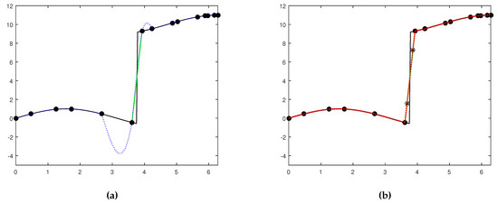
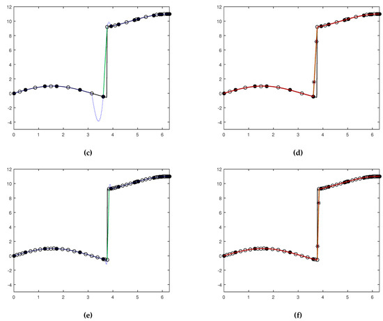
Figure 1. In black solid line: function $f\left(x\right)$, in green solid line the straight line joining the extreme points of the jump interval $[x_j^k,x_{j+1}^k],$ in blue dotted line: Lagrange reconstruction, in red dotted line: PPH reconstruction. Void circles stand for initial nodes, filled circles for nodes at the $k$ subdivision level and asterisks for points $P_1$ and $P_2$. (a) Lagrange $k=0,$ (b) PPH $k=0,$ (c) Lagrange $k=1,$ (d) PPH $k=1,$ (e) Lagrange $k=2,$ (f) PPH $k=2.$

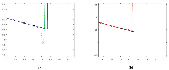
Figure 2. Zoom of the region around the jump discontinuity for subdivision grid level $k=3.$ (a) Lagrange, (b) $PPH.$

In the jump interval the distance $r_{max}^k$ decreases as $k$ increases, since $r_{max}^k=O\left(h^k\right).$ In Table 4 the values for $k=0,1,\dots ,7$ are shown. We can see that at a certain subdivision level the given values are approximately decreasing with the ratio $\frac{1}{2}.$ Therefore, PPH reconstruction approaches to the straight line $r_j^k\left(x\right)$ as $k$ increases.

Table 4. Distances $r_{max}^k$ obtained at subdivision level $k,k=0,1,2,3,4,5,6,7$.

	$\mathit{k}=0$	$\mathit{k}=1$	$\mathit{k}=2$	$\mathit{k}=3$	$\mathit{k}=4$	$\mathit{k}=5$	$\mathit{k}=6$	$\mathit{k}=7$
$r_{max}^k$	$1.1126\times {10}^{-3}$	$5.4822\times {10}^{-4}$	$1.2527\times {10}^{-3}$	$6.2825\times {10}^{-4}$	$3.1452\times {10}^{-4}$	$1.5735\times {10}^{-4}$	$7.8700\times {10}^{-5}$	$3.9356\times {10}^{-5}$

6. Conclusions

We have studied the behavior of the PPH reconstruction operator in presence of jump discontinuities for the case of working with $\sigma$ quasi-uniform grids. For this purpose, the arithmetic and harmonic means used in the uniform case are changed for weighted means with concrete weights, so that the main properties that allow for maintaining order of approximation in smooth areas and adaptation near singularities continue being true.

A explicit result concerning the approximation order, Theorem 1, has been proved, showing at least second order of approximation for the adjacent intervals to the one containing the jump discontinuity, and ensuring fourth order of approximation in convex (concave) parts of the function far from inflexion points. At a interval containing a inflexion point we get third order of approximation and in the vicinity the order grows progressively till fourth order.

A main result of this article is Theorem 2 in Section 4 proving that the presented reconstruction operator does not generate any Gibbs phenomena in the concrete sense indicated in the enunciate for $\sigma$ quasi-uniform grids where the maximum space between nodes of the grid is small enough.

Finally we have carried out some numerical experiments to reinforce the theoretical results proven as much in Proposition 1 as in Theorem 1.

References

- Amat, S.; Ruiz, J.; Shu, C.W. On a new WENO algorithm of order 2r with improved accuracy close to discontinuities. Appl. Math. Lett. 2020, 105, 106298–106309. [Google Scholar] [CrossRef]
- Amat, S.; Liandrat, J.; Ruiz, J.; Trillo, J.C. On a power WENO scheme with improved accuracy near discontinuities. SIAM J. Sci. Comput. 2017, 39, A2472–A2507. [Google Scholar] [CrossRef]
- Amir, A.; Levin, D. Quasi-interpolation and outliers removal. Numer. Algorithms 2018, 78, 805–825. [Google Scholar] [CrossRef]
- Aràndiga, F.; Donat, R.; Romani, L.; Rossini, M. On the reconstruction of discontinuous functions using multiquadric RBF-WENO local interpolation techniques. Math. Comput. Simul. 2020, 176, 4–24. [Google Scholar] [CrossRef]
- Harten, A. Eno schemes with subcell resolution. J. Comput. Phys. 1989, 83, 148–184. [Google Scholar] [CrossRef]
- Amat, S.; Magreñán, A.A.; Ruiz, J.; Trillo, J.C.; Yáñez, D.F. On the use of generalized harmonic means in image processing using multiresolution algorithms. Int. J. Comput. Math. 2020, 97, 455–466. [Google Scholar] [CrossRef]
- Donat, R.; Yáñez, D.F. A nonlinear Chaikin-based binary subdivision scheme. J. Comput. Appl. Math. 2019, 349, 379–389. [Google Scholar] [CrossRef]
- Dyn, N.; Farkhi, E.; Keinan, S. Approximation of 3D objects by piecewise linear geometric interpolants of their 1D cross-sections. J. Comput. Appl. Math. 2020, 368, 112466–112475. [Google Scholar] [CrossRef]
- Mateï, B.; Meignen, S. Nonlinear and nonseparable bidimensional multiscale representation based on cell-average representation. IEEE Trans. Image Process. 2015, 24, 4570–4580. [Google Scholar] [CrossRef]
- Dyn, N.; Gregori, J.A.; Levin, D. A 4-point interpolatory subdivision scheme for curve design. Comput. Aided Geom. Design 1987, 4, 257–268. [Google Scholar] [CrossRef]
- Dyn, N.; Kuijt, F.; Levin, D.; Van Damme, R. Convexity preservation of the four-point interpolatory subdivision scheme. Comput. Aided Geom. Design 1999, 16, 789–792. [Google Scholar] [CrossRef]
- Amat, S.; Donat, R.; Liandrat, J.; Trillo, J.C. Analysis of a new nonlinear subdivision scheme. Applications in image processing. Found. Comput. Math. 2006, 6, 193–225. [Google Scholar] [CrossRef]
- Amat, S.; Donat, R.; Trillo, J.C. Proving convexity preserving properties of interpolatory subdivision schemes through reconstruction operators. Appl. Math. Comput. 2013, 219, 7413–7421. [Google Scholar] [CrossRef]
- Trillo, J.C. Nonlinear Multiresolution and Applications in Image Processing. Ph.D. Thesis, University of Valencia, Valencia, Spain, 2007. [Google Scholar]
- Amat, S.; Dadourian, K.; Liandrat, J.; Trillo, J.C. High order nonlinear interpolatory reconstruction operators and associated multiresolution schemes. J. Comput. Appl. Math. 2013, 253, 163–180. [Google Scholar] [CrossRef]
- Amat, S.; Liandrat, J. On the stability of PPH nonlinear multiresolution. Appl. Comput. Harmon. Anal. 2005, 18, 198–206. [Google Scholar] [CrossRef]
- Floater, M.S.; Michelli, C.A. Nonlinear Stationary Subdivision. Approximation Theory. 1998, 212, 209–224. [Google Scholar]
- Kuijt, F.; Van Damme, R. Convexity preserving interpolatory subdivision schemes. Constr. Approx. 1998, 14, 609–630. [Google Scholar] [CrossRef]
- Dyn, N.; Levin, D. Stationary and non-stationary binary subdivision schemes. In Mathematical Methods in Computer Aided Geometric Design II; Academic Press: Boston, MA, USA, 1992; pp. 209–216. [Google Scholar]
- Aràndiga, F.; Donat, R. Nonlinear Multi-scale Decomposition: The Approach of A.Harten. Numer. Algorithms 2000, 23, 175–216. [Google Scholar] [CrossRef]
- Harten, A. Multiresolution representation of data II. SIAM J. Numer. Anal. 1996, 33, 1205–1256. [Google Scholar] [CrossRef]
- Ortiz, P.; Trillo, J.C. On the convexity preservation of a quasi C3 nonlinear interpolatory reconstruction operator on σ quasi-uniform grids. Mathematics 2021, 9, 310. [Google Scholar] [CrossRef]
- Amat, C.; Shu, C.W.; Ruiz, J.; Trillo, J.C. On a class of splines free of Gibbs phenomenon. Math. Modell. Numer. Anal. 2020. [Google Scholar] [CrossRef]
Publisher’s Note: MDPI stays neutral with regard to jurisdictional claims in published maps and institutional affiliations. |
© 2021 by the authors. Licensee MDPI, Basel, Switzerland. This article is an open access article distributed under the terms and conditions of the Creative Commons Attribution (CC BY) license (http://creativecommons.org/licenses/by/4.0/).