
A Multi-Strategy Marine Predator Algorithm and Its Application in Joint Regularization Semi-Supervised ELM


Abstract
1. Introduction
2. Marine Predator Algorithm and Its Improvement
2.1. Basic Marine Predator Algorithm
2.1.1. Population Location Initialization
2.1.2. Exploratory Phase of High-Speed Ratio
2.1.3. Mid-Speed Ratio Transition Phase
2.1.4. Low-Speed Ratio Development Phase
2.1.5. Eddy Current Formation and Fish Aggregation Device Effects (FADS)
2.2. Multi-Strategy Marine Predator Algorithm—MSMPA
2.2.1. Chaotic Opposition Learning Strategy
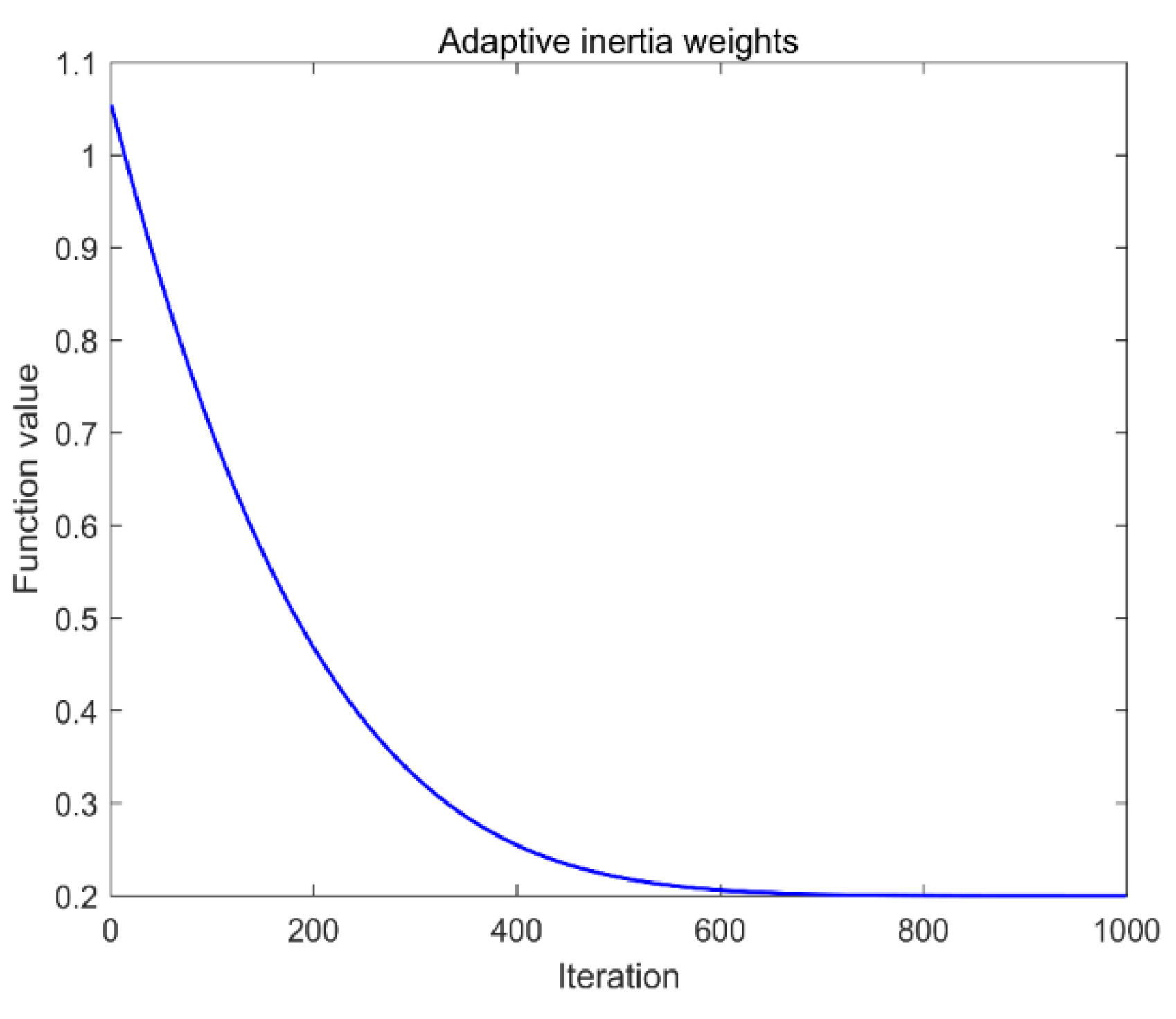
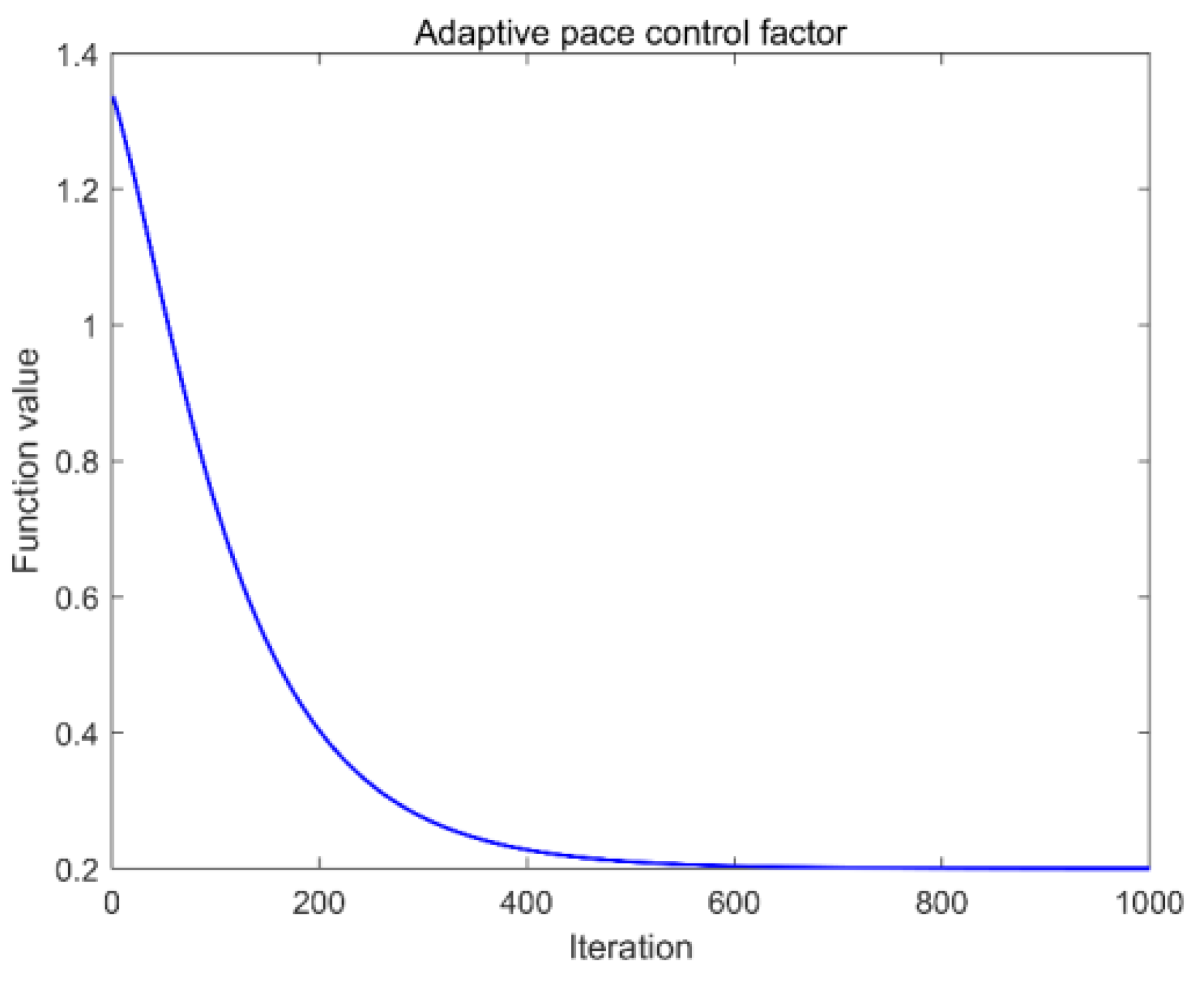
2.2.2. Adaptive Inertial Weights and Step Control Factors
2.2.3. Neighborhood Dimensional Learning Strategy (NDL)
| Algorithm 1: Pseudo-code of the MSMPA |
| Input: Number of Search Agents: N, Dim, Max_Iter |
| Output: The optimum fitness value |
| Generate chaotic tent mapping sequences by the Equation (11) |
| Initialized populations by the Equation (12) |
| Generation of Opposing Populations by the Equation (13) |
| Selection of the first N well-adapted individuals as the first generation of the population |
| While Iter < Max_Iter |
| Calculating Adaptive Inertia Weights by the Equation (14) |
| Calculating Adaptive Step Control Factors by the Equation (17) |
| Calculate fitness values and construct an elite matrix |
| If Iter < Max_Iter/3 |
| Update prey by the Equation (15) |
| Else if Max_Iter/3 < Iter < 2∗Max_Iter/3 |
| For the first half of the populations (i = 1, …, n/2) |
| Update prey by the Equation (15) |
| For the other half of the populations (i = n/2, …, n) |
| Update prey by the Equation (16) |
| Else if Iter > 2∗Max_Iter/3 |
| Update prey by the Equation (16) |
| End If |
| Generation of candidate populations by the Equation (18) |
| Calculating Neighborhood Radius by the Equation (19) |
| Finding Neighborhood Populations by the Equation (20) |
| Calculation of NDL populations by the Equation (21) |
| Calculate fitness values to update population position by the Equation (22) |
| Updating Memory and Applying FADs effect and update by the Equation (10) |
| Calculate the fitness value of the population by the fitness function |
| Update the current optimum fitness value and the position of the best Search Agent |
| End while |
| Return the optimum fitness value |
3. Simulation Experiments and Comparative Analysis
3.1. Experimental Environment and Algorithm Parameters
3.2. Benchmark Test Functions
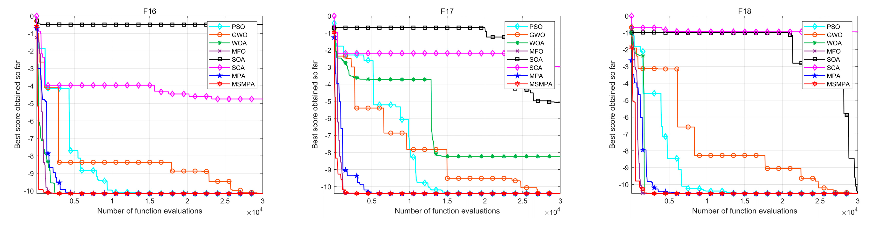
3.3. Experimental Results and Analysis
3.4. Algorithmic Stability Analysis
3.5. Wilcoxon Rank Sum Test Analysis
3.6. High-Dimensional Functional Test Analysis
4. Semi-Supervised Extreme Learning Machines and Its Improvements
4.1. Semi-Supervised Extreme Learning Machine
4.2. Joint Hessian and Supervised Information Regularization Semi-Supervised Extreme Learning Machine
4.2.1. Hessian Regularization
4.2.2. Supervisory Information Regularization
4.2.3. Joint Regularization SSELM
4.3. Hybrid MSMPA and Joint Regularized Semi-Supervised Extreme Learning Machine
| Algorithm 2. Pseudo-code of the MSMPA-JRSSELM |
| Input: L labeled samples |
| U unlabeled samples, |
| Number of Search Agents: N, Dim, Max_Iter |
| Output: The best mapping function of JRSSELM:f: |
| Step 1: Constructing Hessian regularization terms and supervisory information regularization terms via and . |
| Step 2: Generate chaotic tent mapping sequences by the Equation (11) |
| Initialized populations by the Equation (12) |
| Generation of Opposing Populations by the Equation (13) |
| Selection of the first N well-adapted individuals as the first generation of the population |
| Step 3: |
| If |
| Calculate the output weights by Equation (35) |
| Else if |
| Calculate the output weights by Equation (36) |
| Step 4: |
| While Iter < Max_Iter |
| Update all population positions by MSMPA |
| Repeat step 3 |
| Calculate the fitness of each search agent by the Equation (44) |
| End while |
| Step 5: Outputs the best search agent position and optimal value |
| Step 6: Optimal mapping functions of JLSSELM: |
5. Oil Logging Oil Layer Identification Applications
5.1. Design of Oil Layer Identification System
5.2. Practical Applications
6. Conclusions
Author Contributions
Funding
Data Availability Statement
Conflicts of Interest
Abbreviations
| ELM | Extreme Learning Machines |
| SSELM | Semi-Supervised Extreme Learning Machine |
| JRSSELM | Joint Regularized Semi-Supervised Extreme Learning Machine |
| MPA | Marine Predator Algorithm |
| MSMPA | Multi-Strategy Marine Predator Algorithm |
| PSO | Particle Swarm Optimization |
| GWO | Gray Wolf Optimization |
| MFO | Moth Flame Optimization |
| SOA | Seagull Optimization Algorithm |
| SCA | Sine Cosine Algorithm |
| WOA | Whale Optimization Algorithm |
| COA | Coyote Optimization Algorithm |
| CPA | Carnivorous Plant Algorithm |
| TSA | Transient Search Algorithm |
| RF | Random Forests |
| SVM | Support Vector Machines |
| LapSVM | Laplace Support Vector Machines |
| FADS | Fish Aggregation Device Effects |
| NDL | Neighborhood Dimensional Learning |
| GR | natural gamma |
| DT | acoustic time difference |
| SP | natural potential |
| LLD | deep lateral resistivity |
| LLS | shallow lateral resistivity |
| DEN | compensation density |
| K | Potassium |
| AC | acoustic time difference |
| RT | in situ ground resistivity |
| RXO | flush zone resistivity |
Appendix A


| Function | Criteria | MSMPA | MPA | PSO | GWO | WOA | MFO | SOA | SCA |
|---|---|---|---|---|---|---|---|---|---|
| F1 | Ave | 0.00 × 10+00 | 2.69 × 10−46 | 6.83 × 10+00 | 6.68 × 10−44 | 1.04 × 10−147 | 7.07 × 10+03 | 1.51 × 10⁻²⁰ | 2.49 × 10+02 |
| Std | 0.00 × 10+00 | 5.14 × 10−46 | 2.36 × 10+00 | 6.83 × 10−44 | 5.56 × 10−147 | 8.97 × 10+03 | 6.40 × 10⁻²⁰ | 4.54 × 10+02 | |
| Max | 0.00 × 10+00 | 2.51 × 10−45 | 1.32 × 10+01 | 2.82 × 10−43 | 3.10 × 10−146 | 3.00 × 10+04 | 3.58 × 10⁻¹⁹ | 2.10 × 10+03 | |
| Min | 0.00 × 10+00 | 8.73 × 10−50 | 2.58 × 10+00 | 1.17 × 10−45 | 7.10 × 10−169 | 5.58 × 10−01 | 8.03 × 10⁻²⁴ | 3.35 × 10−01 | |
| F2 | Ave | 0.00 × 10+00 | 1.54 × 10⁻²⁶ | 1.07 × 10+01 | 4.86 × 10⁻²⁶ | 1.53 × 10−102 | 7.23 × 10+01 | 5.22 × 10⁻¹⁴ | 3.62 × 10−02 |
| Std | 0.00 × 10+00 | 1.84 × 10⁻²⁶ | 1.99 × 10+00 | 7.31 × 10⁻²⁶ | 7.40 × 10−102 | 3.59 × 10+01 | 4.46 × 10⁻¹⁴ | 1.07 × 10−01 | |
| Max | 0.00 × 10+00 | 6.62 × 10⁻²⁶ | 1.43 × 10+01 | 4.06 × 10⁻²⁵ | 4.13 × 10−101 | 1.60 × 10+02 | 1.68 × 10⁻¹³ | 6.03 × 10−01 | |
| Min | 0.00 × 10+00 | 2.69 × 10⁻²⁹ | 6.18 × 10+00 | 6.58 × 10⁻²⁷ | 2.77 × 10−113 | 1.02 × 10+01 | 2.92 × 10⁻¹⁵ | 1.68 × 10−04 | |
| F3 | Ave | 0.00 × 10+00 | 1.41 × 10−07 | 1.14 × 10+03 | 4.79 × 10−05 | 1.26 × 10+05 | 5.10 × 10+04 | 5.27 × 10−08 | 3.40 × 10+04 |
| Std | 0.00 × 10+00 | 4.73 × 10−07 | 2.68 × 10+02 | 2.41 × 10−04 | 3.33 × 10+04 | 2.18 × 10+04 | 1.54 × 10−07 | 1.27 × 10+04 | |
| Max | 0.00 × 10+00 | 1.94 × 10−06 | 1.72 × 10+03 | 1.35 × 10−03 | 1.92 × 10+05 | 9.65 × 10+04 | 7.80 × 10−07 | 6.49 × 10+04 | |
| Min | 0.00 × 10+00 | 1.15 × 10⁻¹⁵ | 4.71 × 10+02 | 9.28 × 10⁻¹⁰ | 6.77 × 10+04 | 1.72 × 10+04 | 2.45 × 10⁻¹³ | 9.15 × 10+03 | |
| F4 | Ave | 0.00 × 10+00 | 1.34 × 10⁻¹⁷ | 3.27 × 10+00 | 1.54 × 10−09 | 6.31 × 10+01 | 8.44 × 10+01 | 2.51 × 10−01 | 5.97 × 10+01 |
| Std | 0.00 × 10+00 | 1.04 × 10⁻¹⁷ | 3.66 × 10−01 | 1.77 × 10−09 | 2.58 × 10+01 | 4.68 × 10+00 | 7.91 × 10−01 | 8.01 × 10+00 | |
| Max | 0.00 × 10+00 | 4.37 × 10⁻¹⁷ | 4.44 × 10+00 | 7.16 × 10−09 | 9.30 × 10+01 | 9.22 × 10+01 | 4.09 × 10+00 | 7.34 × 10+01 | |
| Min | 0.00 × 10+00 | 2.09 × 10⁻¹⁸ | 2.30 × 10+00 | 1.35 × 10⁻¹⁰ | 6.17 × 10+00 | 7.73 × 10+01 | 6.95 × 10−07 | 4.50 × 10+01 | |
| F5 | Ave | 7.20 × 10−06 | 4.44 × 10+01 | 3.46 × 10+03 | 4.73 × 10+01 | 4.77 × 10+01 | 1.34 × 10+07 | 4.84 × 10+01 | 6.32 × 10+05 |
| Std | 1.10 × 10−05 | 7.72 × 10−01 | 1.57 × 10+03 | 7.86 × 10−01 | 5.31 × 10−01 | 3.62 × 10+07 | 3.98 × 10−01 | 9.81 × 10+05 | |
| Max | 4.12 × 10−05 | 4.77 × 10+01 | 7.11 × 10+03 | 4.86 × 10+01 | 4.86 × 10+01 | 1.60 × 10+08 | 4.88 × 10+01 | 4.37 × 10+06 | |
| Min | 3.86 × 10⁻¹² | 4.32 × 10+01 | 1.32 × 10+03 | 4.61 × 10+01 | 4.67 × 10+01 | 4.03 × 10+02 | 4.72 × 10+01 | 4.06 × 10+03 | |
| F6 | Ave | 7.49 × 10−07 | 1.13 × 10−02 | 6.38 × 10+00 | 2.40 × 10+00 | 4.11 × 10−01 | 8.09 × 10+03 | 7.19 × 10+00 | 1.75 × 10+02 |
| Std | 9.73 × 10−07 | 4.31 × 10−02 | 2.08 × 10+00 | 5.60 × 10−01 | 2.24 × 10−01 | 9.11 × 10+03 | 5.36 × 10−01 | 3.22 × 10+02 | |
| Max | 3.87 × 10−06 | 2.16 × 10−01 | 1.25 × 10+01 | 3.25 × 10+00 | 1.04 × 10+00 | 4.02 × 10+04 | 8.13 × 10+00 | 1.22 × 10+03 | |
| Min | 1.05 × 10−08 | 3.24 × 10−08 | 3.04 × 10+00 | 1.25 × 10+00 | 8.74 × 10−02 | 1.08 × 10+00 | 5.89 × 10+00 | 8.70 × 10+00 | |
| F7 | Ave | 2.48 × 10−05 | 6.96 × 10−04 | 1.63 × 10+02 | 1.24 × 10−03 | 1.50 × 10−03 | 1.56 × 10+01 | 1.62 × 10−03 | 9.81 × 10−01 |
| Std | 1.95 × 10−05 | 3.03 × 10−04 | 6.65 × 10+01 | 6.62 × 10−04 | 1.77 × 10−03 | 1.87 × 10+01 | 1.59 × 10−03 | 1.29 × 10+00 | |
| Max | 8.65 × 10−05 | 1.17 × 10−03 | 3.12 × 10+02 | 2.75 × 10−03 | 7.74 × 10−03 | 7.84 × 10+01 | 7.56 × 10−03 | 5.10 × 10+00 | |
| Min | 8.50 × 10−07 | 1.76 × 10−04 | 4.01 × 10+01 | 4.42 × 10−04 | 2.61 × 10−06 | 4.46 × 10−01 | 2.76 × 10−04 | 2.77 × 10−02 | |
| F8 | Ave | −4.67 × 10+04 | −1.51 × 10+04 | −9.99 × 10+03 | −9.71 × 10+03 | −1.86 × 10+04 | −1.31 × 10+04 | −7.25 × 10+03 | −5.02 × 10+03 |
| Std | 1.12 × 10+04 | 6.77 × 10+02 | 2.01 × 10+03 | 8.12 × 10+02 | 2.60 × 10+03 | 1.27 × 10+03 | 1.09 × 10+03 | 3.08 × 10+02 | |
| Max | −1.85 × 10+04 | −1.39 × 10+04 | −4.30 × 10+03 | −8.11 × 10+03 | −1.32 × 10+04 | −1.10 × 10+04 | −5.82 × 10+03 | −4.61 × 10+03 | |
| Min | −5.45 × 10+04 | −1.63 × 10+04 | −1.25 × 10+04 | −1.12 × 10+04 | −2.09 × 10+04 | −1.51 × 10+04 | −1.00 × 10+04 | −5.68 × 10+03 | |
| F9 | Ave | 0.00 × 10+00 | 0.00 × 10+00 | 3.18 × 10+02 | 3.24 × 10−01 | 0.00 × 10+00 | 2.98 × 10+02 | 1.16 × 10−01 | 6.41 × 10+01 |
| Std | 0.00 × 10+00 | 0.00 × 10+00 | 4.37 × 10+01 | 1.39 × 10+00 | 0.00 × 10+00 | 6.59 × 10+01 | 6.23 × 10−01 | 4.72 × 10+01 | |
| Max | 0.00 × 10+00 | 0.00 × 10+00 | 4.11 × 10+02 | 7.48 × 10+00 | 0.00 × 10+00 | 4.26 × 10+02 | 3.47 × 10+00 | 1.74 × 10+02 | |
| Min | 0.00 × 10+00 | 0.00 × 10+00 | 2.25 × 10+02 | 0.00 × 10+00 | 0.00 × 10+00 | 1.73 × 10+02 | 0.00 × 10+00 | 1.32 × 10−01 | |
| F10 | Ave | 8.88 × 10⁻¹⁶ | 4.32 × 10⁻¹⁵ | 3.18 × 10+00 | 3.32 × 10⁻¹⁴ | 3.73 × 10⁻¹⁵ | 1.95 × 10+01 | 2.00 × 10+01 | 1.94 × 10+01 |
| Std | 0.00 × 10+00 | 6.38 × 10⁻¹⁶ | 3.72 × 10−01 | 4.71 × 10⁻¹⁵ | 2.81 × 10⁻¹⁵ | 5.73 × 10−01 | 9.30 × 10−04 | 3.73 × 10+00 | |
| Max | 8.88 × 10⁻¹⁶ | 4.44 × 10⁻¹⁵ | 4.04 × 10+00 | 4.35 × 10⁻¹⁴ | 7.99 × 10⁻¹⁵ | 2.00 × 10+01 | 2.00 × 10+01 | 2.05 × 10+01 | |
| Min | 8.88 × 10⁻¹⁶ | 8.88 × 10⁻¹⁶ | 2.49 × 10+00 | 2.22 × 10⁻¹⁴ | 8.88 × 10⁻¹⁶ | 1.76 × 10+01 | 2.00 × 10+01 | 9.91 × 10−02 | |
| F11 | Ave | 0.00 × 10+00 | 0.00 × 10+00 | 1.90 × 10−01 | 2.40 × 10−03 | 8.03 × 10−03 | 7.33 × 10+01 | 4.70 × 10−03 | 1.31 × 10+00 |
| Std | 0.00 × 10+00 | 0.00 × 10+00 | 7.04 × 10−02 | 7.28 × 10−03 | 2.42 × 10−02 | 7.82 × 10+01 | 1.35 × 10−02 | 7.09 × 10−01 | |
| Max | 0.00 × 10+00 | 0.00 × 10+00 | 4.10 × 10−01 | 2.71 × 10−02 | 8.76 × 10−02 | 2.71 × 10+02 | 6.16 × 10−02 | 4.82 × 10+00 | |
| Min | 0.00 × 10+00 | 0.00 × 10+00 | 9.82 × 10−02 | 0.00 × 10+00 | 0.00 × 10+00 | 7.64 × 10−01 | 0.00 × 10+00 | 6.90 × 10−01 | |
| F12 | Ave | 2.33 × 10−09 | 1.88 × 10−04 | 1.96 × 10−01 | 7.81 × 10−02 | 1.15 × 10−02 | 1.71 × 10+07 | 4.92 × 10−01 | 5.61 × 10+06 |
| Std | 2.83 × 10−09 | 6.10 × 10−04 | 3.31 × 10−01 | 2.68 × 10−02 | 7.35 × 10−03 | 6.39 × 10+07 | 1.00 × 10−01 | 1.42 × 10+07 | |
| Max | 1.42 × 10−08 | 2.96 × 10−03 | 1.88 × 10+00 | 1.54 × 10−01 | 3.48 × 10−02 | 2.56 × 10+08 | 7.93 × 10−01 | 7.01 × 10+07 | |
| Min | 2.10 × 10⁻¹² | 1.78 × 10−09 | 3.36 × 10−02 | 3.38 × 10−02 | 3.39 × 10−03 | 2.27 × 10+00 | 3.42 × 10−01 | 5.09 × 10+00 | |
| F13 | Ave | 4.59 × 10−08 | 9.99 × 10−02 | 1.96 × 10+00 | 1.92 × 10+00 | 6.35 × 10−01 | 4.10 × 10+07 | 3.95 × 10+00 | 3.43 × 10+06 |
| Std | 5.09 × 10−08 | 9.80 × 10−02 | 5.29 × 10−01 | 3.47 × 10−01 | 2.93 × 10−01 | 1.23 × 10+08 | 2.44 × 10−01 | 5.41 × 10+06 | |
| Max | 2.06 × 10−07 | 3.73 × 10−01 | 2.82 × 10+00 | 2.45 × 10+00 | 1.41 × 10+00 | 4.10 × 10+08 | 4.46 × 10+00 | 2.59 × 10+07 | |
| Min | 5.46 × 10⁻¹¹ | 8.88 × 10−08 | 1.14 × 10+00 | 7.63 × 10−01 | 1.92 × 10−01 | 2.27 × 10+01 | 3.54 × 10+00 | 6.89 × 10+02 | |
| F14 | Ave | 9.98 × 10−01 | 9.98 × 10−01 | 3.30 × 10+00 | 3.52 × 10+00 | 2.08 × 10+00 | 2.25 × 10+00 | 1.59 × 10+00 | 1.59 × 10+00 |
| Std | 0.00 × 10+00 | 5.73 × 10⁻¹⁷ | 2.67 × 10+00 | 3.54 × 10+00 | 2.45 × 10+00 | 2.10 × 10+00 | 9.09 × 10−01 | 9.08 × 10−01 | |
| Max | 9.98 × 10−01 | 9.98 × 10−01 | 1.08 × 10+01 | 1.27 × 10+01 | 1.08 × 10+01 | 1.08 × 10+01 | 2.98 × 10+00 | 2.98 × 10+00 | |
| Min | 9.98 × 10−01 | 9.98 × 10−01 | 9.98 × 10−01 | 9.98 × 10−01 | 9.98 × 10−01 | 9.98 × 10−01 | 9.98 × 10−01 | 9.98 × 10−01 | |
| F15 | Ave | 0.0004 | 0.0003 | 0.0008 | 0.0038 | 0.0007 | 0.001 | 0.0012 | 0.0009 |
| Std | 0.0002 | 0 | 0.0003 | 0.0074 | 0.0005 | 0.0004 | 0 | 0.0004 | |
| Max | 0.0012 | 0.0003 | 0.0019 | 0.0204 | 0.0022 | 0.0023 | 0.0012 | 0.0015 | |
| Min | 0.0003 | 0.0003 | 0.0004 | 0.0003 | 0.0003 | 0.0006 | 0.0012 | 0.0003 | |
| F16 | Ave | −10.1532 | −10.1532 | −7.7963 | −9.6475 | −8.6505 | −8.0628 | −3.5614 | −2.885 |
| Std | 0 | 0 | 2.7564 | 1.5157 | 2.5831 | 3.0377 | 4.3677 | 1.8174 | |
| Max | −10.1532 | −10.1532 | −2.6305 | −5.1003 | −0.881 | −2.6305 | −0.3507 | −0.4965 | |
| Min | −10.1532 | −10.1532 | −10.1532 | −10.1531 | −10.153 | −10.1532 | −10.1373 | −4.9475 | |
| F17 | Ave | −10.4028 | −10.4028 | −10.2258 | −10.2267 | −8.5934 | −8.7168 | −6.0807 | −4.1795 |
| Std | 0 | 0 | 0.9541 | 0.9467 | 2.7846 | 3.065 | 4.5085 | 2.4846 | |
| Max | −10.4028 | −10.4028 | −5.0877 | −5.1284 | −2.7655 | −2.7659 | −0.3724 | −0.5224 | |
| Min | −10.4028 | −10.4028 | −10.4028 | −10.4028 | −10.4028 | −10.4028 | −10.4005 | −9.5476 | |
| F18 | Ave | −10.5363 | −10.5363 | −9.8201 | −10.536 | −9.014 | −8.2934 | −8.0033 | −4.7824 |
| Std | 0 | 0 | 1.8263 | 0.0002 | 2.5492 | 3.225 | 3.938 | 1.5385 | |
| Max | −10.5363 | −10.5363 | −5.1285 | −10.5354 | −2.8064 | −2.4273 | −0.5542 | −0.9448 | |
| Min | −10.5363 | −10.5363 | −10.5363 | −10.5363 | −10.5363 | −10.5363 | −10.5342 | −8.8356 | |
| Friedman Average Rank | 1.6551 | 2.4101 | 4.9058 | 4.4775 | 4.3225 | 5.3986 | 5.7667 | 7.0638 | |
| Rank | 1 | 2 | 5 | 4 | 3 | 6 | 7 | 8 | |
| Function | Criteria | MSMPA | MPA | PSO | GWO | WOA | MFO | SOA | SCA |
|---|---|---|---|---|---|---|---|---|---|
| CF1 | Ave | 1.00 × 10+02 | 1.00 × 10+02 | 2.67 × 10+03 | 2.46 × 10+06 | 1.37 × 10+10 | 4.68 × 10+06 | 1.84 × 10+08 | 6.00 × 10+08 |
| Std | 1.58 × 10−05 | 6.00 × 10−03 | 2.86 × 10+03 | 6.44 × 10+06 | 5.50 × 10+09 | 1.75 × 10+07 | 1.83 × 10+08 | 2.07 × 10+08 | |
| CF2 | Ave | 2.00 × 10+02 | 2.00 × 10+02 | 2.00 × 10+02 | 3.68 × 10+06 | 1.57 × 10+12 | 1.04 × 10+08 | 1.29 × 10+07 | 7.48 × 10+06 |
| Std | 0.00 × 10+00 | 0.00 × 10+00 | 0.00 × 10+00 | 1.08 × 10+07 | 5.97 × 10+12 | 4.01 × 10+08 | 1.78 × 10+07 | 1.45 × 10+07 | |
| CF3 | Ave | 3.00 × 10+02 | 3.00 × 10+02 | 3.00 × 10+02 | 8.85 × 10+02 | 2.36 × 10+04 | 3.13 × 10+03 | 1.47 × 10+03 | 1.06 × 10+03 |
| Std | 4.01 × 10⁻¹⁰ | 2.83 × 10−08 | 2.29 × 10−08 | 1.15 × 10+03 | 1.33 × 10+04 | 4.97 × 10+03 | 1.08 × 10+03 | 4.75 × 10+02 | |
| CF4 | Ave | 4.00 × 10+02 | 4.00 × 10+02 | 4.03 × 10+02 | 4.12 × 10+02 | 1.50 × 10+03 | 4.09 × 10+02 | 4.40 × 10+02 | 4.33 × 10+02 |
| Std | 1.20 × 10−07 | 8.73 × 10−08 | 1.07 × 10+00 | 1.37 × 10+01 | 6.46 × 10+02 | 1.94 × 10+01 | 3.81 × 10+01 | 1.11 × 10+01 | |
| CF5 | Ave | 5.06 × 10+02 | 5.08 × 10+02 | 5.08 × 10+02 | 5.12 × 10+02 | 6.22 × 10+02 | 5.24 × 10+02 | 5.24 × 10+02 | 5.44 × 10+02 |
| Std | 2.00 × 10+00 | 2.36 × 10+00 | 3.43 × 10+00 | 4.20 × 10+00 | 2.05 × 10+01 | 8.03 × 10+00 | 8.55 × 10+00 | 5.94 × 10+00 | |
| CF6 | Ave | 6.00 × 10+02 | 6.00 × 10+02 | 6.00 × 10+02 | 6.00 × 10+02 | 6.74 × 10+02 | 6.00 × 10+02 | 6.08 × 10+02 | 6.16 × 10+02 |
| Std | 3.28 × 10−02 | 1.02 × 10−04 | 4.34 × 10⁻¹¹ | 7.31 × 10−01 | 1.50 × 10+01 | 9.98 × 10−01 | 4.30 × 10+00 | 3.22 × 10+00 | |
| CF7 | Ave | 7.12 × 10+02 | 7.19 × 10+02 | 7.17 × 10+02 | 7.26 × 10+02 | 9.65 × 10+02 | 7.35 × 10+02 | 7.53 × 10+02 | 7.70 × 10+02 |
| Std | 2.42 × 10+00 | 2.65 × 10+00 | 4.55 × 10+00 | 9.34 × 10+00 | 1.01 × 10+02 | 1.24 × 10+01 | 1.49 × 10+01 | 7.80 × 10+00 | |
| CF8 | Ave | 8.05 × 10+02 | 8.06 × 10+02 | 8.08 × 10+02 | 8.10 × 10+02 | 8.92 × 10+02 | 8.26 × 10+02 | 8.24 × 10+02 | 8.37 × 10+02 |
| Std | 2.27 × 10+00 | 1.98 × 10+00 | 3.04 × 10+00 | 4.00 × 10+00 | 1.98 × 10+01 | 1.21 × 10+01 | 6.17 × 10+00 | 5.99 × 10+00 | |
| CF9 | Ave | 9.00 × 10+02 | 9.00 × 10+02 | 9.00 × 10+02 | 9.04 × 10+02 | 2.74 × 10+03 | 9.38 × 10+02 | 9.84 × 10+02 | 9.72 × 10+02 |
| Std | 1.40 × 10−04 | 2.01 × 10−08 | 6.56 × 10⁻¹⁴ | 9.47 × 10+00 | 9.39 × 10+02 | 1.01 × 10+02 | 9.03 × 10+01 | 2.60 × 10+01 | |
| CF10 | Ave | 1.19 × 10+03 | 1.27 × 10+03 | 1.28 × 10+03 | 1.57 × 10+03 | 2.80 × 10+03 | 1.79 × 10+03 | 1.71 × 10+03 | 2.19 × 10+03 |
| Std | 1.19 × 10+02 | 9.66 × 10+01 | 1.23 × 10+02 | 2.44 × 10+02 | 1.70 × 10+02 | 3.19 × 10+02 | 2.22 × 10+02 | 1.99 × 10+02 | |
| CF11 | Ave | 1.10 × 10+03 | 1.10 × 10+03 | 1.10 × 10+03 | 1.13 × 10+03 | 5.46 × 10+03 | 1.13 × 10+03 | 1.20 × 10+03 | 1.19 × 10+03 |
| Std | 1.26 × 10+00 | 7.50 × 10−01 | 2.34 × 10+00 | 1.06 × 10+01 | 5.34 × 10+03 | 3.89 × 10+01 | 7.76 × 10+01 | 6.08 × 10+01 | |
| CF12 | Ave | 1.20 × 10+03 | 1.20 × 10+03 | 1.95 × 10+04 | 4.05 × 10+05 | 4.95 × 10+08 | 9.56 × 10+05 | 2.58 × 10+06 | 8.06 × 10+06 |
| Std | 1.68 × 10+01 | 5.14 × 10+00 | 1.91 × 10+04 | 5.72 × 10+05 | 4.98 × 10+08 | 2.16 × 10+06 | 2.43 × 10+06 | 6.55 × 10+06 | |
| CF13 | Ave | 1.30 × 10+03 | 1.30 × 10+03 | 5.92 × 10+03 | 1.07 × 10+04 | 3.07 × 10+07 | 1.17 × 10+04 | 1.67 × 10+04 | 2.28 × 10+04 |
| Std | 1.84 × 10+00 | 1.92 × 10+00 | 6.17 × 10+03 | 6.91 × 10+03 | 5.54 × 10+07 | 1.25 × 10+04 | 1.13 × 10+04 | 1.85 × 10+04 | |
| CF14 | Ave | 1.40 × 10+03 | 1.40 × 10+03 | 1.43 × 10+03 | 2.16 × 10+03 | 5.72 × 10+03 | 2.25 × 10+03 | 1.55 × 10+03 | 1.57 × 10+03 |
| Std | 1.95 × 10+00 | 2.07 × 10+00 | 1.10 × 10+01 | 1.40 × 10+03 | 8.46 × 10+03 | 9.25 × 10+02 | 6.39 × 10+01 | 5.21 × 10+01 | |
| CF15 | Ave | 1.50 × 10+03 | 1.50 × 10+03 | 1.53 × 10+03 | 3.10 × 10+03 | 2.09 × 10+04 | 4.43 × 10+03 | 2.26 × 10+03 | 2.09 × 10+03 |
| Std | 4.36 × 10−01 | 4.79 × 10−01 | 2.45 × 10+01 | 1.90 × 10+03 | 2.58 × 10+04 | 2.65 × 10+03 | 7.50 × 10+02 | 5.56 × 10+02 | |
| CF16 | Ave | 1.61 × 10+03 | 1.60 × 10+03 | 1.61 × 10+03 | 1.69 × 10+03 | 2.24 × 10+03 | 1.68 × 10+03 | 1.68 × 10+03 | 1.70 × 10+03 |
| Std | 2.97 × 10+01 | 4.22 × 10−01 | 3.35 × 10+01 | 5.79 × 10+01 | 2.38 × 10+02 | 9.95 × 10+01 | 7.44 × 10+01 | 5.33 × 10+01 | |
| CF17 | Ave | 1.71 × 10+03 | 1.71 × 10+03 | 1.71 × 10+03 | 1.75 × 10+03 | 2.01 × 10+03 | 1.74 × 10+03 | 1.77 × 10+03 | 1.77 × 10+03 |
| Std | 6.04 × 10+00 | 6.48 × 10+00 | 9.17 × 10+00 | 2.50 × 10+01 | 1.60 × 10+02 | 1.76 × 10+01 | 3.37 × 10+01 | 9.68 × 10+00 | |
| CF18 | Ave | 1.80 × 10+03 | 1.80 × 10+03 | 4.59 × 10+03 | 2.62 × 10+04 | 3.92 × 10+07 | 2.38 × 10+04 | 3.88 × 10+04 | 6.88 × 10+04 |
| Std | 1.41 × 10+00 | 1.17 × 10+00 | 2.47 × 10+03 | 1.43 × 10+04 | 7.49 × 10+07 | 1.82 × 10+04 | 1.08 × 10+04 | 3.97 × 10+04 | |
| CF19 | Ave | 1.90 × 10+03 | 1.90 × 10+03 | 1.92 × 10+03 | 4.64 × 10+03 | 8.76 × 10+05 | 8.04 × 10+03 | 7.50 × 10+03 | 2.68 × 10+03 |
| Std | 2.72 × 10−01 | 4.28 × 10−01 | 2.52 × 10+01 | 4.73 × 10+03 | 2.30 × 10+06 | 1.03 × 10+04 | 6.35 × 10+03 | 1.64 × 10+03 | |
| CF20 | Ave | 2.01 × 10+03 | 2.01 × 10+03 | 2.01 × 10+03 | 2.06 × 10+03 | 2.29 × 10+03 | 2.04 × 10+03 | 2.09 × 10+03 | 2.09 × 10+03 |
| Std | 4.48 × 10+00 | 8.41 × 10+00 | 1.06 × 10+01 | 4.01 × 10+01 | 7.52 × 10+01 | 2.26 × 10+01 | 5.71 × 10+01 | 2.08 × 10+01 | |
| CF21 | Ave | 2.24 × 10+03 | 2.20 × 10+03 | 2.29 × 10+03 | 2.30 × 10+03 | 2.35 × 10+03 | 2.27 × 10+03 | 2.20 × 10+03 | 2.23 × 10+03 |
| Std | 5.24 × 10+01 | 1.29 × 10−05 | 4.64 × 10+01 | 3.84 × 10+01 | 5.63 × 10+01 | 6.23 × 10+01 | 2.77 × 10+00 | 4.56 × 10+01 | |
| CF22 | Ave | 2.30 × 10+03 | 2.24 × 10+03 | 2.30 × 10+03 | 2.31 × 10+03 | 3.32 × 10+03 | 2.30 × 10+03 | 2.45 × 10+03 | 2.35 × 10+03 |
| Std | 1.84 × 10+01 | 4.78 × 10+01 | 1.51 × 10+01 | 4.85 × 10+00 | 4.75 × 10+02 | 2.19 × 10+01 | 3.61 × 10+02 | 1.83 × 10+01 | |
| CF23 | Ave | 2.51 × 10+03 | 2.58 × 10+03 | 2.61 × 10+03 | 2.61 × 10+03 | 2.73 × 10+03 | 2.63 × 10+03 | 2.63 × 10+03 | 2.65 × 10+03 |
| Std | 2.17 × 10+00 | 8.39 × 10+01 | 4.08 × 10+00 | 6.63 × 10+00 | 2.71 × 10+01 | 8.45 × 10+00 | 6.90 × 10+00 | 6.25 × 10+00 | |
| CF24 | Ave | 2.70 × 10+03 | 2.49 × 10+03 | 2.72 × 10+03 | 2.75 × 10+03 | 2.90 × 10+03 | 2.76 × 10+03 | 2.75 × 10+03 | 2.76 × 10+03 |
| Std | 7.88 × 10+01 | 2.49 × 10+01 | 5.98 × 10+01 | 1.03 × 10+01 | 6.38 × 10+01 | 9.34 × 10+00 | 9.90 × 10+00 | 6.77 × 10+01 | |
| CF25 | Ave | 2.91 × 10+03 | 2.86 × 10+03 | 2.92 × 10+03 | 2.93 × 10+03 | 4.01 × 10+03 | 2.93 × 10+03 | 2.94 × 10+03 | 2.95 × 10+03 |
| Std | 2.00 × 10+01 | 1.01 × 10+02 | 2.34 × 10+01 | 1.89 × 10+01 | 4.44 × 10+02 | 2.80 × 10+01 | 2.61 × 10+01 | 1.51 × 10+01 | |
| CF26 | Ave | 2.90 × 10+03 | 2.70 × 10+03 | 2.93 × 10+03 | 2.93 × 10+03 | 4.47 × 10+03 | 2.98 × 10+03 | 3.06 × 10+03 | 3.06 × 10+03 |
| Std | 2.44 × 10−04 | 1.05 × 10+02 | 1.69 × 10+02 | 1.78 × 10+02 | 3.99 × 10+02 | 5.46 × 10+01 | 2.37 × 10+02 | 2.22 × 10+01 | |
| CF27 | Ave | 3.08 × 10+03 | 3.09 × 10+03 | 3.10 × 10+03 | 3.09 × 10+03 | 3.26 × 10+03 | 3.09 × 10+03 | 3.09 × 10+03 | 3.10 × 10+03 |
| Std | 1.14 × 10+00 | 5.67 × 10−01 | 1.15 × 10+01 | 2.90 × 10+00 | 6.07 × 10+01 | 1.95 × 10+00 | 1.91 × 10+00 | 1.90 × 10+00 | |
| CF28 | Ave | 3.11 × 10+03 | 3.07 × 10+03 | 3.23 × 10+03 | 3.35 × 10+03 | 3.69 × 10+03 | 3.25 × 10+03 | 3.23 × 10+03 | 3.25 × 10+03 |
| Std | 3.23 × 10+01 | 9.00 × 10+01 | 1.59 × 10+02 | 8.68 × 10+01 | 1.15 × 10+02 | 8.01 × 10+01 | 8.22 × 10+01 | 5.64 × 10+01 | |
| CF29 | Ave | 3.14 × 10+03 | 3.13 × 10+03 | 3.16 × 10+03 | 3.17 × 10+03 | 3.58 × 10+03 | 3.20 × 10+03 | 3.18 × 10+03 | 3.21 × 10+03 |
| Std | 7.29 × 10+00 | 9.20 × 10+00 | 1.90 × 10+01 | 1.98 × 10+01 | 1.34 × 10+02 | 4.05 × 10+01 | 2.57 × 10+01 | 2.17 × 10+01 | |
| CF30 | Ave | 3.31 × 10+03 | 3.40 × 10+03 | 6.02 × 10+05 | 5.65 × 10+05 | 1.23 × 10+07 | 5.64 × 10+05 | 7.35 × 10+04 | 6.44 × 10+05 |
| Std | 3.66 × 10+01 | 4.54 × 10+00 | 8.68 × 10+05 | 6.42 × 10+05 | 1.03 × 10+07 | 5.53 × 10+05 | 1.25 × 10+05 | 4.64 × 10+05 | |
| Friedman Average Rank | 1.6167 | 2.4489 | 2.9056 | 4.6561 | 7.9300 | 4.7728 | 5.3978 | 6.2722 | |
| Rank | 1 | 2 | 3 | 4 | 8 | 5 | 6 | 7 | |
| Function | MSMPA VS. | |||||||
|---|---|---|---|---|---|---|---|---|
| MPA | PSO | GWO | WOA | MFO | SOA | SCA | ||
| F1 | p-value | 1.21 × 10⁻¹² | 1.21 × 10⁻¹² | 1.21 × 10⁻¹² | 1.21 × 10⁻¹² | 1.21 × 10⁻¹² | 1.21 × 10⁻¹² | 1.21 × 10⁻¹² |
| F2 | p-value | 1.21 × 10⁻¹² | 1.21 × 10⁻¹² | 1.21 × 10⁻¹² | 1.21 × 10⁻¹² | 1.21 × 10⁻¹² | 1.21 × 10⁻¹² | 1.21 × 10⁻¹² |
| F3 | p-value | 1.21 × 10⁻¹² | 1.21 × 10⁻¹² | 1.21 × 10⁻¹² | 1.21 × 10⁻¹² | 1.21 × 10⁻¹² | 1.21 × 10⁻¹² | 1.21 × 10⁻¹² |
| F4 | p-value | 1.21 × 10⁻¹² | 1.21 × 10⁻¹² | 1.21 × 10⁻¹² | 1.21 × 10⁻¹² | 1.21 × 10⁻¹² | 1.21 × 10⁻¹² | 1.21 × 10⁻¹² |
| F5 | p-value | 3.02 × 10⁻¹¹ | 3.02 × 10⁻¹¹ | 3.02 × 10⁻¹¹ | 3.02 × 10⁻¹¹ | 3.02 × 10⁻¹¹ | 3.02 × 10⁻¹¹ | 3.02 × 10⁻¹¹ |
| F6 | p-value | 8.56 × 10−04 | 3.02 × 10⁻¹¹ | 3.02 × 10⁻¹¹ | 3.02 × 10⁻¹¹ | 3.02 × 10⁻¹¹ | 3.02 × 10⁻¹¹ | 3.02 × 10⁻¹¹ |
| F7 | p-value | 3.02 × 10⁻¹¹ | 3.02 × 10⁻¹¹ | 3.02 × 10⁻¹¹ | 1.07 × 10−09 | 3.02 × 10⁻¹¹ | 3.02 × 10⁻¹¹ | 3.02 × 10⁻¹¹ |
| F8 | p-value | 3.02 × 10⁻¹¹ | 3.02 × 10⁻¹¹ | 3.02 × 10⁻¹¹ | 8.10 × 10⁻¹⁰ | 3.02 × 10⁻¹¹ | 3.02 × 10⁻¹¹ | 3.02 × 10⁻¹¹ |
| F9 | p-value | NaN | 1.21 × 10⁻¹² | 1.14 × 10−05 | NaN | 1.21 × 10⁻¹² | 2.79 × 10−03 | 1.21 × 10⁻¹² |
| F10 | p-value | 1.17 × 10⁻¹³ | 1.21 × 10⁻¹² | 8.56 × 10⁻¹³ | 1.97 × 10−06 | 1.21 × 10⁻¹² | 1.21 × 10⁻¹² | 1.21 × 10⁻¹² |
| F11 | p-value | NaN | 1.21 × 10⁻¹² | 8.15 × 10−02 | 8.15 × 10−02 | 1.21 × 10⁻¹² | 5.58 × 10−03 | 1.21 × 10⁻¹² |
| F12 | p-value | 1.25 × 10−07 | 3.02 × 10⁻¹¹ | 3.02 × 10⁻¹¹ | 3.02 × 10⁻¹¹ | 3.02 × 10⁻¹¹ | 3.02 × 10⁻¹¹ | 3.02 × 10⁻¹¹ |
| F13 | p-value | 8.15 × 10⁻¹¹ | 3.02 × 10⁻¹¹ | 3.02 × 10⁻¹¹ | 3.02 × 10⁻¹¹ | 3.02 × 10⁻¹¹ | 3.02 × 10⁻¹¹ | 3.02 × 10⁻¹¹ |
| F14 | p-value | 1.61 × 10−01 | 4.42 × 10−08 | 1.21 × 10⁻¹² | 1.21 × 10⁻¹² | 2.90 × 10−05 | 1.21 × 10⁻¹² | 1.21 × 10⁻¹² |
| F15 | p-value | 1.05 × 10−05 | 6.59 × 10−09 | 1.30 × 10−09 | 2.69 × 10−09 | 1.08 × 10−09 | 2.73 × 10⁻¹¹ | 1.30 × 10−09 |
| F16 | p-value | 3.49 × 10−04 | 1.38 × 10−09 | 8.87 × 10⁻¹² | 8.87 × 10⁻¹² | 2.04 × 10−01 | 8.87 × 10⁻¹² | 8.87 × 10⁻¹² |
| F17 | p-value | 4.18 × 10−02 | 3.03 × 10−03 | 4.08 × 10⁻¹² | 4.08 × 10⁻¹² | 5.20 × 10−02 | 4.08 × 10⁻¹² | 4.08 × 10⁻¹² |
| F18 | p-value | 2.85 × 10−05 | 1.22 × 10−09 | 4.08 × 10⁻¹² | 4.08 × 10⁻¹² | 3.40 × 10−02 | 4.08 × 10⁻¹² | 4.08 × 10⁻¹² |
| CF1 | p-value | 3.02 × 10⁻¹¹ | 3.02 × 10⁻¹¹ | 3.02 × 10⁻¹¹ | 3.02 × 10⁻¹¹ | 2.95 × 10⁻¹¹ | 3.02 × 10⁻¹¹ | 3.02 × 10⁻¹¹ |
| CF2 | p-value | NaN | NaN | 4.57 × 10⁻¹² | 1.21 × 10⁻¹² | 5.60 × 10⁻¹¹ | 1.21 × 10⁻¹² | 1.21 × 10⁻¹² |
| CF3 | p-value | 3.02 × 10⁻¹¹ | 3.50 × 10−03 | 3.02 × 10⁻¹¹ | 3.02 × 10⁻¹¹ | 8.77 × 10−01 | 3.02 × 10⁻¹¹ | 3.02 × 10⁻¹¹ |
| CF4 | p-value | 1.09 × 10−01 | 3.02 × 10⁻¹¹ | 3.02 × 10⁻¹¹ | 3.02 × 10⁻¹¹ | 2.86 × 10⁻¹¹ | 3.02 × 10⁻¹¹ | 3.02 × 10⁻¹¹ |
| CF5 | p-value | 1.06 × 10−03 | 5.82 × 10−03 | 1.25 × 10−07 | 3.02 × 10⁻¹¹ | 3.02 × 10⁻¹¹ | 4.62 × 10⁻¹⁰ | 3.02 × 10⁻¹¹ |
| CF6 | p-value | 3.02 × 10⁻¹¹ | 9.37 × 10⁻¹² | 9.35 × 10−01 | 3.02 × 10⁻¹¹ | 3.46 × 10−04 | 3.02 × 10⁻¹¹ | 3.02 × 10⁻¹¹ |
| CF7 | p-value | 5.86 × 10−06 | 1.87 × 10−05 | 5.49 × 10−01 | 3.02 × 10⁻¹¹ | 2.57 × 10−07 | 3.02 × 10⁻¹¹ | 3.02 × 10⁻¹¹ |
| CF8 | p-value | 6.35 × 10−02 | 5.94 × 10−05 | 1.25 × 10−07 | 3.02 × 10⁻¹¹ | 2.15 × 10⁻¹⁰ | 3.02 × 10⁻¹¹ | 3.02 × 10⁻¹¹ |
| CF9 | p-value | 3.02 × 10⁻¹¹ | 1.14 × 10⁻¹¹ | 3.02 × 10⁻¹¹ | 3.02 × 10⁻¹¹ | 7.26 × 10−02 | 3.02 × 10⁻¹¹ | 3.02 × 10⁻¹¹ |
| CF10 | p-value | 1.38 × 10−02 | 2.32 × 10−02 | 7.12 × 10−09 | 3.02 × 10⁻¹¹ | 8.99 × 10⁻¹¹ | 4.97 × 10⁻¹¹ | 3.02 × 10⁻¹¹ |
| CF11 | p-value | 2.03 × 10−07 | 7.96 × 10−01 | 4.50 × 10⁻¹¹ | 3.02 × 10⁻¹¹ | 7.09 × 10−08 | 3.02 × 10⁻¹¹ | 3.02 × 10⁻¹¹ |
| CF12 | p-value | 3.02 × 10⁻¹¹ | 3.02 × 10⁻¹¹ | 3.02 × 10⁻¹¹ | 3.02 × 10⁻¹¹ | 3.02 × 10⁻¹¹ | 3.02 × 10⁻¹¹ | 3.02 × 10⁻¹¹ |
| CF13 | p-value | 1.56 × 10−08 | 9.92 × 10⁻¹¹ | 3.02 × 10⁻¹¹ | 3.02 × 10⁻¹¹ | 3.02 × 10⁻¹¹ | 3.02 × 10⁻¹¹ | 3.02 × 10⁻¹¹ |
| CF14 | p-value | 7.77 × 10−09 | 2.02 × 10−08 | 3.02 × 10⁻¹¹ | 3.02 × 10⁻¹¹ | 3.02 × 10⁻¹¹ | 3.02 × 10⁻¹¹ | 3.02 × 10⁻¹¹ |
| CF15 | p-value | 4.69 × 10−08 | 6.70 × 10⁻¹¹ | 3.02 × 10⁻¹¹ | 3.02 × 10⁻¹¹ | 3.02 × 10⁻¹¹ | 3.02 × 10⁻¹¹ | 3.02 × 10⁻¹¹ |
| CF16 | p-value | 4.42 × 10−06 | 2.68 × 10−06 | 6.72 × 10⁻¹⁰ | 3.34 × 10⁻¹¹ | 3.96 × 10−08 | 8.10 × 10⁻¹⁰ | 4.20 × 10⁻¹⁰ |
| CF17 | p-value | 3.82 × 10−09 | 1.04 × 10−04 | 1.33 × 10⁻¹⁰ | 3.02 × 10⁻¹¹ | 4.80 × 10−07 | 4.08 × 10⁻¹¹ | 3.02 × 10⁻¹¹ |
| CF18 | p-value | 1.60 × 10−07 | 3.02 × 10⁻¹¹ | 3.02 × 10⁻¹¹ | 3.02 × 10⁻¹¹ | 3.02 × 10⁻¹¹ | 3.02 × 10⁻¹¹ | 3.02 × 10⁻¹¹ |
| CF19 | p-value | 3.02 × 10⁻¹¹ | 4.50 × 10⁻¹¹ | 3.02 × 10⁻¹¹ | 3.02 × 10⁻¹¹ | 3.02 × 10⁻¹¹ | 3.02 × 10⁻¹¹ | 3.02 × 10⁻¹¹ |
| CF20 | p-value | 2.90 × 10−01 | 5.59 × 10−01 | 4.50 × 10⁻¹¹ | 3.02 × 10⁻¹¹ | 1.07 × 10−07 | 3.02 × 10⁻¹¹ | 3.02 × 10⁻¹¹ |
| CF21 | p-value | 4.29 × 10−01 | 1.41 × 10−04 | 2.38 × 10−07 | 4.11 × 10−07 | 3.99 × 10−04 | 1.86 × 10−01 | 4.21 × 10−02 |
| CF22 | p-value | 1.78 × 10⁻¹⁰ | 1.68 × 10−04 | 1.00 × 10−03 | 3.02 × 10⁻¹¹ | 1.62 × 10−01 | 6.74 × 10−06 | 5.07 × 10⁻¹⁰ |
| CF23 | p-value | 2.12 × 10−01 | 3.63 × 10−01 | 2.15 × 10−06 | 3.02 × 10⁻¹¹ | 3.34 × 10⁻¹¹ | 3.34 × 10⁻¹¹ | 3.02 × 10⁻¹¹ |
| CF24 | p-value | 4.62 × 10⁻¹⁰ | 4.11 × 10−07 | 9.76 × 10⁻¹⁰ | 1.96 × 10⁻¹⁰ | 3.02 × 10⁻¹¹ | 8.89 × 10⁻¹⁰ | 3.96 × 10−08 |
| CF25 | p-value | 4.50 × 10⁻¹¹ | 2.77 × 10−05 | 7.60 × 10−07 | 3.02 × 10⁻¹¹ | 1.39 × 10−06 | 7.66 × 10−05 | 4.11 × 10−07 |
| CF26 | p-value | 2.61 × 10⁻¹⁰ | 6.44 × 10−09 | 8.48 × 10−09 | 3.02 × 10⁻¹¹ | 9.47 × 10−06 | 3.02 × 10⁻¹¹ | 3.02 × 10⁻¹¹ |
| CF27 | p-value | 3.02 × 10⁻¹¹ | 3.02 × 10⁻¹¹ | 3.02 × 10⁻¹¹ | 3.02 × 10⁻¹¹ | 3.02 × 10⁻¹¹ | 3.02 × 10⁻¹¹ | 3.02 × 10⁻¹¹ |
| CF28 | p-value | 1.67 × 10−01 | 3.04 × 10−01 | 9.92 × 10⁻¹¹ | 3.02 × 10⁻¹¹ | 4.59 × 10⁻¹⁰ | 2.92 × 10−09 | 3.02 × 10⁻¹¹ |
| CF29 | p-value | 3.03 × 10−03 | 1.17 × 10−05 | 5.00 × 10−09 | 3.02 × 10⁻¹¹ | 7.38 × 10⁻¹⁰ | 5.07 × 10⁻¹⁰ | 3.02 × 10⁻¹¹ |
| CF30 | p-value | 3.02 × 10⁻¹¹ | 3.02 × 10⁻¹¹ | 3.02 × 10⁻¹¹ | 3.02 × 10⁻¹¹ | 3.02 × 10⁻¹¹ | 3.02 × 10⁻¹¹ | 3.01 × 10⁻¹¹ |
| Function | Criteria | MSMPA | MPA | PSO | GWO | WOA | MFO | SOA | SCA |
|---|---|---|---|---|---|---|---|---|---|
| F1 | Ave | 0.00 × 10+00 | 3.85 × 10−43 | 9.41 × 10+01 | 1.84 × 10⁻²⁹ | 7.06 × 10−146 | 3.17 × 10+04 | 6.07 × 10⁻¹⁵ | 5.59 × 10+03 |
| Std | 0.00 × 10+00 | 3.58 × 10−43 | 1.46 × 10+01 | 1.73 × 10⁻²⁹ | 3.80 × 10−145 | 1.25 × 10+04 | 1.14 × 10⁻¹⁴ | 4.77 × 10+03 | |
| Max | 0.00 × 10+00 | 1.50 × 10−42 | 1.37 × 10+02 | 6.52 × 10⁻²⁹ | 2.12 × 10−144 | 5.46 × 10+04 | 4.98 × 10⁻¹⁴ | 1.91 × 10+04 | |
| Min | 0.00 × 10+00 | 2.21 × 10−44 | 7.18 × 10+01 | 4.12 × 10⁻³⁰ | 2.81 × 10−169 | 1.43 × 10+04 | 1.68 × 10⁻¹⁷ | 2.73 × 10+01 | |
| F2 | Ave | 0.00 × 10+00 | 8.27 × 10⁻²⁵ | 1.10 × 10+02 | 5.34 × 10⁻¹⁸ | 3.13 × 10−101 | 1.79 × 10+02 | 8.13 × 10⁻¹¹ | 1.99 × 10+00 |
| Std | 0.00 × 10+00 | 1.44 × 10⁻²⁴ | 2.24 × 10+01 | 3.05 × 10⁻¹⁸ | 1.63 × 10−100 | 5.48 × 10+01 | 6.58 × 10⁻¹¹ | 2.27 × 10+00 | |
| Max | 0.00 × 10+00 | 6.14 × 10⁻²⁴ | 1.71 × 10+02 | 1.66 × 10⁻¹⁷ | 9.06 × 10−100 | 3.30 × 10+02 | 2.30 × 10⁻¹⁰ | 9.10 × 10+00 | |
| Min | 0.00 × 10+00 | 2.27 × 10⁻²⁷ | 6.46 × 10+01 | 2.06 × 10⁻¹⁸ | 1.63 × 10−110 | 1.03 × 10+02 | 5.48 × 10⁻¹² | 8.84 × 10−02 | |
| F3 | Ave | 0.00 × 10+00 | 2.49 × 10−02 | 1.39 × 10+04 | 1.06 × 10+01 | 8.92 × 10+05 | 1.80 × 10+05 | 2.11 × 10−02 | 1.92 × 10+05 |
| Std | 0.00 × 10+00 | 9.79 × 10−02 | 2.69 × 10+03 | 2.70 × 10+01 | 2.40 × 10+05 | 4.35 × 10+04 | 8.57 × 10−02 | 4.22 × 10+04 | |
| Max | 0.00 × 10+00 | 5.42 × 10−01 | 2.00 × 10+04 | 1.41 × 10+02 | 1.45 × 10+06 | 2.80 × 10+05 | 4.77 × 10−01 | 2.93 × 10+05 | |
| Min | 0.00 × 10+00 | 1.13 × 10−07 | 1.00 × 10+04 | 2.38 × 10−02 | 4.91 × 10+05 | 1.04 × 10+05 | 3.52 × 10−07 | 1.12 × 10+05 | |
| F4 | Ave | 0.00 × 10+00 | 5.90 × 10⁻¹⁶ | 1.03 × 10+01 | 1.60 × 10−02 | 7.20 × 10+01 | 9.32 × 10+01 | 5.60 × 10+01 | 8.66 × 10+01 |
| Std | 0.00 × 10+00 | 3.81 × 10⁻¹⁶ | 1.03 × 10+00 | 7.52 × 10−02 | 2.86 × 10+01 | 1.78 × 10+00 | 2.47 × 10+01 | 3.84 × 10+00 | |
| Max | 0.00 × 10+00 | 1.88 × 10⁻¹⁵ | 1.25 × 10+01 | 4.21 × 10−01 | 9.62 × 10+01 | 9.60 × 10+01 | 8.51 × 10+01 | 9.34 × 10+01 | |
| Min | 0.00 × 10+00 | 1.52 × 10⁻¹⁶ | 8.46 × 10+00 | 3.78 × 10−05 | 1.10 × 10−04 | 8.84 × 10+01 | 3.28 × 10+00 | 7.87 × 10+01 | |
| F5 | Ave | 2.25 × 10−05 | 9.57 × 10+01 | 1.04 × 10+05 | 9.76 × 10+01 | 9.78 × 10+01 | 6.84 × 10+07 | 9.86 × 10+01 | 5.17 × 10+07 |
| Std | 3.40 × 10−05 | 1.11 × 10+00 | 3.00 × 10+04 | 6.31 × 10−01 | 4.12 × 10−01 | 5.92 × 10+07 | 1.90 × 10−01 | 3.00 × 10+07 | |
| Max | 1.32 × 10−04 | 9.78 × 10+01 | 2.10 × 10+05 | 9.85 × 10+01 | 9.83 × 10+01 | 2.62 × 10+08 | 9.88 × 10+01 | 1.21 × 10+08 | |
| Min | 7.28 × 10⁻¹⁵ | 9.41 × 10+01 | 6.35 × 10+04 | 9.61 × 10+01 | 9.70 × 10+01 | 3.05 × 10+06 | 9.80 × 10+01 | 1.04 × 10+07 | |
| F6 | Ave | 1.45 × 10−05 | 9.22 × 10−01 | 1.00 × 10+02 | 9.29 × 10+00 | 2.08 × 10+00 | 3.19 × 10+04 | 1.83 × 10+01 | 6.73 × 10+03 |
| Std | 4.13 × 10−05 | 4.35 × 10−01 | 1.87 × 10+01 | 8.26 × 10−01 | 7.60 × 10−01 | 1.34 × 10+04 | 7.55 × 10−01 | 4.69 × 10+03 | |
| Max | 2.25 × 10−04 | 1.82 × 10+00 | 1.40 × 10+02 | 1.09 × 10+01 | 4.49 × 10+00 | 5.75 × 10+04 | 1.97 × 10+01 | 1.78 × 10+04 | |
| Min | 1.85 × 10−08 | 1.03 × 10−01 | 7.24 × 10+01 | 7.69 × 10+00 | 1.03 × 10+00 | 5.68 × 10+03 | 1.66 × 10+01 | 1.57 × 10+02 | |
| F7 | Ave | 3.26 × 10−05 | 7.46 × 10−04 | 1.41 × 10+03 | 2.48 × 10−03 | 2.60 × 10−03 | 1.81 × 10+02 | 2.95 × 10−03 | 6.74 × 10+01 |
| Std | 2.41 × 10−05 | 3.55 × 10−04 | 2.64 × 10+02 | 7.68 × 10−04 | 2.09 × 10−03 | 1.27 × 10+02 | 1.82 × 10−03 | 3.73 × 10+01 | |
| Max | 1.05 × 10−04 | 2.00 × 10−03 | 2.07 × 10+03 | 4.45 × 10−03 | 7.12 × 10−03 | 5.70 × 10+02 | 7.85 × 10−03 | 1.55 × 10+02 | |
| Min | 1.16 × 10−06 | 3.16 × 10−04 | 9.92 × 10+02 | 1.29 × 10−03 | 7.26 × 10−05 | 4.24 × 10+01 | 3.40 × 10−04 | 8.02 × 10+00 | |
| F8 | Ave | −1.02 × 10+05 | −2.76 × 10+04 | −2.14 × 10+04 | −1.59 × 10+04 | −3.77 × 10+04 | −2.34 × 10+04 | −1.12 × 10+04 | −7.30 × 10+03 |
| Std | 1.36 × 10+04 | 9.19 × 10+02 | 3.47 × 10+03 | 2.36 × 10+03 | 4.85 × 10+03 | 1.94 × 10+03 | 1.49 × 10+03 | 5.79 × 10+02 | |
| Max | −3.73 × 10+04 | −2.56 × 10+04 | −7.61 × 10+03 | −5.92 × 10+03 | −2.87 × 10+04 | −2.04 × 10+04 | −8.71 × 10+03 | −6.30 × 10+03 | |
| Min | −1.09 × 10+05 | −2.99 × 10+04 | −2.65 × 10+04 | −2.01 × 10+04 | −4.19 × 10+04 | −2.75 × 10+04 | −1.48 × 10+04 | −8.72 × 10+03 | |
| F9 | Ave | 0.00 × 10+00 | 0.00 × 10+00 | 1.10 × 10+03 | 3.57 × 10−01 | 7.58 × 10⁻¹⁵ | 7.61 × 10+02 | 2.10 × 10⁻¹² | 2.45 × 10+02 |
| Std | 0.00 × 10+00 | 0.00 × 10+00 | 1.06 × 10+02 | 1.00 × 10+00 | 4.08 × 10⁻¹⁴ | 7.43 × 10+01 | 8.14 × 10⁻¹² | 9.94 × 10+01 | |
| Max | 0.00 × 10+00 | 0.00 × 10+00 | 1.27 × 10+03 | 3.92 × 10+00 | 2.27 × 10⁻¹³ | 9.24 × 10+02 | 4.48 × 10⁻¹¹ | 4.81 × 10+02 | |
| Min | 0.00 × 10+00 | 0.00 × 10+00 | 8.67 × 10+02 | 0.00 × 10+00 | 0.00 × 10+00 | 5.95 × 10+02 | 0.00 × 10+00 | 5.70 × 10+01 | |
| F10 | Ave | 8.88 × 10⁻¹⁶ | 4.44 × 10⁻¹⁵ | 5.45 × 10+00 | 1.12 × 10⁻¹³ | 3.73 × 10⁻¹⁵ | 1.98 × 10+01 | 2.00 × 10+01 | 1.93 × 10+01 |
| Std | 0.00 × 10+00 | 0.00 × 10+00 | 2.94 × 10−01 | 1.09 × 10⁻¹⁴ | 2.66 × 10⁻¹⁵ | 2.26 × 10−01 | 2.26 × 10−04 | 3.81 × 10+00 | |
| Max | 8.88 × 10⁻¹⁶ | 4.44 × 10⁻¹⁵ | 5.93 × 10+00 | 1.47 × 10⁻¹³ | 7.99 × 10⁻¹⁵ | 2.00 × 10+01 | 2.00 × 10+01 | 2.07 × 10+01 | |
| Min | 8.88 × 10⁻¹⁶ | 4.44 × 10⁻¹⁵ | 4.71 × 10+00 | 9.33 × 10⁻¹⁴ | 8.88 × 10⁻¹⁶ | 1.92 × 10+01 | 2.00 × 10+01 | 5.48 × 10+00 | |
| F11 | Ave | 0.00 × 10+00 | 0.00 × 10+00 | 7.96 × 10−01 | 3.16 × 10−03 | 3.78 × 10−03 | 2.98 × 10+02 | 5.27 × 10−03 | 4.75 × 10+01 |
| Std | 0.00 × 10+00 | 0.00 × 10+00 | 7.24 × 10−02 | 6.69 × 10−03 | 2.03 × 10−02 | 1.28 × 10+02 | 1.77 × 10−02 | 3.63 × 10+01 | |
| Max | 0.00 × 10+00 | 0.00 × 10+00 | 9.26 × 10−01 | 2.59 × 10−02 | 1.13 × 10−01 | 5.81 × 10+02 | 8.51 × 10−02 | 1.27 × 10+02 | |
| Min | 0.00 × 10+00 | 0.00 × 10+00 | 6.41 × 10−01 | 0.00 × 10+00 | 0.00 × 10+00 | 6.68 × 10+01 | 0.00 × 10+00 | 3.69 × 10+00 | |
| F12 | Ave | 3.17 × 10−09 | 9.65 × 10−03 | 5.95 × 10+00 | 2.45 × 10−01 | 1.50 × 10−02 | 5.35 × 10+07 | 7.53 × 10−01 | 1.63 × 10+08 |
| Std | 1.26 × 10−08 | 4.30 × 10−03 | 3.16 × 10+00 | 6.61 × 10−02 | 5.90 × 10−03 | 6.46 × 10+07 | 6.75 × 10−02 | 9.46 × 10+07 | |
| Max | 7.02 × 10−08 | 1.98 × 10−02 | 1.53 × 10+01 | 4.50 × 10−01 | 2.84 × 10−02 | 2.65 × 10+08 | 8.78 × 10−01 | 3.77 × 10+08 | |
| Min | 2.48 × 10⁻¹⁵ | 3.03 × 10−03 | 2.84 × 10+00 | 1.61 × 10−01 | 8.09 × 10−03 | 7.58 × 10+05 | 6.21 × 10−01 | 1.73 × 10+07 | |
| F13 | Ave | 1.40 × 10−07 | 7.00 × 10+00 | 1.02 × 10+02 | 6.04 × 10+00 | 1.75 × 10+00 | 2.97 × 10+08 | 8.98 × 10+00 | 3.38 × 10+08 |
| Std | 3.46 × 10−07 | 1.76 × 10+00 | 3.79 × 10+01 | 4.62 × 10−01 | 6.43 × 10−01 | 2.67 × 10+08 | 2.88 × 10−01 | 2.02 × 10+08 | |
| Max | 1.44 × 10−06 | 8.86 × 10+00 | 1.99 × 10+02 | 6.84 × 10+00 | 3.40 × 10+00 | 9.02 × 10+08 | 9.63 × 10+00 | 8.89 × 10+08 | |
| Min | 8.81 × 10⁻¹⁴ | 2.32 × 10+00 | 5.92 × 10+01 | 5.25 × 10+00 | 7.38 × 10−01 | 1.48 × 10+07 | 8.36 × 10+00 | 8.08 × 10+07 | |
| Friedman Average Rank | 1.2192 | 2.5654 | 6.0026 | 3.9192 | 3.2449 | 7.0949 | 4.9436 | 7.0103 | |
| Rank | 1 | 2 | 6 | 4 | 3 | 8 | 5 | 7 | |
| Function | Criteria | MSMPA | MPA | PSO | GWO | WOA | MFO | SOA | SCA |
|---|---|---|---|---|---|---|---|---|---|
| F1 | Ave | 0.00 × 10+00 | 3.65 × 10−41 | 6.66 × 10+02 | 4.56 × 10⁻²⁰ | 2.02 × 10−145 | 1.85 × 10+05 | 7.43 × 10⁻¹² | 3.09 × 10+04 |
| Std | 0.00 × 10+00 | 5.44 × 10−41 | 7.06 × 10+01 | 3.74 × 10⁻²⁰ | 1.09 × 10−144 | 2.68 × 10+04 | 9.09 × 10⁻¹² | 1.20 × 10+04 | |
| Max | 0.00 × 10+00 | 2.13 × 10−40 | 7.89 × 10+02 | 1.78 × 10⁻¹⁹ | 6.05 × 10−144 | 2.51 × 10+05 | 3.52 × 10⁻¹¹ | 4.97 × 10+04 | |
| Min | 0.00 × 10+00 | 5.40 × 10−43 | 5.44 × 10+02 | 6.38 × 10⁻²¹ | 3.67 × 10−167 | 1.28 × 10+05 | 1.61 × 10⁻¹³ | 8.45 × 10+03 | |
| F2 | Ave | 0.00 × 10+00 | 6.55 × 10⁻²⁴ | 1.66 × 10+21 | 1.41 × 10⁻¹² | 1.40 × 10−101 | 5.62 × 10+02 | 6.40 × 10−09 | 1.61 × 10+01 |
| Std | 0.00 × 10+00 | 8.57 × 10⁻²⁴ | 8.94 × 10+21 | 4.75 × 10⁻¹³ | 7.52 × 10−101 | 5.37 × 10+01 | 5.07 × 10−09 | 1.46 × 10+01 | |
| Max | 0.00 × 10+00 | 3.26 × 10⁻²³ | 4.98 × 10+22 | 2.44 × 10⁻¹² | 4.19 × 10−100 | 6.90 × 10+02 | 1.88 × 10−08 | 7.48 × 10+01 | |
| Min | 0.00 × 10+00 | 8.37 × 10⁻²⁷ | 5.42 × 10+02 | 5.81 × 10⁻¹³ | 9.51 × 10−116 | 4.59 × 10+02 | 7.53 × 10⁻¹⁰ | 7.98 × 10−01 | |
| F3 | Ave | 0.00 × 10+00 | 1.82 × 10+01 | 8.16 × 10+04 | 3.22 × 10+03 | 4.56 × 10+06 | 7.31 × 10+05 | 1.74 × 10+02 | 8.38 × 10+05 |
| Std | 0.00 × 10+00 | 4.51 × 10+01 | 2.07 × 10+04 | 2.46 × 10+03 | 1.42 × 10+06 | 1.37 × 10+05 | 3.79 × 10+02 | 1.51 × 10+05 | |
| Max | 0.00 × 10+00 | 2.50 × 10+02 | 1.62 × 10+05 | 1.10 × 10+04 | 7.63 × 10+06 | 1.02 × 10+06 | 1.77 × 10+03 | 1.17 × 10+06 | |
| Min | 0.00 × 10+00 | 1.83 × 10−05 | 5.26 × 10+04 | 1.67 × 10+02 | 1.70 × 10+06 | 4.24 × 10+05 | 8.97 × 10−03 | 5.52 × 10+05 | |
| F4 | Ave | 0.00 × 10+00 | 1.01 × 10⁻¹⁴ | 1.95 × 10+01 | 9.86 × 10+00 | 7.72 × 10+01 | 9.70 × 10+01 | 9.20 × 10+01 | 9.51 × 10+01 |
| Std | 0.00 × 10+00 | 4.83 × 10⁻¹⁵ | 1.53 × 10+00 | 5.31 × 10+00 | 2.46 × 10+01 | 7.95 × 10−01 | 3.87 × 10+00 | 1.34 × 10+00 | |
| Max | 0.00 × 10+00 | 2.33 × 10⁻¹⁴ | 2.41 × 10+01 | 2.33 × 10+01 | 9.83 × 10+01 | 9.87 × 10+01 | 9.81 × 10+01 | 9.69 × 10+01 | |
| Min | 0.00 × 10+00 | 3.70 × 10⁻¹⁵ | 1.70 × 10+01 | 1.70 × 10+00 | 2.14 × 10+01 | 9.53 × 10+01 | 7.82 × 10+01 | 9.18 × 10+01 | |
| F5 | Ave | 1.02 × 10−04 | 1.96 × 10+02 | 1.66 × 10+06 | 1.98 × 10+02 | 1.97 × 10+02 | 6.50 × 10+08 | 1.99 × 10+02 | 3.48 × 10+08 |
| Std | 2.67 × 10−04 | 9.30 × 10−01 | 2.85 × 10+05 | 6.41 × 10−01 | 2.29 × 10−01 | 1.09 × 10+08 | 1.44 × 10−01 | 1.06 × 10+08 | |
| Max | 1.42 × 10−03 | 1.97 × 10+02 | 2.15 × 10+06 | 1.98 × 10+02 | 1.98 × 10+02 | 9.02 × 10+08 | 1.99 × 10+02 | 6.70 × 10+08 | |
| Min | 1.70 × 10⁻¹³ | 1.94 × 10+02 | 1.14 × 10+06 | 1.96 × 10+02 | 1.97 × 10+02 | 4.56 × 10+08 | 1.98 × 10+02 | 1.85 × 10+08 | |
| F6 | Ave | 1.26 × 10−05 | 8.10 × 10+00 | 6.94 × 10+02 | 2.79 × 10+01 | 5.90 × 10+00 | 1.76 × 10+05 | 4.22 × 10+01 | 3.33 × 10+04 |
| Std | 2.31 × 10−05 | 1.04 × 10+00 | 9.50 × 10+01 | 1.05 × 10+00 | 1.60 × 10+00 | 2.03 × 10+04 | 8.24 × 10−01 | 1.29 × 10+04 | |
| Max | 1.13 × 10−04 | 1.13 × 10+01 | 9.09 × 10+02 | 3.03 × 10+01 | 9.21 × 10+00 | 2.08 × 10+05 | 4.44 × 10+01 | 6.01 × 10+04 | |
| Min | 3.84 × 10−08 | 6.64 × 10+00 | 4.85 × 10+02 | 2.56 × 10+01 | 2.94 × 10+00 | 1.40 × 10+05 | 4.08 × 10+01 | 5.36 × 10+03 | |
| F7 | Ave | 2.76 × 10−05 | 8.44 × 10−04 | 7.55 × 10+03 | 4.41 × 10−03 | 1.83 × 10−03 | 1.85 × 10+03 | 4.48 × 10−03 | 9.36 × 10+02 |
| Std | 2.47 × 10−05 | 2.82 × 10−04 | 9.21 × 10+02 | 1.57 × 10−03 | 2.02 × 10−03 | 4.40 × 10+02 | 2.51 × 10−03 | 3.30 × 10+02 | |
| Max | 8.58 × 10−05 | 1.42 × 10−03 | 9.37 × 10+03 | 7.72 × 10−03 | 5.60 × 10−03 | 2.87 × 10+03 | 1.09 × 10−02 | 1.77 × 10+03 | |
| Min | 3.62 × 10−07 | 3.35 × 10−04 | 5.62 × 10+03 | 1.58 × 10−03 | 3.43 × 10−05 | 1.02 × 10+03 | 7.65 × 10−04 | 3.59 × 10+02 | |
| F8 | Ave | −2.09 × 10+05 | −4.89 × 10+04 | −3.92 × 10+04 | −2.95 × 10+04 | −7.18 × 10+04 | −3.97 × 10+04 | −1.55 × 10+04 | −1.04 × 10+04 |
| Std | 2.57 × 10+04 | 1.67 × 10+03 | 8.71 × 10+03 | 2.16 × 10+03 | 1.08 × 10+04 | 3.44 × 10+03 | 2.77 × 10+03 | 7.08 × 10+02 | |
| Max | −8.16 × 10+04 | −4.50 × 10+04 | −8.93 × 10+03 | −2.52 × 10+04 | −5.03 × 10+04 | −3.38 × 10+04 | −1.21 × 10+04 | −8.57 × 10+03 | |
| Min | −2.18 × 10+05 | −5.28 × 10+04 | −5.31 × 10+04 | −3.35 × 10+04 | −8.38 × 10+04 | −4.85 × 10+04 | −2.32 × 10+04 | −1.19 × 10+04 | |
| F9 | Ave | 0.00 × 10+00 | 0.00 × 10+00 | 2.71 × 10+03 | 1.48 × 10+00 | 1.52 × 10⁻¹⁴ | 1.96 × 10+03 | 2.06 × 10+00 | 4.89 × 10+02 |
| Std | 0.00 × 10+00 | 0.00 × 10+00 | 1.72 × 10+02 | 3.30 × 10+00 | 8.16 × 10⁻¹⁴ | 9.12 × 10+01 | 5.77 × 10+00 | 2.06 × 10+02 | |
| Max | 0.00 × 10+00 | 0.00 × 10+00 | 3.03 × 10+03 | 1.47 × 10+01 | 4.55 × 10⁻¹³ | 2.13 × 10+03 | 2.69 × 10+01 | 9.71 × 10+02 | |
| Min | 0.00 × 10+00 | 0.00 × 10+00 | 2.40 × 10+03 | 2.27 × 10⁻¹³ | 0.00 × 10+00 | 1.74 × 10+03 | 4.55 × 10⁻¹³ | 3.80 × 10+01 | |
| F10 | Ave | 8.88 × 10⁻¹⁶ | 4.44 × 10⁻¹⁵ | 8.26 × 10+00 | 1.35 × 10⁻¹¹ | 4.09 × 10⁻¹⁵ | 2.00 × 10+01 | 2.00 × 10+01 | 1.85 × 10+01 |
| Std | 0.00 × 10+00 | 0.00 × 10+00 | 3.02 × 10−01 | 3.57 × 10⁻¹² | 2.12 × 10⁻¹⁵ | 1.56 × 10−02 | 1.73 × 10−04 | 4.14 × 10+00 | |
| Max | 8.88 × 10⁻¹⁶ | 4.44 × 10⁻¹⁵ | 9.01 × 10+00 | 2.03 × 10⁻¹¹ | 7.99 × 10⁻¹⁵ | 2.00 × 10+01 | 2.00 × 10+01 | 2.07 × 10+01 | |
| Min | 8.88 × 10⁻¹⁶ | 4.44 × 10⁻¹⁵ | 7.69 × 10+00 | 6.78 × 10⁻¹² | 8.88 × 10⁻¹⁶ | 1.99 × 10+01 | 2.00 × 10+01 | 8.37 × 10+00 | |
| F11 | Ave | 0.00 × 10+00 | 0.00 × 10+00 | 1.19 × 10+00 | 4.17 × 10−04 | 0.00 × 10+00 | 1.67 × 10+03 | 5.75 × 10−03 | 2.94 × 10+02 |
| Std | 0.00 × 10+00 | 0.00 × 10+00 | 2.46 × 10−02 | 2.24 × 10−03 | 0.00 × 10+00 | 2.06 × 10+02 | 1.54 × 10−02 | 1.67 × 10+02 | |
| Max | 0.00 × 10+00 | 0.00 × 10+00 | 1.26 × 10+00 | 1.25 × 10−02 | 0.00 × 10+00 | 2.03 × 10+03 | 6.44 × 10−02 | 8.22 × 10+02 | |
| Min | 0.00 × 10+00 | 0.00 × 10+00 | 1.15 × 10+00 | 1.11 × 10⁻¹⁶ | 0.00 × 10+00 | 1.35 × 10+03 | 8.15 × 10⁻¹⁴ | 6.68 × 10+01 | |
| F12 | Ave | 4.26 × 10⁻¹⁰ | 4.80 × 10−02 | 1.35 × 10+02 | 4.84 × 10−01 | 2.44 × 10−02 | 1.28 × 10+09 | 8.91 × 10−01 | 9.91 × 10+08 |
| Std | 1.71 × 10−09 | 6.59 × 10−03 | 1.35 × 10+02 | 5.06 × 10−02 | 9.13 × 10−03 | 3.11 × 10+08 | 3.28 × 10−02 | 3.66 × 10+08 | |
| Max | 9.41 × 10−09 | 6.18 × 10−02 | 6.02 × 10+02 | 5.71 × 10−01 | 5.21 × 10−02 | 2.14 × 10+09 | 9.56 × 10−01 | 1.82 × 10+09 | |
| Min | 1.31 × 10⁻¹⁹ | 3.57 × 10−02 | 3.67 × 10+01 | 3.88 × 10−01 | 9.73 × 10−03 | 8.47 × 10+08 | 8.10 × 10−01 | 3.88 × 10+08 | |
| F13 | Ave | 1.35 × 10−07 | 1.80 × 10+01 | 2.17 × 10+04 | 1.61 × 10+01 | 4.29 × 10+00 | 2.48 × 10+09 | 1.90 × 10+01 | 1.56 × 10+09 |
| Std | 4.51 × 10−07 | 4.03 × 10−01 | 9.83 × 10+03 | 4.78 × 10−01 | 1.33 × 10+00 | 5.53 × 10+08 | 2.17 × 10−01 | 5.53 × 10+08 | |
| Max | 2.39 × 10−06 | 1.87 × 10+01 | 4.99 × 10+04 | 1.70 × 10+01 | 7.36 × 10+00 | 3.76 × 10+09 | 1.97 × 10+01 | 2.81 × 10+09 | |
| Min | 2.74 × 10⁻²⁰ | 1.71 × 10+01 | 8.75 × 10+03 | 1.51 × 10+01 | 1.48 × 10+00 | 1.47 × 10+09 | 1.85 × 10+01 | 6.37 × 10+08 | |
| Friedman Average Rank | 1.1615 | 2.6487 | 6.0256 | 4.0372 | 2.9410 | 7.2051 | 5.1038 | 6.8769 | |
| Rank | 1 | 2 | 6 | 4 | 3 | 8 | 5 | 7 | |
| Function | Criteria | MSMPA | MPA | PSO | GWO | WOA | MFO | SOA | SCA |
|---|---|---|---|---|---|---|---|---|---|
| F1 | Ave | 0.00 × 10+00 | 4.83 × 10−39 | 7.34 × 10+03 | 1.47 × 10⁻¹² | 2.28 × 10−145 | 9.71 × 10+05 | 5.54 × 10−09 | 1.45 × 10+05 |
| Std | 0.00 × 10+00 | 5.89 × 10−39 | 4.01 × 10+02 | 7.71 × 10⁻¹³ | 1.22 × 10−144 | 3.73 × 10+04 | 5.53 × 10−09 | 4.32 × 10+04 | |
| Max | 0.00 × 10+00 | 2.68 × 10−38 | 7.94 × 10+03 | 3.35 × 10⁻¹² | 6.82 × 10−144 | 1.04 × 10+06 | 1.81 × 10−08 | 2.37 × 10+05 | |
| Min | 0.00 × 10+00 | 9.09 × 10−41 | 6.32 × 10+03 | 4.23 × 10⁻¹³ | 3.36 × 10−164 | 9.02 × 10+05 | 7.71 × 10⁻¹¹ | 4.46 × 10+04 | |
| F2 | Ave | 4.63 × 10−36 | 3.83 × 10⁻¹² | 2.47 × 10+134 | 5.89 × 10−08 | 4.95 × 10−99 | 2.24 × 10+03 | 2.05 × 10−07 | 7.28 × 10+01 |
| Std | 1.57 × 10⁻³⁵ | 2.06 × 10⁻¹¹ | 1.33 × 10+135 | 1.37 × 10−08 | 2.66 × 10−98 | 9.70 × 10+01 | 1.80 × 10−07 | 4.68 × 10+01 | |
| Max | 7.61 × 10⁻³⁵ | 1.15 × 10⁻¹⁰ | 7.42 × 10+135 | 9.51 × 10−08 | 1.48 × 10−97 | 2.37 × 10+03 | 8.30 × 10−07 | 2.15 × 10+02 | |
| Min | 6.78 × 10−66 | 7.25 × 10⁻²⁵ | 4.29 × 10+28 | 3.55 × 10−08 | 7.77 × 10−113 | 2.00 × 10+03 | 3.58 × 10−08 | 1.47 × 10+01 | |
| F3 | Ave | 0.00 × 10+00 | 1.63 × 10+03 | 5.50 × 10+05 | 1.31 × 10+05 | 2.87 × 10+07 | 3.97 × 10+06 | 3.07 × 10+04 | 5.83 × 10+06 |
| Std | 0.00 × 10+00 | 2.12 × 10+03 | 1.15 × 10+05 | 4.40 × 10+04 | 9.45 × 10+06 | 6.08 × 10+05 | 5.00 × 10+04 | 1.09 × 10+06 | |
| Max | 0.00 × 10+00 | 7.46 × 10+03 | 9.02 × 10+05 | 2.27 × 10+05 | 5.00 × 10+07 | 5.65 × 10+06 | 2.34 × 10+05 | 8.20 × 10+06 | |
| Min | 0.00 × 10+00 | 1.85 × 10+01 | 3.77 × 10+05 | 5.61 × 10+04 | 1.40 × 10+07 | 3.03 × 10+06 | 9.77 × 10+00 | 2.78 × 10+06 | |
| F4 | Ave | 0.00 × 10+00 | 5.34 × 10⁻¹³ | 2.79 × 10+01 | 5.74 × 10+01 | 8.08 × 10+01 | 9.89 × 10+01 | 9.80 × 10+01 | 9.88 × 10+01 |
| Std | 0.00 × 10+00 | 4.83 × 10⁻¹³ | 1.04 × 10+00 | 5.82 × 10+00 | 1.57 × 10+01 | 3.50 × 10−01 | 7.60 × 10−01 | 3.71 × 10−01 | |
| Max | 0.00 × 10+00 | 2.35 × 10⁻¹² | 2.99 × 10+01 | 6.81 × 10+01 | 9.84 × 10+01 | 9.95 × 10+01 | 9.93 × 10+01 | 9.93 × 10+01 | |
| Min | 0.00 × 10+00 | 6.38 × 10⁻¹⁴ | 2.59 × 10+01 | 4.41 × 10+01 | 3.26 × 10+01 | 9.81 × 10+01 | 9.53 × 10+01 | 9.79 × 10+01 | |
| F5 | Ave | 2.22 × 10−04 | 4.96 × 10+02 | 5.16 × 10+07 | 4.98 × 10+02 | 4.96 × 10+02 | 4.01 × 10+09 | 4.99 × 10+02 | 1.48 × 10+09 |
| Std | 8.38 × 10−04 | 4.67 × 10−01 | 5.90 × 10+06 | 2.36 × 10−01 | 3.08 × 10−01 | 2.39 × 10+08 | 5.87 × 10−02 | 2.87 × 10+08 | |
| Max | 4.62 × 10−03 | 4.96 × 10+02 | 6.31 × 10+07 | 4.98 × 10+02 | 4.97 × 10+02 | 4.32 × 10+09 | 4.99 × 10+02 | 2.00 × 10+09 | |
| Min | 1.16 × 10⁻²¹ | 4.94 × 10+02 | 3.78 × 10+07 | 4.97 × 10+02 | 4.95 × 10+02 | 3.48 × 10+09 | 4.98 × 10+02 | 9.03 × 10+08 | |
| F6 | Ave | 1.77 × 10−05 | 5.21 × 10+01 | 7.37 × 10+03 | 9.29 × 10+01 | 2.04 × 10+01 | 9.54 × 10+05 | 1.16 × 10+02 | 1.70 × 10+05 |
| Std | 3.55 × 10−05 | 1.74 × 10+00 | 4.36 × 10+02 | 1.72 × 10+00 | 7.52 × 10+00 | 3.83 × 10+04 | 8.53 × 10−01 | 6.92 × 10+04 | |
| Max | 1.93 × 10−04 | 5.63 × 10+01 | 8.27 × 10+03 | 9.58 × 10+01 | 4.01 × 10+01 | 1.07 × 10+06 | 1.17 × 10+02 | 3.91 × 10+05 | |
| Min | 1.32 × 10⁻¹⁰ | 4.92 × 10+01 | 6.30 × 10+03 | 8.98 × 10+01 | 1.01 × 10+01 | 8.82 × 10+05 | 1.14 × 10+02 | 5.59 × 10+04 | |
| F7 | Ave | 3.04 × 10−05 | 1.30 × 10−03 | 5.68 × 10+04 | 1.25 × 10−02 | 2.16 × 10−03 | 3.08 × 10+04 | 9.87 × 10−03 | 1.13 × 10+04 |
| Std | 2.37 × 10−05 | 7.40 × 10−04 | 2.14 × 10+03 | 4.40 × 10−03 | 2.16 × 10−03 | 1.95 × 10+03 | 6.62 × 10−03 | 2.83 × 10+03 | |
| Max | 1.06 × 10−04 | 2.77 × 10−03 | 6.12 × 10+04 | 2.35 × 10−02 | 1.17 × 10−02 | 3.40 × 10+04 | 3.47 × 10−02 | 1.65 × 10+04 | |
| Min | 2.04 × 10−06 | 1.28 × 10−04 | 5.19 × 10+04 | 6.37 × 10−03 | 2.64 × 10−05 | 2.72 × 10+04 | 2.55 × 10−03 | 5.74 × 10+03 | |
| F8 | Ave | −5.35 × 10+05 | −9.78 × 10+04 | −9.25 × 10+04 | −5.96 × 10+04 | −1.92 × 10+05 | −7.43 × 10+04 | −2.65 × 10+04 | −1.59 × 10+04 |
| Std | 1.93 × 10+04 | 2.46 × 10+03 | 2.53 × 10+04 | 9.63 × 10+03 | 2.29 × 10+04 | 6.21 × 10+03 | 5.83 × 10+03 | 1.01 × 10+03 | |
| Max | −4.49 × 10+05 | −9.20 × 10+04 | −1.36 × 10+04 | −1.34 × 10+04 | −1.45 × 10+05 | −6.32 × 10+04 | −1.89 × 10+04 | −1.41 × 10+04 | |
| Min | −5.45 × 10+05 | −1.05 × 10+05 | −1.15 × 10+05 | −7.17 × 10+04 | −2.09 × 10+05 | −8.84 × 10+04 | −4.58 × 10+04 | −1.90 × 10+04 | |
| F9 | Ave | 0.00 × 10+00 | 0.00 × 10+00 | 7.90 × 10+03 | 5.58 × 10+00 | 0.00 × 10+00 | 6.47 × 10+03 | 4.53 × 10−01 | 1.24 × 10+03 |
| Std | 0.00 × 10+00 | 0.00 × 10+00 | 2.80 × 10+02 | 6.52 × 10+00 | 0.00 × 10+00 | 1.62 × 10+02 | 2.03 × 10+00 | 5.14 × 10+02 | |
| Max | 0.00 × 10+00 | 0.00 × 10+00 | 8.34 × 10+03 | 2.38 × 10+01 | 0.00 × 10+00 | 6.85 × 10+03 | 1.11 × 10+01 | 2.37 × 10+03 | |
| Min | 0.00 × 10+00 | 0.00 × 10+00 | 6.99 × 10+03 | 7.46 × 10⁻¹¹ | 0.00 × 10+00 | 6.21 × 10+03 | 2.73 × 10⁻¹² | 3.61 × 10+02 | |
| F10 | Ave | 8.88 × 10⁻¹⁶ | 4.44 × 10⁻¹⁵ | 1.29 × 10+01 | 5.84 × 10−08 | 4.09 × 10⁻¹⁵ | 2.01 × 10+01 | 2.00 × 10+01 | 1.89 × 10+01 |
| Std | 0.00 × 10+00 | 0.00 × 10+00 | 1.93 × 10−01 | 1.60 × 10−08 | 2.49 × 10⁻¹⁵ | 1.35 × 10−01 | 6.35 × 10−05 | 3.77 × 10+00 | |
| Max | 8.88 × 10⁻¹⁶ | 4.44 × 10⁻¹⁵ | 1.32 × 10+01 | 9.69 × 10−08 | 7.99 × 10⁻¹⁵ | 2.04 × 10+01 | 2.00 × 10+01 | 2.08 × 10+01 | |
| Min | 8.88 × 10⁻¹⁶ | 4.44 × 10⁻¹⁵ | 1.26 × 10+01 | 3.53 × 10−08 | 8.88 × 10⁻¹⁶ | 2.00 × 10+01 | 2.00 × 10+01 | 8.93 × 10+00 | |
| F11 | Ave | 0.00 × 10+00 | 0.00 × 10+00 | 3.47 × 10+00 | 1.22 × 10−03 | 0.00 × 10+00 | 8.69 × 10+03 | 1.69 × 10−03 | 1.55 × 10+03 |
| Std | 0.00 × 10+00 | 0.00 × 10+00 | 1.24 × 10−01 | 4.84 × 10−03 | 0.00 × 10+00 | 4.05 × 10+02 | 6.37 × 10−03 | 5.95 × 10+02 | |
| Max | 0.00 × 10+00 | 0.00 × 10+00 | 3.75 × 10+00 | 2.45 × 10−02 | 0.00 × 10+00 | 9.32 × 10+03 | 2.87 × 10−02 | 3.26 × 10+03 | |
| Min | 0.00 × 10+00 | 0.00 × 10+00 | 3.27 × 10+00 | 7.19 × 10⁻¹⁴ | 0.00 × 10+00 | 7.66 × 10+03 | 3.62 × 10⁻¹² | 5.10 × 10+02 | |
| F12 | Ave | 2.97 × 10⁻¹¹ | 2.01 × 10−01 | 9.21 × 10+05 | 7.52 × 10−01 | 4.25 × 10−02 | 9.39 × 10+09 | 1.02 × 10+00 | 3.98 × 10+09 |
| Std | 1.57 × 10⁻¹⁰ | 1.83 × 10−02 | 3.10 × 10+05 | 3.43 × 10−02 | 1.51 × 10−02 | 8.34 × 10+08 | 2.24 × 10−02 | 1.01 × 10+09 | |
| Max | 8.76 × 10⁻¹⁰ | 2.42 × 10−01 | 1.57 × 10+06 | 8.25 × 10−01 | 7.47 × 10−02 | 1.09 × 10+10 | 1.07 × 10+00 | 5.90 × 10+09 | |
| Min | 5.25 × 10⁻²² | 1.69 × 10−01 | 4.69 × 10+05 | 6.86 × 10−01 | 1.85 × 10−02 | 7.38 × 10+09 | 9.78 × 10−01 | 1.75 × 10+09 | |
| F13 | Ave | 3.83 × 10⁻¹³ | 4.75 × 10+01 | 8.79 × 10+06 | 4.60 × 10+01 | 1.06 × 10+01 | 1.76 × 10+10 | 4.95 × 10+01 | 6.93 × 10+09 |
| Std | 1.53 × 10⁻¹² | 5.31 × 10−01 | 1.67 × 10+06 | 5.50 × 10−01 | 3.28 × 10+00 | 1.39 × 10+09 | 5.33 × 10−01 | 1.57 × 10+09 | |
| Max | 8.49 × 10⁻¹² | 4.84 × 10+01 | 1.17 × 10+07 | 4.69 × 10+01 | 1.82 × 10+01 | 2.00 × 10+10 | 5.05 × 10+01 | 9.33 × 10+09 | |
| Min | 1.55 × 10⁻²² | 4.64 × 10+01 | 5.43 × 10+06 | 4.51 × 10+01 | 5.31 × 10+00 | 1.41 × 10+10 | 4.87 × 10+01 | 3.15 × 10+09 | |
| Friedman Average Rank | 1.2251 | 2.6936 | 5.9231 | 4.2103 | 2.7205 | 7.2692 | 5.0333 | 6.8949 | |
| Rank | 1 | 2 | 6 | 4 | 3 | 8 | 5 | 7 | |
References
- Chakraborty, A.; Kar, A.K. Swarm intelligence: A review of algorithms. In Modeling and Optimization in Science and Technologies; Springer: Berlin/Heidelberg, Germany, 2017. [Google Scholar]
- Wei, C.-L.; Wang, G.-G. Hybrid Annealing Krill Herd and Quantum-Behaved Particle Swarm Optimization. Mathematics 2020, 8, 1403. [Google Scholar] [CrossRef]
- Blum, C.; Li, X. Swarm Intelligence in Optimization. In Swarm Intelligence; Springer: Berlin/Heidelberg, Germany, 2008. [Google Scholar]
- Fister, I.; Yang, X.S.; Brest, J.; Fister, D. A Brief Review of Nature-Inspired Algorithms for Optimization. arXiv 2013, arXiv:1307.4186. [Google Scholar]
- Brezočnik, L.; Fister, I.; Podgorelec, V. Swarm Intelligence Algorithms for Feature Selection: A Review. Appl. Sci. 2018, 8, 1521. [Google Scholar] [CrossRef]
- Omran, M.G.H. Particle Swarm Optimization Methods for Pattern Recognition and Image Processing. Ph.D. Thesis, University of Pretoria, Pretoria, South Africa, 2004. [Google Scholar]
- Martens, D.; Baesens, B.; Fawcett, T. Editorial survey: Swarm intelligence for data mining. Mach. Learn. 2011, 82, 1–42. [Google Scholar] [CrossRef]
- Kennedy, J.; Eberhart, R. Particle Swarm Optimization. In Proceedings of the IEEE International Conference on Neural Networks, Perth, WA, Australia, 27 November–1 December 1995. [Google Scholar]
- Alejo-Reyes, A.; Cuevas, E.; Rodríguez, A.; Mendoza, A.; Olivares-Benitez, E. An Improved Grey Wolf Optimizer for a Supplier Selection and Order Quantity Allocation Problem. Mathematics 2020, 8, 1457. [Google Scholar] [CrossRef]
- Mirjalili, S. Moth-Flame Optimization Algorithm: A Novel Nature-Inspired Heuristic Paradigm. Knowl.-Based Syst. 2015, 89. [Google Scholar] [CrossRef]
- Dhiman, G.; Kumar, V. Seagull Optimization Algorithm: Theory and Its Applications for Large-Scale Industrial Engineering Problems. Knowl.-Based Syst. 2019, 165. [Google Scholar] [CrossRef]
- Mirjalili, S. SCA: A Sine Cosine Algorithm for Solving Optimization Problems. Knowl.-Based Syst. 2016, 96. [Google Scholar] [CrossRef]
- Mirjalili, S.; Lewis, A. The Whale Optimization Algorithm. Adv. Eng. Softw. 2016, 95. [Google Scholar] [CrossRef]
- Pierezan, J.; Dos Santos Coelho, L. Coyote Optimization Algorithm: A New Metaheuristic for Global Optimization Problems. In Proceedings of the 2018 IEEE Congress on Evolutionary Computation, Rio de Janeiro, Brazil, 8–13 July 2018. [Google Scholar]
- Meng, O.K.; Pauline, O.; Kiong, S.C. A Carnivorous Plant Algorithm for Solving Global Optimization Problems. Appl. Soft Comput. 2021, 98. [Google Scholar] [CrossRef]
- Qais, M.H.; Hasanien, H.M.; Alghuwainem, S. Transient Search Optimization: A New Meta-Heuristic Optimization Algorithm. Appl. Intell. 2020, 50. [Google Scholar] [CrossRef]
- Faramarzi, A.; Heidarinejad, M.; Mirjalili, S.; Gandomi, A.H. Marine Predators Algorithm: A Nature-Inspired Metaheuristic. Expert Syst. Appl. 2020, 152, 113377. [Google Scholar] [CrossRef]
- Elaziz, M.A.; Ewees, A.A.; Yousri, D.; Alwerfali, H.S.N.; Awad, Q.A.; Lu, S.; Al-Qaness, M.A.A. An Improved Marine Predators Algorithm with Fuzzy Entropy for Multi-Level Thresholding: Real World Example of COVID-19 CT Image Segmentation. IEEE Access 2020, 8, 125306–125330. [Google Scholar] [CrossRef]
- Abdel-Basset, M.; Mohamed, R.; Elhoseny, M.; Chakrabortty, R.K.; Ryan, M. A Hybrid COVID-19 Detection Model Using an Improved Marine Predators Algorithm and a Ranking-Based Diversity Reduction Strategy. IEEE Access 2020, 8, 79521–79540. [Google Scholar] [CrossRef]
- Naga, J.; Naraharisetti, L.; Devarapalli, R. Environmental Effects Parameter Extraction of Solar Photovoltaic Module by Using a Novel Hybrid Marine Predators—Success History Based Adaptive Differential Evolution Algorithm. Energy Sources Part A Recovery Util. Environ. Eff. 2020, 1, 1–23. [Google Scholar] [CrossRef]
- Ridha, H.M. Parameters Extraction of Single and Double Diodes Photovoltaic Models Using Marine Predators Algorithm and Lambert W Function. Sol. Energy 2020, 209, 674–693. [Google Scholar] [CrossRef]
- Yousri, D.; Babu, T.S.; Beshr, E.; Eteiba, M.B.; Allam, D. A Robust Strategy Based on Marine Predators Algorithm for Large Scale Photovoltaic Array Reconfiguration to Mitigate the Partial Shading Effect on the Performance of PV System. IEEE Access 2020, 4. [Google Scholar] [CrossRef]
- Soliman, M.A.; Hasanien, H.M.; Alkuhayli, A. Marine Predators Algorithm for Parameters Identification of Triple-Diode Photovoltaic Models. IEEE Access 2020, 8, 155832–155842. [Google Scholar] [CrossRef]
- Ebeed, M.; Alhejji, A.; Kamel, S.; Jurado, F. Solving the Optimal Reactive Power Dispatch Using Marine Predators Algorithm Considering the Uncertainties in Load and Wind-Solar Generation Systems. Energies 2020, 13, 4316. [Google Scholar] [CrossRef]
- Sahlol, A.T.; Yousri, D.; Ewees, A.A.; Al-qaness, M.A.A.; Damasevicius, R.; Elaziz, M.A. COVID-19 Image Classification Using Deep Features and Fractional-Order Marine Predators Algorithm. Sci. Rep. 2020, 10, 1–15. [Google Scholar] [CrossRef]
- Breiman, L. Random Forests. Mach. Learn. 2001, 45, 5–32. [Google Scholar] [CrossRef]
- Çevik, A.; Kurtoğlu, A.E.; Bilgehan, M.; Gülşan, M.E.; Albegmprli, H.M. Support Vector Machines in Structural Engineering: A Review. J. Civ. Eng. Manag. 2015, 21, 261–281. [Google Scholar] [CrossRef]
- Cambria, E.; Huang, G.-B.; Kasun, L.L.C.; Zhou, H.; Vong, C.M.; Lin, J.; Yin, J.; Cai, Z.; Liu, Q.; Li, K.; et al. Extreme Learning Machines [Trends & Controversies]. IEEE Intell. Syst. 2013, 28, 30–59. [Google Scholar] [CrossRef]
- Deng, W.; Guo, Y.; Liu, J.; Li, Y.; Liu, D.; Zhu, L. A Missing Power Data Filling Method Based on Improved Random Forest Algorithm. Chin. J. Electr. Eng. 2019, 5, 33–39. [Google Scholar] [CrossRef]
- Paul, A.; Mukherjee, D.P.; Das, P.; Gangopadhyay, A.; Chintha, A.R.; Kundu, S. Improved Random Forest for Classification. IEEE Trans. Image Process. 2018, 27, 4012–4024. [Google Scholar] [CrossRef]
- Kalaiselvi, B.; Thangamani, M. An Efficient Pearson Correlation Based Improved Random Forest Classification for Protein Structure Prediction Techniques. Measurement 2020, 162, 107885. [Google Scholar] [CrossRef]
- Peng, S.; Hu, Q.; Chen, Y.; Dang, J. Improved Support Vector Machine Algorithm for Heterogeneous Data. Pattern Recognit. 2015, 48, 2072–2083. [Google Scholar] [CrossRef]
- Dong, H.; Yang, L.; Wang, X. Robust Semi-Supervised Support Vector Machines with Laplace Kernel-Induced Correntropy Loss Functions. Appl. Intell. 2021, 51, 819–833. [Google Scholar] [CrossRef]
- Huang, G.; Song, S.; Gupta, J.N.D.; Wu, C. Semi-Supervised and Unsupervised Extreme Learning Machines. IEEE Trans. Cybern. 2014, 44. [Google Scholar] [CrossRef]
- She, Q.; Zou, J.; Meng, M.; Fan, Y.; Luo, Z. Balanced Graph-Based Regularized Semi-Supervised Extreme Learning Machine for EEG Classification. Int. J. Mach. Learn. Cybern. 2020, 1. [Google Scholar] [CrossRef]
- Zhou, W.; Qiao, S.; Yi, Y.; Han, N.; Chen, Y.; Lei, G. Automatic Optic Disc Detection Using Low-Rank Representation Based Semi-Supervised Extreme Learning Machine. Int. J. Mach. Learn. Cybern. 2020, 11, 55–69. [Google Scholar] [CrossRef]
- She, Q.; Hu, B.; Luo, Z.; Nguyen, T.; Zhang, Y. A Hierarchical Semi-Supervised Extreme Learning Machine Method for EEG Recognition. Med. Biol. Eng. Comput. 2019, 57, 147–157. [Google Scholar] [CrossRef] [PubMed]
- Ma, J.; Yuan, C. Adaptive Safe Semi-Supervised Extreme Machine Learning. IEEE Access 2019, 7, 76176–76184. [Google Scholar] [CrossRef]
- Pei, H.; Wang, K.; Lin, Q.; Zhong, P. Robust Semi-Supervised Extreme Learning Machine. Knowl.-Based Syst. 2018, 159, 203–220. [Google Scholar] [CrossRef]
- Tuan, N.H.; Trong, D.D.; Quan, P.H. A Note on a Cauchy Problem for the Laplace Equation: Regularization and Error Estimates. Appl. Math. Comput. 2010, 217, 2913–2922. [Google Scholar] [CrossRef]
- Tao, D.; Jin, L.; Liu, W.; Li, X. Hessian Regularized Support Vector Machines for Mobile Image Annotation on the Cloud. IEEE Trans. Multimed. 2013, 15. [Google Scholar] [CrossRef]
- Mörters, P.; Peres, Y.; Schramm, O.; Werner, W. Brownian Motion; Cambridge University Press: Cambridge, UK, 2010. [Google Scholar]
- Reynolds, A.M.; Rhodes, C.J. The Lévy Flight Paradigm: Random Search Patterns and Mechanisms. Ecology 2009, 90. [Google Scholar] [CrossRef]
- Sun, Y.; Gao, Y.; Shi, X. Chaotic Multi-Objective Particle Swarm Optimization Algorithm Incorporating Clone Immunity. Mathematics 2019, 7, 146. [Google Scholar] [CrossRef]
- Yang, X.S.; Deb, S. Cuckoo Search via Lévy Flights. In Proceedings of the 2009 World Congress on Nature and Biologically Inspired Computing, Coimbatore, India, 9–11 December 2009. [Google Scholar]
- Li, C.; Luo, G.; Qin, K.; Li, C. An Image Encryption Scheme Based on Chaotic Tent Map. Nonlinear Dyn. 2017, 87. [Google Scholar] [CrossRef]
- Park, T.S.; Lee, J.H.; Choi, B. Optimization for Artificial Neural Network with Adaptive Inertial Weight of Particle Swarm Optimization. In Proceedings of the 2009 8th IEEE International Conference on Cognitive Informatics, Kowloon, Hong Kong, 15–17 June 2009. [Google Scholar]
- Li, M.; Chen, H.; Wang, X.; Zhong, N.; Lu, S. An Improved Particle Swarm Optimization Algorithm with Adaptive Inertia Weights. Int. J. Inf. Technol. Decis. Mak. 2019, 18. [Google Scholar] [CrossRef]
- Nadimi-Shahraki, M.H.; Taghian, S.; Mirjalili, S. An Improved Grey Wolf Optimizer for Solving Engineering Problems. Expert Syst. Appl. 2021, 166. [Google Scholar] [CrossRef]
- Jamil, M.; Yang, X.S. A Literature Survey of Benchmark Functions for Global Optimisation Problems. Int. J. Math. Model. Numer. Optim. 2013, 4. [Google Scholar] [CrossRef]
- Kommadath, R.; Kotecha, P. Teaching Learning Based Optimization with Focused Learning and Its Performance on CEC2017 Functions. In Proceedings of the 2017 IEEE Congress on Evolutionary Computation, San Sebastian, Spain, 5–8 June 2017. [Google Scholar]
- Chen, H.; Yang, C.; Heidari, A.A.; Zhao, X. An Efficient Double Adaptive Random Spare Reinforced Whale Optimization Algorithm. Expert Syst. Appl. 2020, 154. [Google Scholar] [CrossRef]
- Derrac, J.; García, S.; Molina, D.; Herrera, F. A Practical Tutorial on the Use of Nonparametric Statistical Tests as a Methodology for Comparing Evolutionary and Swarm Intelligence Algorithms. Swarm Evol. Comput. 2011, 1. [Google Scholar] [CrossRef]
- He, Z.; Xia, K.; Niu, W.; Aslam, N.; Hou, J. Semisupervised SVM Based on Cuckoo Search Algorithm and Its Application. Math. Probl. Eng. 2018, 2018. [Google Scholar] [CrossRef]
- Bai, J.; Xia, K.; Lin, Y.; Wu, P. Attribute Reduction Based on Consistent Covering Rough Set and Its Application. Complexity 2017, 2017. [Google Scholar] [CrossRef]
- Gómez-Chova, L.; Camps-Valls, G.; Muñoz-Mari, J.; Calpe, J. Semisupervised Image Classification with Laplacian Support Vector Machines. IEEE Geosci. Remote Sens. Lett. 2008, 5. [Google Scholar] [CrossRef]


| Algorithm | Parameter Specific Settings |
|---|---|
| PSO | , |
| GWO | |
| WOA | |
| MFO | Convergence Constant ∈ [−1, −2], Logarithmic Spiral:0.75 |
| SOA | , Control Parameter (A) ∈ [2, 0] |
| SCA | |
| MPA | |
| MSMPA |
| Type | Function | Dim | Range | Optimum Value |
|---|---|---|---|---|
| Unimodal | 50 | [−100, 100] | 0 | |
| Unimodal | 50 | [−10, 10] | 0 | |
| Unimodal | 50 | [−100, 100] | 0 | |
| Unimodal | 50 | [−100, 100] | 0 | |
| Unimodal | 50 | [−30, 30] | 0 | |
| Unimodal | 50 | [−100, 100] | 0 | |
| Unimodal | 50 | [−1.28, 1.28] | 0 | |
| Multimodal | 50 | [−500, 500] | −418.9829 ×d | |
| Multimodal | 50 | [−5.12, 5.12] | 0 | |
| Multimodal | 50 | [−32, 32] | 0 | |
| Multimodal | 50 | [−600, 600] | 0 | |
| Multimodal | 50 | [−50, 50] | 0 | |
| Multimodal | 50 | [−50, 50] | 0 | |
| Fixed Dimension | 2 | [−65, 65] | 1 | |
| Fixed Dimension | 4 | [−5, 5] | 0.00030 | |
| Fixed Dimension | 4 | [0, 10] | −10.1532 | |
| Fixed Dimension | 4 | [0, 10] | −10.4028 | |
| Fixed Dimension | 4 | [0, 10] | −10.5363 |
| Type | No. | Function Name | Range | Optimum Value |
|---|---|---|---|---|
| Unimodal | CF1 | Shifted and Rotated Bent Cigar Function | [−100, 100] | 100 |
| Unimodal | CF2 | Shifted and Rotated Sum of Different Power Function | [−100, 100] | 200 |
| Unimodal | CF3 | Shifted and Rotated Zakharov Function | [−100, 100] | 300 |
| Multimodal | CF4 | Shifted and Rotated Rosenbrock’s Function | [−100, 100] | 400 |
| Multimodal | CF5 | Shifted and Rotated Rastrigin’s Function | [−100, 100] | 500 |
| Multimodal | CF6 | Shifted and Rotated Expanded Scaffer’s F6 Function | [−100, 100] | 600 |
| Multimodal | CF7 | Shifted and Rotated Lunacek Bi_Rastrigin Function | [−100, 100] | 700 |
| Multimodal | CF8 | Shifted and Rotated Non-Continuous Rastrigin’s Function | [−100, 100] | 800 |
| Multimodal | CF9 | Shifted and Rotated Levy Function | [−100, 100] | 900 |
| Multimodal | CF10 | Shifted and Rotated Schwefel’s Function | [−100, 100] | 1000 |
| Hybrid | CF11 | Hybrid Function 1 (N = 3) | [−100, 100] | 1100 |
| Hybrid | CF12 | Hybrid Function 2 (N = 3) | [−100, 100] | 1200 |
| Hybrid | CF13 | Hybrid Function 3 (N = 3) | [−100, 100] | 1300 |
| Hybrid | CF14 | Hybrid Function 4 (N = 4) | [−100, 100] | 1400 |
| Hybrid | CF15 | Hybrid Function 5 (N = 4) | [−100, 100] | 1500 |
| Hybrid | CF16 | Hybrid Function 6 (N = 4) | [−100, 100] | 1600 |
| Hybrid | CF17 | Hybrid Function 6 (N = 5) | [−100, 100] | 1700 |
| Hybrid | CF18 | Hybrid Function 6 (N = 5) | [−100, 100] | 1800 |
| Hybrid | CF19 | Hybrid Function 6 (N = 5) | [−100, 100] | 1900 |
| Hybrid | CF20 | Hybrid Function 6 (N = 6) | [−100, 100] | 2000 |
| Composition | CF21 | Composition Function 1 (N = 3) | [−100, 100] | 2100 |
| Composition | CF22 | Composition Function 2 (N = 3) | [−100, 100] | 2200 |
| Composition | CF23 | Composition Function 3 (N = 4) | [−100, 100] | 2300 |
| Composition | CF24 | Composition Function 4 (N = 4) | [−100, 100] | 2400 |
| Composition | CF25 | Composition Function 5 (N = 5) | [−100, 100] | 2500 |
| Composition | CF26 | Composition Function 6 (N = 5) | [−100, 100] | 2600 |
| Composition | CF27 | Composition Function 7 (N = 6) | [−100, 100] | 2700 |
| Composition | CF28 | Composition Function 8 (N = 6) | [−100, 100] | 2800 |
| Composition | CF29 | Composition Function 9 (N = 3) | [−100, 100] | 2900 |
| Composition | CF30 | Composition Function 10 (N = 3) | [−100, 100] | 3000 |
| Well | Depth (m) | Training Set | Test Set | |||
|---|---|---|---|---|---|---|
| Oil Layers | Dry Layers | Depth (m) | Oil Layers | Dry Layers | ||
| Well 1 | 3150~3330 | 88 | 247 | 3330~3460 | 115 | 981 |
| Well 2 | 1180~1255 | 45 | 192 | 1230~1300 | 92 | 469 |
| Well | Attributes |
|---|---|
| Original results (Well 1) | U,TH,K,DT,SP,WQ,LLD,LLS,CALI,GR,DEN,NPHI,PE |
| Reduction results (Well 1) | GR,DT,SP,LLD,LLS,DEN,K |
| Original results (Well 2) | AC,C2,CALI,RINC,PORT, RHOG,SW,VO,WO,PORE,VCL,VMA1, CNL,DEN,GR,RT,RI,RXO,SP,VMA6, VXO,VW,so,rnsy,rsly,rny,AC1, R2M,R025,BZSP,RA2,C1 |
| Reduction results (Well 2) | AC,GR,RT,RXO,SP |
| Decision attribute | , where −1, 1 represent the dry layer and oil layer, respectively. |
| Attributes | Range of Values | |
|---|---|---|
| Well 1 | Well 2 | |
| GR | [6, 200] | [27, 100] |
| DT | [152, 462] | / |
| SP | [−167, −68] | [−32, −6] |
| LLD | [0, 2.5 × 10⁴] | / |
| LLS | [0, 3307] | / |
| DEN | [1, 4] | / |
| K | [0, 5] | / |
| AC | / | [54, 140] |
| RT | / | [2, 90] |
| RI | / | / |
| RXO | / | [1, 328] |
| NG | / | / |
| Proportion of Labeled Samples | Evaluation Indicators | ELM | LapSVM | SSELM | JRSSELM | MPA- JRSSELM | MSMPA- JRSSELM |
|---|---|---|---|---|---|---|---|
| 10% | ACC (%) | 89.9038 | 84.1346 | 90.3846 | 92.7885 | 93.4615 | 95.0962 |
| MAE | 0.2019 | 0.3714 | 0.1923 | 0.1442 | 0.1308 | 0.0981 | |
| RMSE | 0.6355 | 0.7966 | 0.6202 | 0.5371 | 0.5114 | 0.4429 | |
| 20% | ACC (%) | 89.9038 | 86.4423 | 90.5769 | 93.2692 | 94.1346 | 95.3846 |
| MAE | 0.2019 | 0.2712 | 0.1885 | 0.1346 | 0.1173 | 0.0923 | |
| RMSE | 0.6355 | 0.7364 | 0.6139 | 0.5189 | 0.4844 | 0.4641 |
| Proportion of Labeled Samples | Evaluation Indicators | ELM | LapSVM | SSELM | JRSSELM | MPA- JRSSELM | MSMPA- JRSSELM |
|---|---|---|---|---|---|---|---|
| 10% | ACC (%) | 93.5829 | 88.2353 | 89.6613 | 93.7611 | 96.7914 | 97.3262 |
| MAE | 0.1283 | 0.2352 | 0.2068 | 0.1248 | 0.0642 | 0.0535 | |
| RMSE | 0.5066 | 0.6860 | 0.6431 | 0.499554 | 0.3582 | 0.3270 | |
| 20% | ACC (%) | 93.5829 | 89.1266 | 90.0178 | 94.1177 | 97.8610 | 98.7522 |
| MAE | 0.1283 | 0.2175 | 0.1996 | 0.1176 | 0.0428 | 0.0250 | |
| RMSE | 0.5066 | 0.6595 | 0.6319 | 0.4851 | 0.2925 | 0.2234 |
Publisher’s Note: MDPI stays neutral with regard to jurisdictional claims in published maps and institutional affiliations. |
© 2021 by the authors. Licensee MDPI, Basel, Switzerland. This article is an open access article distributed under the terms and conditions of the Creative Commons Attribution (CC BY) license (http://creativecommons.org/licenses/by/4.0/).
Share and Cite
Yang, W.; Xia, K.; Li, T.; Xie, M.; Song, F. A Multi-Strategy Marine Predator Algorithm and Its Application in Joint Regularization Semi-Supervised ELM. Mathematics 2021, 9, 291. https://doi.org/10.3390/math9030291
Yang W, Xia K, Li T, Xie M, Song F. A Multi-Strategy Marine Predator Algorithm and Its Application in Joint Regularization Semi-Supervised ELM. Mathematics. 2021; 9(3):291. https://doi.org/10.3390/math9030291
Chicago/Turabian StyleYang, Wenbiao, Kewen Xia, Tiejun Li, Min Xie, and Fei Song. 2021. "A Multi-Strategy Marine Predator Algorithm and Its Application in Joint Regularization Semi-Supervised ELM" Mathematics 9, no. 3: 291. https://doi.org/10.3390/math9030291
APA StyleYang, W., Xia, K., Li, T., Xie, M., & Song, F. (2021). A Multi-Strategy Marine Predator Algorithm and Its Application in Joint Regularization Semi-Supervised ELM. Mathematics, 9(3), 291. https://doi.org/10.3390/math9030291