High Order Two-Derivative Runge-Kutta Methods with Optimized Dispersion and Dissipation Error

Abstract

In this work we consider explicit Two-derivative Runge-Kutta methods of a specific type where the function f is evaluated only once at each step. New 7th order methods are presented with minimized dispersion and dissipation error. These are two methods with constant coefficients with 5 and 6 stages. Also, a modified phase-fitted, amplification-fitted method with frequency dependent coefficients and 5 stages is constructed based on the 7th order method of Chan and Tsai. The new methods are applied to 4 well known oscillatory problems and their performance is compared with the methods in that of Chan and Tsai.The numerical experiments show the efficiency of the derived methods.

1. Introduction

We consider systems of first order ODEs of the form

$$\begin{array}{c}\hfill y^{\prime }\left(x\right)=f(x,y\left(x\right)),x\in [x_0,X],y\left(x_0\right)=y_0\end{array}$$

(1)

whose solutions have oscillatory or periodic behaviour. The well known Runge-Kutta (RK) methods are used to solve this problem for more than a century. Chan and Tsai [1] considered methods where only the first derivative of $f(x,y(x\left)\right)$ (or second derivative of y) is involved; these methods are called Two-Derivative Runge-Kutta (TDRK) methods. The idea dates back to 1972 [2] where Kastlunger and Wanner introduced Runge-Kutta processes with multiple nodes. These methods use evaluations of $f(x,y(x\left)\right)$ and its derivatives of $f(x,y(x\left)\right)$ at the intermediate points. The advantage of TDRK methods is that they attain higher order with fewer stages than RK methods. Several authors considered numerical integration of ODEs using methods with properties such as high dispersive or dissipative order, phase-fitted, amplification-fitted, trigonometrically fitted methods, some recent articles are [3,4,5,6,7,8,9,10,11,12,13,14,15,16,17,18,19,20,21,22,23]. These methods have either constant or variable (frequency dependent) coefficients and are suitable for the numerical integration of systems with periodic or oscillatory behavior of the solution.

Recently TDRK methods with special properties have been considered in order to integrate ODEs with periodic or oscillatory behavior of the solution. These are methods with either constant or variable (frequency dependent) coefficients.

Fang et al. [24] present trigonometrically-fitting conditions for TDRK methods of the special type where the function f is evaluated only once at each step and constructed Trigonometrically-Fitted (TFTDRK) methods. Considering the general case of TDRK methods that use several f evaluations at each step the authors in [25] derived trigonometrically-fitting conditions generalizing the conditions given in [24]. Also considering the general case the authors in [26] present 5th order TDRK methods with constant coefficients and in [27] constructed modified TFTDRK methods.

Ahmad et al. [28] presented a phase-fitted and amplification-fitted TDRK method of higher order 6 with 4 stages. Fang et al. in [29] constructed two 6th order TDRK methods with 4 stages and increased phase-lag and dissipation order for the Schrödinger equation. The authors in [30] present 5th order TDRK methods with 3 and 4 stages with minimum dispersion and dissipation error. Also in [31] they present TDRK methods of order 6 with 4 stages.

In this work we construct special explicit TDRK methods of algebraic order 6 and 7, dispersion order 8 to 12, dissipation order 7 and 9 using 4, 5 and 6 stages, as well as, a phase-fitted and amplification fitted method. In Section 2 we summarize some results on TDRK methods, Section 3 is devoted to the construction of the new methods. Numerical results are presented in Section 4 using four well known test problems.

2. Background Theory

2.1. Two-Derivative Runge-Kutta Methods

A TDRK method with s stages is of the form

$$\begin{array}{ccc}\hfill Y_i& =& y_n+h\sum _{j=1}^s{a}_{ij}f(x_n+c_{j}h,Y_j)+h^2\sum _{j=1}^s{\widehat{a}}_{ij}g(x_n+c_{j}h,Y_j)\hfill \\ \hfill y_{n+1}& =& y_n+h\sum _{i=1}^s{b}_{i}f(x_n+c_{i}h,Y_i)+h^2\sum _{i=1}^s{\widehat{b}}_{i}g(x_n+c_{i}h,Y_i)\hfill \end{array}$$

(2)

where $y^{″}(x,y\left(x\right))=g(x,y\left(x\right))=f_x(x,y\left(x\right))+f_y(x,y\left(x\right))f(x,y\left(x\right))$, and h is the step size. The associated Butcher tableau is

where A and $\widehat{A}$ are square matrices of size s, b and $\widehat{b}$, c are vectors of length s.

2.2. Special TDRK Methods

Chan and Tsai [1] considered explicit methods of a specific type where the function f is evaluated only once at each step

$$\begin{array}{ccc}\hfill Y_i& =& y_n+h{c}_{i}f(x_n,y_n)+h^2\sum _{j=1}^s{\widehat{a}}_{ij}g(x_n+c_{j}h,Y_j)\hfill \\ \hfill y_{n+1}& =& y_n+hf(x_n,y_n)+h^2\sum _{i=1}^s{\widehat{b}}_{i}g(x_n+c_{i}h,Y_i)\hfill \end{array}$$

(3)

the associated Butcher tableau is

where $c_1=0$ and $\widehat{A}$ is strictly lower triangular with ${\widehat{a}}_{ij}=0$ if $i\le j$.

This is a method of the form (2) with A and b

$$\begin{array}{c}{a}_{i1}=c_i,a_{ij}=0 \mathrm{for} j=2,\dots ,s,i=1,\dots ,s\hfill \\ b_1=1,b_i=0 \mathrm{for} i=2,\dots ,s\hfill \end{array}$$

Let C be a diagonal matrix with diagonal the vector c and $e=(1,1,\dots ,1)$ a vector of size s. The order conditions for order up to seven are given in [1] based on Butcher’s the algebraic theory of trees [32] (see also Hairer [33]). The order conditions for order 2, 3 and 4 are

$$\begin{array}{c}\hfill {\widehat{b}}^{T}e=\frac{1}{2},{\widehat{b}}^{T}Ce=\frac{1}{6},{\widehat{b}}^T{C}^{2}e=\frac{1}{12}\end{array}$$

(4)

the order conditions for orders 5, 6 and 7 are

$$\begin{array}{rr}\left(\mathrm{order}5\right)& {\widehat{b}}^T{C}^{3}e=\frac{1}{20},{\widehat{b}}^T\widehat{A}Ce=\frac{1}{120},\hfill \\ \left(\mathrm{order}6\right)& {\widehat{b}}^T{C}^{4}e=\frac{1}{30},{\widehat{b}}^{T}C\widehat{A}Ce=\frac{1}{180},{\widehat{b}}^T\widehat{A}{C}^{2}e=\frac{1}{360},\hfill \\ \left(\mathrm{order}7\right)& {\widehat{b}}^T{C}^{5}e=\frac{1}{42},{\widehat{b}}^T{C}^2\widehat{A}Ce=\frac{1}{252},{\widehat{b}}^{T}C\widehat{A}{C}^{2}e=\frac{1}{504},{\widehat{b}}^T\widehat{A}{C}^{3}e=\frac{1}{840},{\widehat{b}}^T{\widehat{A}}^2{C}^{2}e=\frac{1}{5040}.\hfill \end{array}$$

(5)

As in the case of RK methods simplifying assumptions for TDRK methods are

$$\begin{array}{ccc}\hfill A{C}^{k-1}e+(k-1)\widehat{A}{C}^{k-2}e& =& \frac{C^{k}e}{k}\hfill \end{array}$$

(6)

The first is the row condition $Ae=Ce$, the second is $\widehat{A}e=\left(C^{2}e\right)/2$ and the third is $\widehat{A}Ce=\left(C^{3}e\right)/6$.

2.3. Stability, Dispersion and Dissipation

The stability function of a TDRK method is

$$\begin{array}{c}\hfill R\left(z\right)=1+z{b}^T{\left(I-zA-z^2\widehat{A}\right)}^{-1}e+z^2{\widehat{b}}^T{\left(I-zA-z^2\widehat{A}\right)}^{-1}e\end{array}$$

(7)

We follow the theoretical framework of Van der Houwen and Sommeijer [34] in order to analyze the behavior of numerical methods for oscillatory problems. In [34] the definitions of dispersion (or phase-lag) error $\varphi \left(v\right)$ and the dissipation (or amplification) error $\alpha \left(v\right)$ are given via the stability on the imaginary axis.

$$\begin{array}{c}\hfill \varphi \left(v\right)=v-argR\left(iv\right),\alpha \left(v\right)=1-\mid R\left(iv\right)\mid \end{array}$$

(8)

where $v=wh$ and w is the frequency of the specific problem.

The first is the error in the phase of the numerical solution and the second is the error in the numerical damping.

A TDRK method is said to have dispersion order p and dissipation order q if

$$\begin{array}{c}\hfill \varphi \left(v\right)=c_{\varphi }{v}^{p+1}+O\left(v^{p+3}\right) \mathrm{and} \alpha \left(v\right)=c_{\alpha }{v}^{q+1}+O\left(v^{q+3}\right).\end{array}$$

For explicit TDRK methods the real and the imaginary part of the stability function $R\left(iv\right)$ are polynomials in $v^2$ of degree s

$$\begin{array}{c}\hfill R\left(iv\right)=A_s\left(v^2\right)+iv{B}_s\left(v^2\right),\end{array}$$

therefore $\varphi \left(v\right)$ and $\alpha \left(v\right)$ can be written as

$$\begin{array}{c}\hfill \varphi \left(v\right)=v-arctan\left(v\frac{B_s\left(v^2\right)}{A_s\left(v^2\right)}\right) \mathrm{and} \alpha \left(v\right)=1-\sqrt{A_s^2\left(v^2\right)+v^2{B}_s^2\left(v^2\right)}.\end{array}$$

3. Construction of the New Methods

3.1. Methods with 4 Stages

Chan and Tsai [1] have shown that 6th order can be attained, they present 3 such methods. The authors in [31] presented two 6th order methods with 4 stages and optimized dispersion and dissipation order. Here we present again the construction of these methods and we shall use them later for the numerical experiments.

If we apply the second simplifying assumption (6) and solve for ${\widehat{a}}_{21}$, ${\widehat{a}}_{32}$, ${\widehat{a}}_{43}$ the remaining unknowns are 10 the $c_i$s, the ${\widehat{b}}_i$s and ${\widehat{a}}_{31}$, ${\widehat{a}}_{41}$, ${\widehat{a}}_{42}$.

We start by solving the linear system equations ${\widehat{b}}^T{C}^{i}e=1/\left((i+1)(i+2)\right)$ for $i=0,1,2,3$ for the ${\widehat{b}}_i$

$$\begin{array}{ccc}\hfill {\widehat{b}}_1& =& \frac{-3+c_3(5-10c_4)+5c_4+5c_2\left(1-2c_4+c_3(-2+6c_4)\right)}{60c_2{c}_3{c}_4},\hfill \\ \hfill {\widehat{b}}_2& =& \frac{3-5c_4+5c_3(-1+2c_4)}{60c_2(c_2-c_3)(c_2-c_4)},{\widehat{b}}_3=\frac{3-5c_4+5c_2(-1+2c_4)}{60c_3(c_3+c_2)(c_3-c_4)},{\widehat{b}}_4=\frac{-3+c_2(5-10c_3)+5c_3}{60c_4(c_2-c_4)(c_4-c_3)}.\hfill \end{array}$$

Then we solve the remaining 3 equations of order 6 for ${\widehat{a}}_{31}$, ${\widehat{a}}_{41}$ and ${\widehat{a}}_{42}$.

Finally from ${\widehat{b}}^T{C}^{4}e=1/30$ we derive $c_2$.

The coefficients $c_3$ and $c_4$ are used to increase the dispersion and the dissipation order. The following methods are derived, the first has phase-lag order 10 and dissipation order 7, this method has been also given in [29] as a 5th order method. The second method has phase-lag order 8 and dissipation order 9.

The phase-lag and the dissipation (8) of these method are

$$\begin{array}{c}\varphi \left(v\right)=-\frac{v^{11}}{\mathrm{1,496,880}}+O\left(v^{13}\right),\alpha \left(v\right)=\frac{v^8}{\mathrm{362,880}}+O\left(v^{10}\right)\hfill \\ \varphi \left(v\right)=\frac{v^9}{\mathrm{362,880}}+O\left(v^{11}\right),\alpha \left(v\right)=\frac{v^{10}}{\mathrm{403,200}}+O\left(v^{12}\right)\hfill \end{array}$$

The stability functions (7) are

$$\begin{array}{c}\hfill R\left(z\right)=\sum _{k=0}^7\frac{z^k}{k!}+\frac{z^8}{\mathrm{40,320}} \mathrm{and} R\left(z\right)=\sum _{k=0}^7\frac{z^k}{k!}+\frac{z^8}{\mathrm{45,360}}\end{array}$$

The methods presented in [1] are of 6th phase-lag order and 7th dissipation order:

$$\begin{array}{c}\varphi \left(v\right)=-\frac{1}{\mathrm{22,680}}{v}^7+O\left(v^9\right),\alpha \left(v\right)=-\frac{1}{\mathrm{25,920}}{v}^8+O\left(v^{10}\right)\hfill \\ \varphi \left(v\right)=-\frac{1}{5040}{v}^7+O\left(v^9\right),\alpha \left(v\right)=-\frac{1}{5760}{v}^8+O\left(v^{10}\right)\hfill \end{array}$$

3.2. Methods with 5 Stages

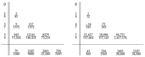
3.2.1. Method with Constant Coefficients

Chan and Tsai in [1] presented two 7th order methods with 5 stages. In this section we also consider methods with 5 stages, and follow the next procedure to derive a method of order 7.

• Using second simplifying assumption (6) we eliminate ${\widehat{a}}_{i,i-1}$ for $i=2,3,4,5$.
• Using third simplifying assumption (6) (except for the second component) we eliminate ${\widehat{a}}_{i,i-2}$ for $i=3,4,5$. We have to set ${\widehat{b}}_2=0$. Under this assumption the second condition for orders 5, 6 and 7 follow from the first condition.
• We solve the linear system equations

  $$\begin{array}{c}\hfill {\widehat{b}}^T{C}^{i}e=\frac{1}{(i+1)(i+2)},i=0,1,2,3\end{array}$$

  for the ${\widehat{b}}_i$ and derive

  $$\begin{array}{ccc}\hfill {\widehat{b}}_1& =& \frac{-3+c_4(5-10c_5)+5c_5+5c_3(1-2c_5+c_4(-2+6c_5))}{60c_3{c}_4{c}_5},\hfill \\ \hfill {\widehat{b}}_3& =& \frac{3-5c_5+5c_4(-1+2c_5)}{60c_3(c_3-c_4)(c_3-c_5)},{\widehat{b}}_4=\frac{3-5c_5+5c_3(-1+2c_5)}{60c_4(c_4+c_3)(c_4-c_5)},{\widehat{b}}_5=\frac{-3+c_3(5-10c_4)+5c_4}{60c_5(c_3-c_5)(c_5+c_4)}.\hfill \end{array}$$
• We solve the 3rd condition of order 6 for ${\widehat{a}}_{41}$.
• We solve the 3rd and 4th conditions of order 7 for ${\widehat{a}}_{51}$ and ${\widehat{a}}_{52}$.
• We solve ${\widehat{b}}^T{C}^{i}e=\frac{1}{(i+1)(i+2)}$ for $i=4,5$ and the last condition of order 7 for $c_3,c_4,c_5$.
• Finally we determine $c_2$ to minimize the next term of the amplification error
  $c_2=(5+3\sqrt{2})/28$

The stability function is

$$\begin{array}{c}\hfill R\left(z\right)=\sum _{k=0}^8\frac{z^k}{k!}+\frac{8+19\sqrt{2}}{\mathrm{9,948,960}}{z}^9+\frac{22+17\sqrt{2}}{\mathrm{79,591,680}}{z}^{10}\end{array}$$

the phase-lag and the dissipation are

$$\begin{array}{c}\hfill \varphi \left(v\right)=\frac{(425+228\sqrt{2})v^9}{\mathrm{119,387,520}}+O\left(v^{11}\right) \mathrm{and} \alpha \left(v\right)=\frac{(133+75\sqrt{2})v^{10}}{\mathrm{44,217,600}}+O\left(v^{12}\right)\end{array}$$

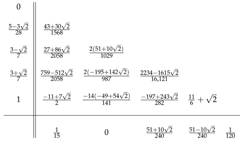
3.2.2. Method with Variable Coefficients

We also derive a phase-fitted and amplification-fitted method by modifying the first 7th order 5 stages method in [1]. Asking for $\varphi \left(v\right)=0$ and $\alpha \left(v\right)=0$ we modify the coefficients ${\widehat{b}}_1$ and ${\widehat{b}}_5$ as follows

$$\begin{array}{ccc}\hfill {\widehat{b}}_1& =& \frac{v^3\left(k_1+k_{2}cos\left(v\right)+k_{3}sin\left(v\right)\right)}{6720d}\hfill \\ \hfill {\widehat{b}}_5& =& \frac{91(v(5400-848v^2+35v^4)-5400sin\left(v\right))}{675d}\hfill \end{array}$$

where

$$\begin{array}{ccc}\hfill d& =& v^3\left(728-140v^2+15v^4\right)\hfill \\ \hfill k_1& =& (\mathrm{236,376}+\mathrm{21,812}{v}^2-\mathrm{13,985}{v}^4+800v^6)\hfill \\ \\ \hfill k_2& =& -6720v(728-140v^2+15v^4)\hfill \\ \hfill k_3& =& -960(-5096+2548v^2-245v^4+15v^6)\hfill \end{array}$$

The Taylor expansions of the coefficients ${\widehat{b}}_1$ and ${\widehat{b}}_5$ are

$$\begin{array}{ccc}\hfill {\widehat{b}}_1& =& \frac{71}{960}+\frac{v^6}{\mathrm{158,760}}-\frac{31v^8}{\mathrm{51,891,840}}-\frac{107v^{10}}{\mathrm{1,311,710,400}}-\frac{\mathrm{323,129}{v}^{12}}{\mathrm{48,343,086,792,000}}+\frac{\mathrm{29,534,363}{v}^{14}}{\mathrm{68,376,461,958,604,800}}+O\left(h^{16}\right)\hfill \\ \hfill {\widehat{b}}_5& =& \frac{13}{1350}-\frac{v^6}{\mathrm{362,880}}-\frac{131v^8}{\mathrm{259,459,200}}-\frac{2867v^{10}}{\mathrm{70,832,361,600}}+\frac{\mathrm{82,717}{v}^{12}}{\mathrm{1,570,995,456,000}}+\frac{\mathrm{7,318,085,461}{v}^{14}}{\mathrm{5,470,116,956,688,384,000}}+O\left(h^{16}\right)\hfill \end{array}$$

The order conditions now become

$$\begin{array}{cc}{\widehat{b}}^{T}e=\frac{1}{2}+\frac{v^6}{\mathrm{282,240}}+O\left(v^8\right)\hfill & {\widehat{b}}^T{C}^{5}e=\frac{1}{42}-\frac{v^6}{\mathrm{362,880}}+O\left(v^8\right)\hfill \\ {\widehat{b}}^{T}Ce=\frac{1}{6}-\frac{v^6}{\mathrm{362,880}}+O\left(v^8\right)\hfill & {\widehat{b}}^T{C}^2\widehat{A}Ce=\frac{1}{252}-\frac{v^6}{\mathrm{1,886,976}}+O\left(v^8\right)\hfill \\ {\widehat{b}}^T{C}^{2}e=\frac{1}{12}-\frac{v^6}{\mathrm{362,880}}+O\left(v^8\right)\hfill & {\widehat{b}}^{T}C\widehat{A}{C}^{2}e=\frac{1}{504}-\frac{v^6}{\mathrm{3,773,952}}+O\left(v^8\right)\hfill \\ {\widehat{b}}^T{C}^{3}e=\frac{1}{20}-\frac{v^6}{\mathrm{362,880}}+O\left(v^8\right)\hfill & {\widehat{b}}^T\widehat{A}{C}^{3}e=\frac{1}{840}-\frac{5v^6}{\mathrm{26,417,664}}+O\left(v^8\right)\hfill \\ {\widehat{b}}^T\widehat{A}Ce=\frac{1}{120}-\frac{v^6}{\mathrm{1,886,976}}+O\left(v^8\right)\hfill & {\widehat{b}}^T{\widehat{A}}^{2}Ce=\frac{1}{5040}-\frac{v^6}{\mathrm{17,611,776}}+O\left(v^8\right)\hfill \\ {\widehat{b}}^T{C}^{4}e=\frac{1}{30}-\frac{v^6}{\mathrm{362,880}}+O\left(v^8\right)\hfill & \\ {\widehat{b}}^{T}C\widehat{A}Ce=\frac{1}{180}-\frac{v^6}{\mathrm{1,886,976}}+O\left(v^8\right)\hfill & \\ {\widehat{b}}^T\widehat{A}{C}^{2}e=\frac{1}{360}-\frac{v^6}{\mathrm{3,773,952}}+O\left(v^8\right)\hfill \end{array}$$

We see that the modified method reduces to the original method as $v\to 0$.

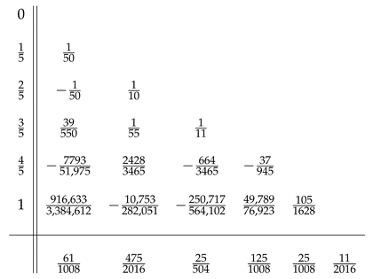
3.3. Methods with 6 Stages

As we have seen in the construction of the 7th order method using 5 stages there is only one free parameter $c_2$ which we determine by nullifying the next term of the amplification error. In order to have more flexibility for further optimization of the method we consider 6 stages. We impose the first two simplifying assumptions and follow the procedure:

• Using second simplifying assumption eliminate ${\widehat{a}}_{i,i-1}$ for $i=2,3,4,5,6$.
• Choose $c_2=0.2,c_3=0.4,c_4=0.6,c_5=0.8,c_6=1$.
• Solve the linear system equations

  $$\begin{array}{c}\hfill {\widehat{b}}^T{C}^{i}e=\frac{1}{(i+1)(i+2)},i=0,1,\dots ,5\end{array}$$

  for the ${\widehat{b}}_i$ for $i=1,\dots ,6$.
• Solve the remaining conditions for ${\widehat{a}}_{i,j}$, $i=3,4,5$, $j=1,\dots ,i-2$ and ${\widehat{a}}_{64}$.

The phase-lag order of this method is 8 and the dissipation order is 7. We find the remaining coefficients ${\widehat{a}}_{61}$, ${\widehat{a}}_{62}$, ${\widehat{a}}_{63}$ requiring the method to have phase-lag and dissipation order 12 and 9. The resulting method is:

The stability function is

$$\begin{array}{c}\hfill R\left(z\right)=\sum _{k=0}^9\frac{z^k}{k!}+\frac{z^{10}}{\mathrm{4,435,200}}+\frac{z^{11}}{\mathrm{39,916,800}}+\frac{z^{12}}{\mathrm{399,168,000}}\end{array}$$

the phase-lag and the dissipation are

$$\begin{array}{c}\hfill \varphi \left(v\right)=-\frac{191}{\mathrm{15,567,552,000}}{v}^{13}+O\left(v^{15}\right),\alpha \left(v\right)=-\frac{1}{\mathrm{19,958,400}}{v}^{10}+O\left(v^{14}\right).\end{array}$$

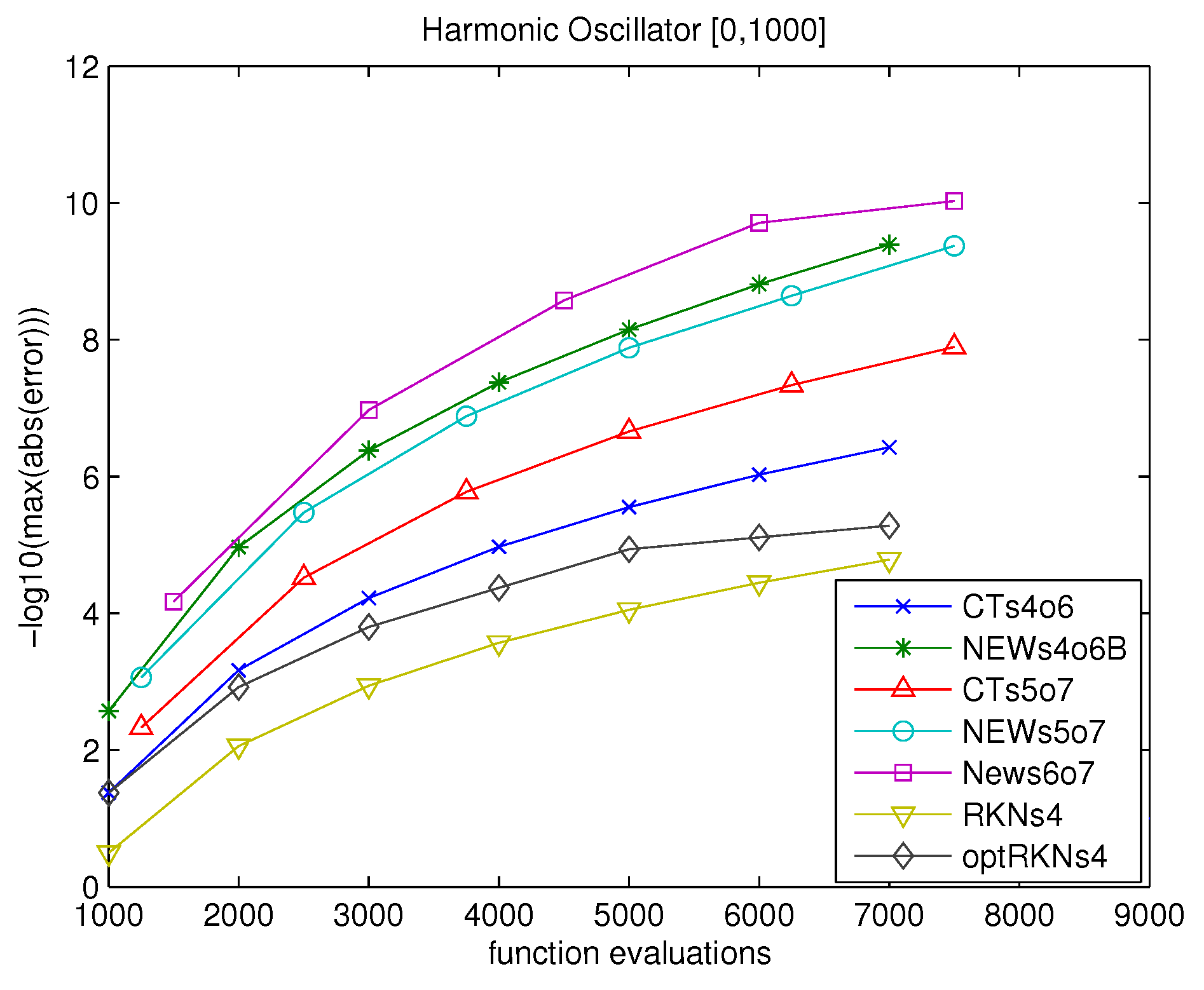
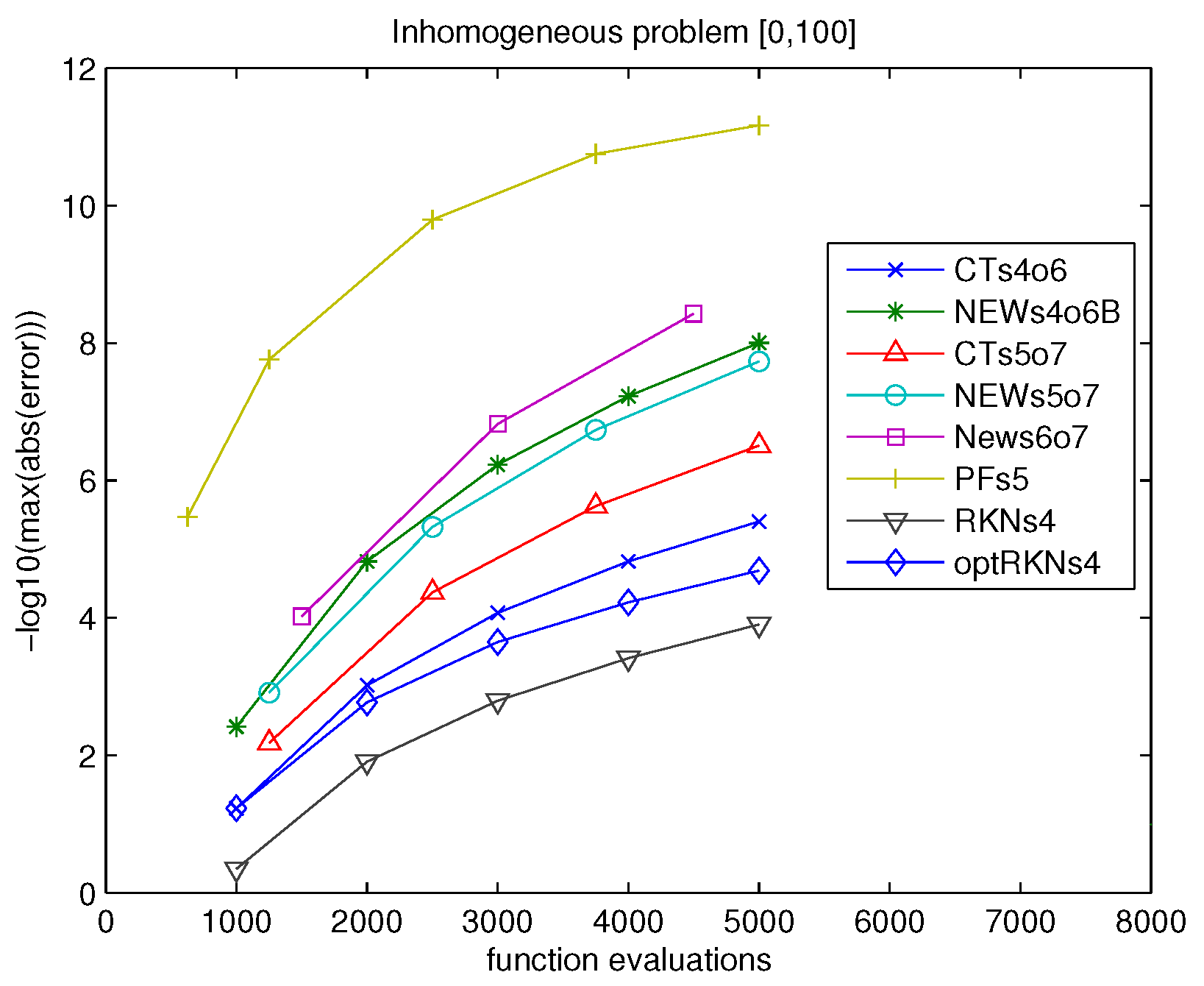
4. Numerical Results

The methods used to illustrate the efficiency of the new method are

• CTs4o6 the 6th order method with 4 stages in [1] (second method)
• CTs5o7 the 7th order method with 5 stages in [1] (first method)
• NEWs4o6B the new optimized 6th order method with 4 stages in Section 3.1 (second method)
• NEWs5o7 the new optimized 7th order method with 5 stages in Section 3.2.1
• NEWs6o7 the new optimized 7th order method with 6 stages in Section 3.3
• PFs5 the new phase-fitted and amplification-fitted method 5 stages in Section 3.2.2
• RKNs4 the 5th order Runge-Kutta-Nyström method with 4 stages ([33], p. 285)
• optRKNs4 the optimized Runge-Kutta-Nyström method with 4 stages, algebraic order 4 and phase-lag order 8 ([35]).

The problems used are

• The harmonic oscillator
• The inhomogeneous oscillatory problem that can be found in [36]
• The oscillatory linear system studied by Franco in [37]
• The almost periodic orbit problem studied by Stiefel and Bettis [38]

4.1. Problem 1

The harmonic oscillator

$$\begin{array}{ccc}\hfill y_1^{″}& =& -y_1,y_1\left(0\right)=1,y_1^{\prime }\left(0\right)=0\hfill \\ \hfill y_2^{\prime }& =& -y_2,y_2\left(0\right)=0,y_2^{\prime }\left(0\right)=1\hfill \end{array}$$

The exact solution is

$$\begin{array}{c}\hfill y_1\left(x\right)=cos\left(x\right)y_2\left(x\right)=sin\left(x\right).\end{array}$$

In Figure 1 we present the maximum absolute error of the solution in the interval $[0,1000]$. For this problem we use $w=1$. The fitted method has maximum absolute error less than ${10}^{-14}$ and for this reason it is not in the figure. The 3 methods with minimized phase-lag and amplification error have clearly superior performance compared with the methods in [1].

4.2. Problem 2

The inhomogeneous oscillatory problem

$$\begin{array}{c}\hfill y^{″}=-100y+99sin\left(x\right),y\left(0\right)=1,y^{\prime }\left(0\right)=11.\end{array}$$

The exact solution is $y\left(x\right)=cos\left(10x\right)+sin\left(10x\right)+sin\left(x\right)$. For this problem we use $w=10$. In Figure 2 we present the maximum absolute error of the solution in the interval $[0,100]$. Results again show the high accuracy of the fitted method, performance of all methods tested is similar to that for Problem 1.

4.3. Problem 3

The oscillatory linear system

$$\begin{array}{ccc}\hfill y_1^{″}+13y_1-12y_2& =& 9cos\left(2x\right)-12sin\left(2x\right),y_1\left(0\right)=1,y_1^{\prime }\left(0\right)=-4\hfill \\ \hfill y_2^{″}-12y_1+13y_2& =& -12cos\left(2x\right)+9sin\left(2x\right),y_2\left(0\right)=0,y_2^{\prime }\left(0\right)=8.\hfill \end{array}$$

The exact solution is

$$\begin{array}{ccc}\hfill y_1\left(x\right)& =& sin\left(x\right)-sin\left(5x\right)+cos\left(2x\right),\hfill \\ \hfill y_2\left(x\right)& =& sin\left(x\right)+sin\left(5x\right)+sin\left(2x\right).\hfill \end{array}$$

For this problem we use $w=5$. In Figure 3 we present the maximum absolute error of the solution in the interval $[0,100]$, we see that the new methods produce less absolute error.

4.4. Problem 4

The almost periodic orbit problem studied by Stiefel and Bettis [38]:

$$\begin{array}{ccc}\hfill y_1^{″}& =& -y_1+0.001cos\left(x\right),y_1\left(0\right)=1,y_1^{\prime }\left(0\right)=0\hfill \\ \hfill y_2^{″}& =& -y_2+0.001sin\left(x\right),y_2\left(0\right)=0,y_2^{\prime }\left(0\right)=0.9995\hfill \end{array}$$

The exact solution is

$$\begin{array}{c}\hfill y_1\left(x\right)=cos\left(x\right)+0.0005xsin\left(x\right),y_2\left(x\right)=sin\left(x\right)-0.0005xcos\left(x\right).\end{array}$$

For this problem we use $w=1$. In Figure 4 we present the maximum absolute error of the solution in the interval $[0,1000]$.

5. Conclusions

In this work two new methods are presented of order 7 with 5 and 6 stages and minimized dispersion and dissipation error, as well as a modified phase-fitted, amplification-fitted method with frequency dependent coefficients and 5 stages. The new methods have been tested on 4 oscillatory problems. The numerical results show that the new methods attain higher accuracy at the same cost.

References

1. Chan, R.P.K.; Tsai, A.Y.J. On explicit two-derivative Runge-Kutta methods. Numer. Alg. 2010, 53, 171–194. [Google Scholar] [CrossRef]
2. Kastlunger, K.H.; Wanner, G. Runge Kutta Processes with Multiple nodes. Computing 1972, 9, 9–24. [Google Scholar] [CrossRef]
3. Vigo-Aguiar, J.; Martín-Vaquero, J.; Ramos, H. Exponential fitting BDF–Runge–Kutta algorithms. Comput. Phys. Commun. 2018, 178, 15–34. [Google Scholar] [CrossRef]
4. Ramos, H.; Vigo-Aguiar, J. On the frequency choice in trigonometrically fitted methods. Appl. Math. Lett. 2010, 23, 1378–1381. [Google Scholar] [CrossRef] [Green Version]
5. Vigo-Aguiar, J.; Ramos, H. On the choice of the frequency in trigonometrically-fitted methods for periodic problems. J. Comput. Appl. Math. 2015, 277, 94–105. [Google Scholar] [CrossRef]
6. Ramos, H.; Kalogiratou, Z.; Monovasilis, T.; Simos, T.E. An optimized two-step hybrid block method for solving general second order initial-value problems. Numer. Algor. 2016, 72, 1089–1102. [Google Scholar] [CrossRef]
7. Simos, T.E.; Tsitouras, C. Explicit, ninth order, two step methods for solving inhomogeneous linear problems x(t) = Λx(t) + f(t). Appl. Numer. Math. 2020, 153, 344–351. [Google Scholar] [CrossRef]
8. Kovalnogov, V.N.; Simos, T.E.; Tsitouras, C. Ninth-order, explicit, two-step methods for second order inhomogeneous linear IVPs. Math. Meth. Appl. Sci. 2020, 43, 4918–4926. [Google Scholar] [CrossRef]
9. Alolyan, I.; Simos, T.E.; Tsitouras, C. Eighth-order, phase-fitted, four-step methods for solving y = f (x, y). Math. Meth. Appl. Sci. 2020, 43, 4016–4022. [Google Scholar] [CrossRef]
10. Hou, C.-C.; Simos, T.E.; Famelis, I.T. Neural network solution of pantograph type differential equations. Math. Meth. Appl. Sci. 2020, 43, 3369–3374. [Google Scholar] [CrossRef]
11. Medvedev, M.A.; Simos, T.E.; Tsitouras, C. Low-order, P-stable, two-step methods for use with lax accuracies. Math. Meth. Appl. Sci. 2019, 42, 6301–6314. [Google Scholar] [CrossRef]
12. Medvedeva, M.A.; Simos, T.E.; Tsitouras, C. Trigonometric fitted modification of RADAU5. Math. Meth. Appl. Sci. 2020, 43, 1582–1589. [Google Scholar] [CrossRef]
13. Lin, C.; Hsu, C.W.; Simos, T.E.; Tsitouras, C. Explicit, semi-symmetric, hybrid, six-step, eighth order methods for solving y = f (x, y). Appl. Comput. Math. 2019, 18, 296–304. [Google Scholar]
14. Medvedeva, M.A.; Simos, T.E.; Tsitouras, C. Variable step-size implementation of the sixth-order Numerov-type methods. Math. Meth. Appl. Sci. 2020, 43, 1204–1215. [Google Scholar] [CrossRef]
15. Alolyan, I.; Simos, T.E.; Tsitouras, C. Interpolants for sixth-order Numerov-type methods. Math. Meth. Appl. Sci. 2019, 42, 7349–7358. [Google Scholar] [CrossRef]
16. Medvedev, M.A.; Simos, T.E.; Tsitouras, C. Local interpolants for Numerov-type methods and their implementation in variable step schemes. Math. Meth. Appl. Sci. 2019, 42, 7047–7058. [Google Scholar] [CrossRef]
17. Fang, J.; Liu, C.; Simos, T.E.; Famelis, I.T. Neural network solution of single delay differential equations. Mediterr. J. Math. 2020, 17, 30. [Google Scholar] [CrossRef]
18. Liu, C.; Hsu, C.-W.; Simos, T.E.; Tsitouras, C. Phase-fitted, six-step methods for solving x = f (t, x). Math. Meth. Appl. Sci. 2019, 42, 3942–3949. [Google Scholar] [CrossRef]
19. Liu, C.; Hsu, C.-W.; Tsitouras, C.; Simos, T.E. Hybrid Numerov-type methods with coefficients trained to perform better on classical orbits. Bull. Malays. Math. Sci. Soc. 2019, 42, 2119–2134. [Google Scholar] [CrossRef]
20. Lin, C.; Chen, J.J.; Simos, T.E.; Tsitouras, C. Evolutionary derivation of sixth-order P-stable SDIRKN methods for the solution of PDEs with the method of lines. Mediterr. J. Math. 2019, 16, 69. [Google Scholar] [CrossRef]
21. Fang, J.; Liu, C.; Hsu, C.-W.; Simos, T.E.; Tsitouras, C. Explicit hybrid six-step, sixth order, fully symmetric methods for solving y = f (x, y). Math. Meth. Appl. Sci. 2019, 42, 3305–3314. [Google Scholar] [CrossRef]
22. Medvedev, M.A.; Simos, T.E.; Tsitouras, C. Hybrid, phase-fitted, four-step methods of seventh order for solving x (t) = f (t, x). Math. Meth. Appl. Sci. 2019, 42, 2025–2032. [Google Scholar] [CrossRef]
23. Medvedev, M.A.; Simos, T.E.; Tsitouras, C. Trigonometric-fitted hybrid four-step methods of sixth order for solving y (x) = f (x, y). Math. Meth. Appl. Sci. 2019, 42, 710–716. [Google Scholar] [CrossRef]
24. Fang, Y.; You, X.; Ming, Q. Trigonometrically fitted two-derivative Runge-Kutta methods for solving oscillatory differential equations. Numer. Algor. 2014, 65, 651–667. [Google Scholar] [CrossRef]
25. Monovasilis, T.; Kalogiratou, Z.; Simos, T.E. Trigonometrical fitting conditions for two derivative Runge Kutta methods. Numer. Algor. 2018, 79, 787–800. [Google Scholar] [CrossRef]
26. Kalogiratou, Z.; Monovasilis, T.; Simos, T.E. Construction of two derivative Runge Kutta methods of order five. AIP Conf. Proc. 2017, 1863, 560092. [Google Scholar]
27. Kalogiratou, Z.; Monovasilis, T.; Simos, T.E. New fifth-order two-derivative Runge-Kutta methods with constant and frequency-dependent coefficients. Math. Meth. Appl. Sci. 2019, 42, 1955–1966. [Google Scholar] [CrossRef]
28. Ahmad, N.A.; Senu, N.; Ismail, F. Phase-Fitted and Amplification-Fitted Higher Order Two-Derivative Runge-Kutta Method for the Numerical Solution of Orbital and Related Periodical IVPs. Math. Probl. Eng. 2017, 2017, 1871278. [Google Scholar] [CrossRef]
29. Fang, Y.; Zhang, Y.; Wang, P. Two-derivative Runge–Kutta methods with increased phase-lag and dissipation order for the Schrödinger equation. J. Math. Chem. 2018, 56, 1924–1934. [Google Scholar] [CrossRef]
30. Kalogiratou, Z.; Monovasilis, T.; Simos, T.E. Two-derivative Runge-Kutta methods with optimal phase properties. Math. Meth. Appl. Sci. 2020, 43, 1267–1277. [Google Scholar] [CrossRef]
31. Monovasilis, T.; Kalogiratou, Z.; Simos, T.E. Optimized two derivative Runge-Kutta methods for solving orbital and oscillatory problems. AIP Conf. Proc. 2019, 2116, 450107. [Google Scholar]
32. Butcher, J.C. The Numerical Analysis of Ordinary Differential Equations; John Wiley Sons: Hoboken, NJ, USA, 1987. [Google Scholar]
33. Hairer, E.; Norsett, S.; Wanner, G. Solving Ordinary Differential Equations I: Nonstiff Problems; Springer: Berlin/Heidelberg, Germany, 2002. [Google Scholar]
34. Houwen, P.J.V.; Sommeijer, B.P. Explicit Runge-Kutta (-Nyström) methods with reduced phase errors for computing oscillating solutions. SIAM J. Numer. 1987, 24, 595–617. [Google Scholar] [CrossRef] [Green Version]
35. Simos, T.E.; Dimas, E.; Sideridis, A.B. A Runge-Kutta-Nyström method for the numerical integration of special second-order periodic initial-value problems. J. Comput. Appl. Math. 1994, 51, 317–326. [Google Scholar] [CrossRef] [Green Version]
36. Vigo-Aguiar, J.; Ramos, H. Dissipative Chebyshev exponential-fitted methods for numerical solution of second-order differential equations. J. Comput. Appl. Math. 2003, 158, 187–211. [Google Scholar] [CrossRef] [Green Version]
37. Franco, J.M. A class of explicit two-step hybrid methods for second-order IVPs. J. Comput. Appl. Math. 2006, 187, 41–57. [Google Scholar] [CrossRef] [Green Version]
38. Stiefel, E.; Bettis, D.G. Stabilization of Cowell’s method. Numer. Math. 1969, 13, 154–175. [Google Scholar] [CrossRef]
Figure 1. Problem 1 (Harmonic Oscillator) [0, 1000].
Mathematics 09 00232 g001
Figure 2. Problem 2 (Inhomogeneous Oscillatory Problem) [0, 100].
Mathematics 09 00232 g002
Figure 3. Problem 3 (Oscillatory Linear System) [0, 100].
Mathematics 09 00232 g003
Figure 4. Problem 4 (Stiefel-Bettis) [0, 1000].
Mathematics 09 00232 g004
Publisher’s Note: MDPI stays neutral with regard to jurisdictional claims in published maps and institutional affiliations.