MP-CE Method for Space-Filling Design in Constrained Space with Multiple Types of Factors

Abstract

Space-filling design selects points uniformly in the experimental space, bringing considerable flexibility to the complex-model-based and model-free data analysis. At present, space-filling designs mostly focus on regular spaces and continuous factors, with a lack of studies into the discrete factors and the constraints among factors. Most of the existing experimental design methods for qualitative factors are not applicable for discrete factors, since they ignore the potential order or spatial distance between discrete factors. This paper proposes a space-filling method, called maximum projection coordinate-exchange (MP-CE), taking into account both the diversity of factor types and the complexity of factor constraints. Specifically, the maximum projection criterion and distance criterion are introduced to capture the “bad” coordinates, and the coordinate-exchange and the optimization of experimental design are realized by solving one-dimensional constrained optimization problem. Meanwhile, by adding iterative perturbations to the traditional coordinate exchange process, the adjacent areas of the local optimal solution are explored and the optimum performances of the current optimal solution are retained, while the shortcomings of random restart are effectively avoided. Experiments in the regular space and constraint space, as well as experimental design for the terminal interception effectiveness of a missile defense system, show that the MP-CE method significantly outperforms existing popular space-filling design methods in terms of space-projection properties, while yielding comparable or superior space-filling properties.

1. Introduction

The experimental design aims to strategically select a combination of experimental factors, so as to maximize benefits at the minimum computational cost. Space-filling designs are used to observe the response by placing a set of experimental points uniformly in the design space, which can provide insight into the performance of the experimental object in the whole experimental space and has high flexibility in exploring the relationship between the factors and the response. Typical space-filling design methods include Latin hypercube design (LHD) and uniform design. LHD is the standard method for uniformly placing points on each univariate dimension [1]. Johnson, Moore, and Ylvisaker proposed a method to optimize LHD using space-filling criterion, including the Maximin LHD (MmLHD) that maximizes the minimum distance between two points, and the Minimax LHD that minimizes the maximum distance between two points [2]. Kaitai Fang and Yuan Wang put forward a uniform design to find the test points uniformly distributed in the design space [3]. Joseph believes that the computer experiment output is deterministic, and any repeated design points will lead to a waste of computing resources. Therefore, a good design of computer experiment should be non-overlapping. LHD improves one-dimensional projection properties but cannot guarantee good space-filling properties in higher-dimensional subspaces. Therefore, Joseph, Gul and Ba et al. proposed the maximum projection (MaxPro) design, which can simultaneously optimize the space-filling properties of the design points with respect to all possible subsets of factors [4]. The test proves that it also has a good performance in the space-filling distance.

The current experimental design mainly focuses on the continuous numerical factors in the regular space, however, the actual experiments may involve discrete numerical factors and ordered qualitative factors, and there may be complex constraints between factors. For example, in the flight experiment of ship-to-air missile, the experimental factors include target speed, target height, target distance and so on. The target speed is generally a discrete numerical factor corresponding to the specific type of target, for example, the speed of a helicopter in a low-speed hovering state can be regarded as 0 m/s, while that of a subsonic anti-ship missile is around 300 m/s. The target height has three levels of high, medium, and low altitude, and the target distance has three levels of near, medium and far. They are both qualitative factors and their levels are in order. Furthermore, there are constraints between the target speed and the target height.

In a bid to solve the above problems of experimental design with discrete factors and qualitative factors, this paper proposes a coordinate exchange algorithm based on MaxPro criterion and distance criterion, namely the MP-CE method, which incorporates discrete factors for optimization, and calculates the probability of coordinate exchange based on distance properties and projection properties to avoid falling into a local optimal solution prematurely. Each time the local optimal solution is found, iterated perturbations are added to avoid the shortcomings of random restart of the coordinate exchange algorithm. As ordered qualitative factors can be transformed into discrete numerical factors, discrete numerical factors and ordered qualitative factors are collectively referred to as discrete factors in the following description.

2. Literature Review

2.1. Experimental Design with Discrete Factors

The space-filling designs with qualitative factors include the slice Latin hypercube design [5,6,7], the marginally coupled design [8,9], the clustering filling design and so on [10,11]. The optimal design strategy for experiments with discrete factors differs from that for experiments with continuous factors, as the level of discrete factors may be repeated, and it also differs from that for experiments with qualitative factors, because the difference between qualitative factors cannot be measured by distance. However, the current main strategy for experimental designs with discrete factors is to ignore the order between factors and treat them as disordered qualitative factors. Another strategy is to treat the discrete numerical factors as continuous factors and then round each of them to the nearest discrete value. The problem with this method is that the final design may not be optimal, or even worse than the local optimal solution. Joseph first extends its MaxPro design for experiments with continuous, discrete, and qualitative factors, which can achieve good space-filling properties in the whole design space and all possible sub dimensional projections [12]. The design matrix is randomly initialized by generating a random LHD and folding each value of the factors to the closest given discrete level. and the simulated annealing algorithm is used to iteratively search the optimal solution by randomly exchanging two coordinates in a column of the design matrix. In fact, this method does not change the distribution of discrete levels in the initial design, thus it is not suitable for experiments with constraints between factors.

2.2. Experimental Design in Constrained Space

The typical methods of constructing space-filling designs in hypercubes are usually not suitable for constrained experimental spaces. Although it is possible to create design in unconstrained space and remove unacceptable points, this may result in unexplored areas of the design space and require additional work to ensure that the number of design points matches the requirements of the experiment. Draguic, Santner, and Dean introduced the CoNcaD algorithm [13], which is used for a space-filling design in bounded non-rectangular regions, focusing on maximum and low-dimensional properties. Beal et al. (2014) improved the WSP algorithm to construct a space-filling design, which can be applied to experimental designs with specific constraints and can increase the observation density of specific regions of interest [14]. Lulu Kang (2019) provided a random coordinate exchange algorithm for constructing experimental designs with space-filling criterion in arbitrary regular or irregular constrained spaces, which improves the optimization efficiency of coordinate exchange [15]. Lekivetz and Jones (2015) proposed a fast flexible space-filling (FFF) design [16], which clusters random points in the design space to generate design. Subsequently, the FFF algorithm was extended to allow qualitative factors to be added to the design, while maintaining the flexibility of quickly creating space-filling designs in rectangular and non-rectangular spaces [10]. However, none of these methods propose an appropriate measure of space-filling properties for designs with discrete factors.

3. The MP-CE Method

Assuming there are p₁ continuous factors, namely X₁,…,X_p1, and p₂ discrete factors, namely X_p1+1,…,X_p, and p₁ + p₂ = p. The number of the discrete levels of the l-th discrete factor X_l(l = p₁ + 1,…,p), is denoted as $m_l$. There are s constraints between factors, denoted by the vector cons = (constraint₁,…,constraint_s), then the value space of factors can be denoted as $\underset{cons}{R^p}$. Our task is to construct a design matrix D_n×p of the input factors, where the i-th row x_i = (x_i1, x_i2,…,x_ip) represents the i-th design point, so that these n design points representing n experiments are uniformly filled in the design space.

In the literature [17,18,19,20] it was found that the ideal space-filling design should possess high separation distance, low fill distance and excellent projection distance. The separation distance refers to the minimum distance between any two experimental points. Designs with high separation distance aim to maximize the following criterion:

$$\underset{x_i,x_j\in D}{\min }d(x_i,x_j)$$

(1)

The fill distance refers to the maximum distance between a given position in the design space and the nearest test point. Designs with low filling distance aim to minimize the following criterion:

$$\underset{x\in {\underset{cons}{R}}^p}{\max }\underset{x_i\in D}{\min }d(x,x_i)$$

(2)

There is almost no contradiction between the above two distance criteria. For projection distance, the MaxPro design with multiple factors proposed by Joseph can achieve good projection properties in the whole design space and all possible sub dimensional spaces. Referring to the literature [12], this method minimizes the following criterion:

$$\mathrm{MaxPro}(D)={\left\{\frac{1}{\left(\begin{array}{c}n\\ 2\end{array}\right)}{\displaystyle \sum _{i=1}^{n-1}{\displaystyle \sum _{j=i+1}^n\frac{1}{{\displaystyle \prod _{l=1}^{p_1}{\left(x_{il}-x_{jl}\right)}^2}{\displaystyle \prod _{k=1}^{p_2}{\left(\left|x_{ik}-x_{jk}\right|+\frac{1}{m_k}\right)}^2}}}}\right\}}^{\frac{1}{p_1+p_2}}$$

(3)

Expanding the above ideas, this paper proposes a new space-filling design method, namely MP-CE, which applies the MaxPro criterion and distance criterion to guide coordinate exchange, making it suitable for experimental designs with discrete factors and constraints between factors.

MP-CE selects a “bed” coordinate of the current design by applying the coordinate selection criterion, exchanges it into a better coordinate to improve the current design criterion to generate a new design, which reduces the high-dimensional optimization problem to one-dimensional optimization, and it overcomes the problem that the algorithm is easy to fall into local optimization by applying iterated perturbation, as shown in Figure 1. Next, we will describe coordinate selection, coordinate exchange and iterated perturbation.

3.1. Coordinate Selection

The coordinates to be exchanged, also known as ‘bad’ coordinates, are selected according to the projection criterion and distance criterion. Define the projection coefficient of the l-th dimension between two points x_i and x_j as:

$$pro(x_{il},x_{jl})=\frac{1}{\left|x_{il}-x_{jl}\right|+\omega },\omega =\{\begin{array}{c}0,l=1,\cdots ,p_1\\ \frac{1}{m_l},l=p_1+1,\cdots ,p\end{array}$$

(4)

The steps of selecting coordinates are as follows:

(1) From the row vector of the design matrix, [x₁, x₂,…, x_n]^T, a pair of “bad” design points (x_a, x_b) are randomly selected with a probability proportional to the following formula:

$$\frac{{\displaystyle \prod _{l=1}^p{\left(pro(x_{il},x_{jl})\right)}^2}}{{\displaystyle \sum _{i=1}^{n-1}{\displaystyle \sum _{j=i+1}^n{\displaystyle \prod _{l=1}^p{\left(pro(x_{il},x_{jl})\right)}^2}}}}$$

(5)

From the perspective of numerical stability, when p is large, the following formula can be used instead:

$$\frac{{\left({\displaystyle \prod _{l=1}^{p}pro(x_{il},x_{jl})}\right)}^{-p}}{{\displaystyle \sum _{i=1}^{n-1}{\displaystyle \sum _{j=i+1}^n{\left({\displaystyle \prod _{l=1}^{p}pro(x_{il},x_{jl})}\right)}^{-p}}}}$$

(6)

(2) Calculate the sum of the projection coefficients of x_a, x_b and other design points respectively, and determine the row coordinate index i (i = a or i = b) with a probability proportional to the following formula:

$$\left(\frac{{\displaystyle \sum _{r\ne a,r\ne b}^{n}pro(x_a,x_r)}}{{\displaystyle \sum _{r\ne a,r\ne b}^{n}pro(x_a,x_r)}+{\displaystyle \sum _{r\ne b,r\ne a}^{n}pro(x_b,x_r)}},\frac{{\displaystyle \sum _{r\ne b,r\ne a}^{n}pro(x_b,x_r)}}{{\displaystyle \sum _{r\ne a,r\ne b}^{n}pro(x_a,x_r)}+{\displaystyle \sum _{r\ne b,r\ne a}^{n}pro(x_b,x_r)}}\right)$$

(7)

(3) Finally, in the pair of “bad” design points (x_a, x_b), the column coordinate index j (j = 1,…,p) is determined with a probability proportional to the following formula:

$$\frac{pro(x_{al},x_{bl})}{{\displaystyle \sum _{l=1}^{p}pro(x_{al},x_{bl})}}$$

(8)

3.2. Coordinate Exchange

According to the above steps, the coordinate to be improved is selected, which is x_ij, and it will be optimized next. First of all, keep the remaining coordinates x_il(l ≠ j) unchanged, which belongs to point x_i, and substitute the values of the remaining coordinates into the set of constraints cons = (constraint₁,…,constraint_s), then solve the constraint problem for x_ij, and get the updated range of x_ij, which is denoted as $\left[lo{w}_{x_{ij}},u{p}_{x_{ij}}\right]$. Solve the one-dimensional optimization problem in the new range and use the obtained optimal solution x_ij* to generate new design D* iteratively.

For each iteration to solve the one-dimensional optimization problem, the sum of the projection coefficients between other points remains unchanged except for the projection coefficients involved in point x_i. The sum of the projection coefficients between the other points is expressed by the following formula.

$${\displaystyle \sum _{k=1,k\ne i}^{n-1}{\displaystyle \sum _{f=k+1,f\ne i}^n{\displaystyle \prod _{l=1}^p{\left(pro(x_{kl},x_{fl})\right)}^2}}}$$

(9)

The projection coefficients between point x_i and other points remain unchanged except the j-th dimension, and the projection coefficients matrix is expressed as follows:

$${\left[{\left(\underset{f\ne i,l=1,l\ne j}{pro}(x_{il},x_{fl})\right)}^2,\cdots ,{\left(\underset{f\ne i,l=p,l\ne j}{pro}(x_{il},x_{fl})\right)}^2\right]}_{(n-1)\times (p-1)}$$

(10)

where the column vector ${\left(\underset{f\ne i,l\ne j}{pro}(x_{il},x_{fl})\right)}^2$ is expressed as

$${\left[{\left(\underset{f=1,f\ne i,l\ne j}{pro}(x_{il},x_{fl})\right)}^2,\cdots ,{\left(\underset{f=n,f\ne i,l\ne j}{pro}(x_{il},x_{fl})\right)}^2\right]}^{\mathrm{T}}$$

when the coordinate x_ij is updated, the projection coefficients between point x_i and other points in the j-th dimension will all be updated accordingly, which can be represented by the following column vector:

$${\left[{\left(\underset{f=1,f\ne i}{pro}(x_{ij},x_{fj})\right)}^2,\cdots ,{\left(\underset{f=n,f\ne i}{pro}(x_{ij},x_{fj})\right)}^2\right]}^{\mathrm{T}}$$

(11)

After Formulas (10) and (11) are combined, the sum of the projection coefficients between point x_i and other points is calculated, and it is updated as follows:

$${\displaystyle \sum _{f=1,f\ne i}^n{\displaystyle \prod _{l=1}^p{\left(pro(x_{il},x_{fl})\right)}^2}}$$

(12)

According to Formula (3), combining Formulas (9) and (12), our objective function is to minimize Formula (13):

$${\left\{\frac{2\left({\displaystyle \sum _{k=1,k\ne i}^{n-1}{\displaystyle \sum _{f=k+1,f\ne i}^n{\displaystyle \prod _{l=1}^p{\left(pro(x_{kl},x_{fl})\right)}^2}}}+{\displaystyle \sum _{f=1,f\ne i}^n{\displaystyle \prod _{l=1}^p{\left(pro(x_{il},x_{fl})\right)}^2}}\right)}{n(n-1)}\right\}}^{\frac{1}{p}}$$

(13)

To simplify the calculation, the one-dimensional optimization problem of coordinate exchange can be simplified as follows:

$$x_{ij}^{*}\leftarrow \underset{x_{ij}\in \left[lo{w}_{x_{ij}},u{p}_{x_{ij}}\right]}{\arg \min }{\displaystyle \sum _{f=1,f\ne i}^n{\displaystyle \prod _{l=1}^p{\left(pro(x_{il},x_{fl})\right)}^2}}$$

(14)

For the implementation of our method, formula (14) is calculated using the R package ‘nloptr’ (Ypma, 2020). The entire coordinate exchange algorithm repeats the coordinate-exchange optimization and compares the projection properties according to formula (13). If the new design matrix D* obtained after the coordinate exchange is better than the current optimal design matrix D, the coordinate exchange is implemented, and the current optimal design is updated. Algorithm 1 summarizes the detailed steps of coordinate exchange.

Algorithm 1 MaxPro coordinate-exchange.

Input: n:size of the design p1:number of continuous factors p:number of factors cons:constraint functions bounds:bounds of continuous factors and sets of discrete factors.

D ← randomly generate an initial matrix with consandbounds as inputs

fori = 1,…,n − 1 for j = i + 1,…,n

for l = 1,…,p

pro(xil,xjl) ← use Equation (4)

End for

End for

End for

opt ← use Equation (3)

i.pair ← sampl a pair of “bed” points with Equation (6) as the probability

i ← sampl the “bed” point with Equation (7) as the probability

j ← sampl the “bed” coordinate with Equation (8) as the probability

[lowxij,upxij] ← generate new bound with cons,boundsand xil(l ≠ j) as inputs

if j = 1,…,p1

xij* ← use nloptr with Equation (14) and [lowxij,upxij] as input

else xij* ← use Equation (14) and [lowxij,upxij]

pro(xil,xjl)* ← use Equation (12)

opt(D*) ← use Equation (13)

if opt(D*) < opt

opt ← opt(D*)

xij ← xij*

D ← D*

Output: D:design matrix opt:objective function value.

3.3. Iterated Perturbation

The local search optimization algorithm may be affected by the initial design to a certain extent. Generally, the problem of easily falling into local optimal solution is overcome by repeating the search (i.e., restarting the search with a new set of initial experimental points). Studies have found that the restart strategy merely expands the scope of search and increases the chance of avoiding local optimal solution. In addition, the strategy lacks stability and is not applicable to large-scale experimental designs [21,22]. Therefore, we add iterated perturbation to MP-CE, and set the perturbation operator as the coordinate. The iterated perturbation strategy is shown in Figure 1. Given the current optimal solution D, it is perturbed to jump out of the local area, and the perturbed solution is denoted as D’. Then the MP-CE algorithm is applied to D’, and a new current optimal solution is obtained. The local search and perturbation are carried out repeatedly to return to the optimal design after the number of iterations is reached.

Through experimental research, Cuervo found that the size of the perturbation operator that leads to the best algorithm performance is PERT_SIZE = 10% [23]. Drawing reference from its experimental conclusion, this paper sets the scale of coordinate perturbation to 10% × (n × p). Algorithm 2 shows the detailed steps of iterated perturbation.

Algorithm 2 Iterated perturbation.

Input: maxstep:number of iterations. D:use Algorithm 1; opt:use Algorithm 1;

step ← 0

while step < maxstep

step ← step + 1

D’ ← D

repeat

i ← randomly sample from 1 to n

j ← randomly sample from 1 to p

[lowxij,upxij] ← generate new bound with cons,boundsand xil(l ≠ j)

xij ← randomly generate in [lowxij,upxij]

until 10% × (n × p) coordinates are perturbed break

update D’

D’* ← use Algorithm 1

opt(D’*) ← use Equation (13)

if opt(D’*) < opt

D ← D’*

opt ← opt(D’*)

end while

Output: D:design matrix opt:objective function value.

4. Experimental Setup

4.1. Comparison Method

We chose several popular space-filling experimental design methods for comparison. The following is a brief introduction to these comparison methods.

(1) uniform design

Kaitai Fang and Yuan Wang jointly put forward the uniform design in 1978, using the uniform distribution theory in number theory to select n experimental points, and applying number theory to ensure the points were uniformly distributed within the integration range, and ensure the distribution points were sufficiently close to various values of the integrand function. The uniform design is obtained through the “space-filling: uniform design” in the DOE of JMP software.

(2) MmLHD

In the LHD, each factor has as many levels as designed, and these levels are uniformly spaced from the lower limit to the upper limit of the factor. The MmLHD optimizes LHD by maximizing the minimum distance between design points. The MmLHD is obtained through the maximinLHS function in R packet “lhs” (Carnell, 2020).

(3) Fast flexible space-filling (FFF)

The FFF design (Lekivetz and Jones, 2015) [16], which is a space-filling design based on the Fast Ward clustering algorithm. First obtain a large sample $U\left(\chi \right)$, then use the Ward’s minimum variance criterion (Ward Jr, 1963) for systematic clustering to form n clusters, and finally obtain the final design points by using the MaxPro optimality criterion. The FFF design is obtained through “space-filling: FFF Design: MaxPro criterion “in the DOE of JMP software.

(4) Maximum projection

The maximum projection designs with quantitative and qualitative factors (MaxProQQ), which is a maximum projection design with quantitative and qualitative factors. First, the design matrix is randomly initialized by generating a random LHD and folding n levels to the nearest given discrete values of the factor. Use the simulated annealing algorithm (Morris and Mitchell 1995) and MaxPro criterion to optimize the initial design, and iteratively optimize in the design space by randomly selecting two coordinates in a column in the design matrix to exchange. The MaxProQQ design is obtained through the MaxProQQ function in R packet “MaxPro” (Ba, 2018).

4.2. Implementation Details

To implement the MP-CE method, we set the number of internal loop searches to 100 and the number of external perturbations to 20. We used the continuous optimization algorithm nloptr to optimize the design matrix to find the local optimal solution of coordinate-exchange. This function can be obtained in the R package “nloptr”. The scale of the coordinate perturbation is set to 10% × (n × p).

For the initial design matrix, the continuous factors are uniformly distributed using the LHD, and the discrete factor levels are allocated to each design point by random sampling, and the feasibility of each design point is tested according to the constraints. The comparison experiments, MmLHD and MaxProQQ, adopt the same initial design as MP-CE. The number of iterations of MmLHD and MaxProQQ is set to 1000. The number of restarts for uniform design and FFF design is set to 20.

In Section 3, we have pointed out the properties that the ideal space-filling design should have, so in the experimental analysis of this paper, we use the MaxPro index to evaluate the space projection of the design, see formula (3), and use the index ${\varphi }_p$ based on distance to evaluate the space-filling. The ${\varnothing }_p$ is defined as follows:

$${\varphi }_p(D)={({\displaystyle \sum _{i=1,i>j}^n{d}_{ij}^{-p}})}^{\raisebox{1ex}{$1$}\!\left/ \!\raisebox{-1ex}{$p$}\right.}$$

(15)

where p is a positive integer and d_ij represents the distance between any two design points in the design matrix D_n×m, that is, the row vectors x_i and x_j.

5. Results and Analysis

5.1. Space-Filling Design in [0,1]^p

In this section, we compare the uniform design, MmLHD, FFF design, MaxProQQ design, and our MP-CE design. We conducted experiments on several different input configurations, including p = 2, p = 6, p = 10, and n = 25, n = 50, n = 100. The experiments on these input configurations led to basically similar conclusions.

Table 1. Performance comparison of space-filling design methods.

	${\mathit{\varphi }}_{\mathit{p}}$			MaxPro
	p = 2	p = 6	p = 10	p = 2	p = 6	p = 10
Uniform	81.44828	47.21208	33.47989	111.3468	39.33209	28.76458
MmLHD	119.7706	77.44039	69.75027	118.8044	39.82723	29.03003
FFF	63.1522	35.96823	31.62291	102.3185	36.18002	25.88254
MaxProQQ	63.58684	39.34273	29.84868	113.1384	36.84071	25.44766
MP-CE	63.28473	34.13822	28.93871	100.8138	34.56103	24.36288

takes n = 50 as an example to list the performance of different experimental design methods in 2, 6 and 10-dimensional space. The results produced by the best performer and the best baseline in each column are boldfaced and underlined, respectively.

First of all, it can be seen that MP-CE outperforms other space-filling design methods, i.e., uniform design, MmLHD, FFF and MaxProQQ in terms of ${\varphi }_p$ and MaxPro. When the dimension of the experimental space changes from 2 to 10, the improvements of MP-CE over the best baseline are increased. In detail, the improvements are −0.21%, 5.09%, and 3.05% in terms of ${\varphi }_p$, 1.47%, 4.47% and 4.26% in terms of MaxPro when p = 2, p = 6, p = 10, respectively. It shows the superiority of this method in the space-filling of high-dimensional. Since MP-CE is designed based on the MaxPro criterion, the improvements of MP-CE in terms of MaxPro are larger than that of ${\varphi }_p$. In addition, both MaxProQQ and MP-CE start with the same initial design, and MP-CE outperforms MaxProQQ in terms of ${\varphi }_p$ and MaxPro, indicating that the perturbed coordinate–exchange algorithm also has certain advantages compared with the simulated annealing algorithm. The initial design also has a certain impact on the final effect of MP-CE, especially when the number of design points is small or the dimension is low, it can be overcome by increasing the number of iterations.

5.2. Space-Filling Design in Constrained Spaces

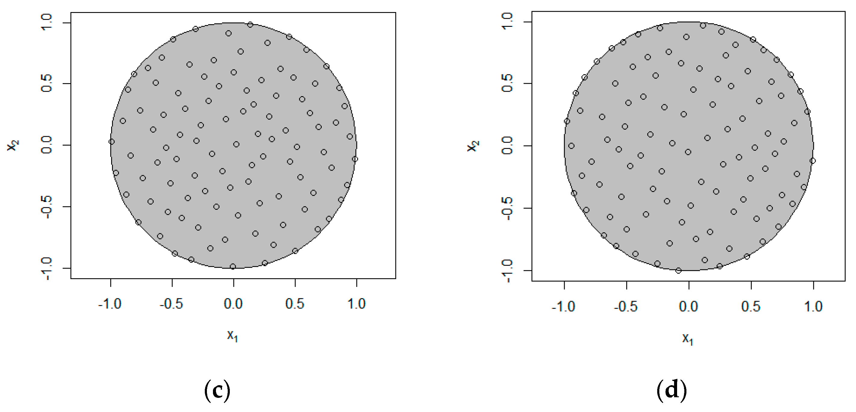
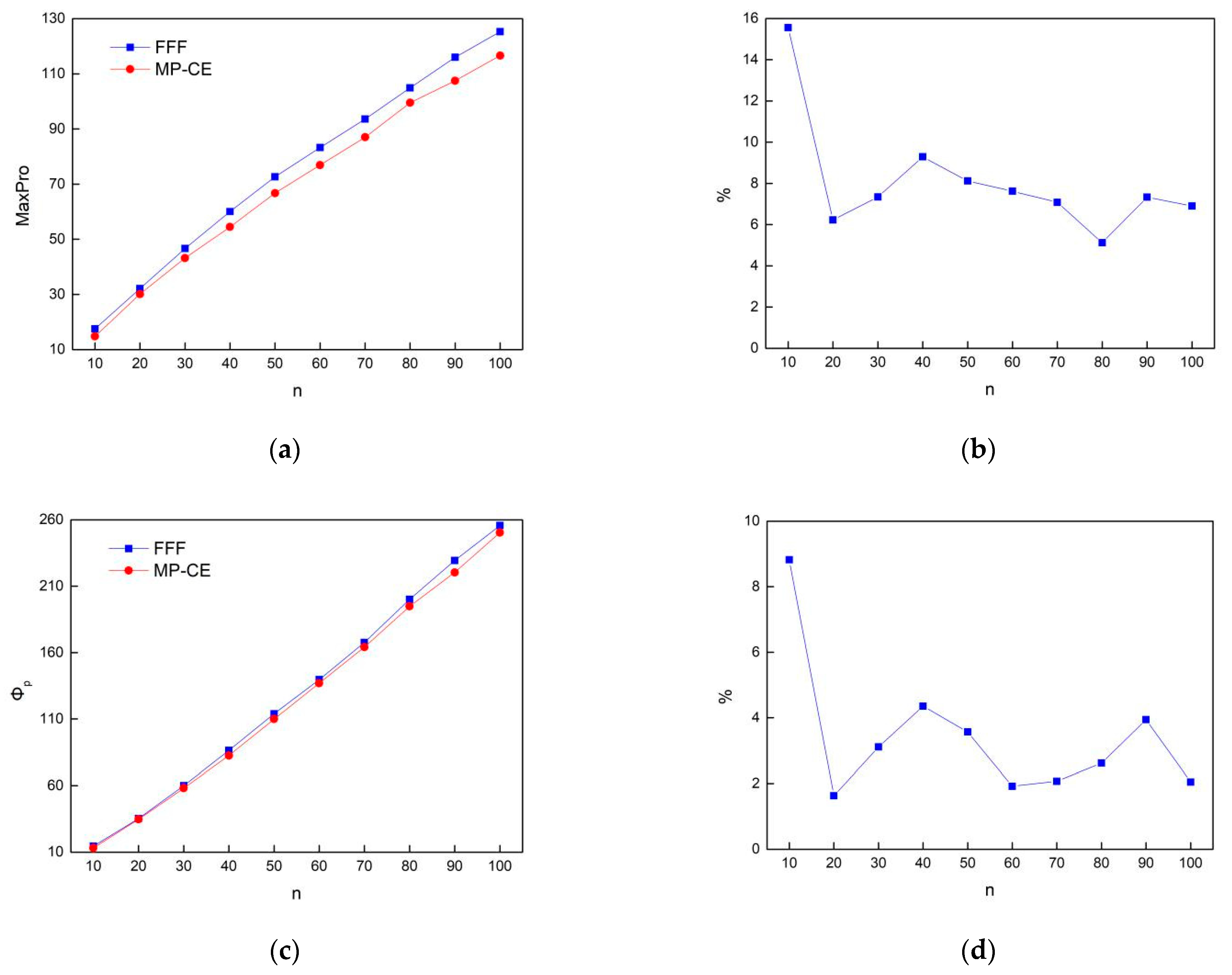
This section will discuss the performance of the MP-CE design in constrained spaces. The experimental setting is the same as above, considering a constrained space of p = 2, Figure 2 plots the design results of n = 10 and n = 100. FFF, which performs well in the regular space and is used for comparison with MP-CE. Figure 3 compares these two methods in terms of the space projection and space-filling properties with different run sizes. As the measurements are different with different run sizes, Figure 3b,d show the performance improvement of MP-CE over FFF in terms of ratio, in a bid to make the results more intuitive. The following two points can be observed from Figure 2 and Figure 3. On the one hand, in the constrained space of p = 2, FFF and MP-CE have very close performance in terms of space-filling and space-projection, which confirms the applicability of our method in constrained spaces. On the other hand, compared with FFF, MP-CE provides optimal maximin and maximum projection design for each run size. In particular, MP-CE performs better as the size of the design increases.

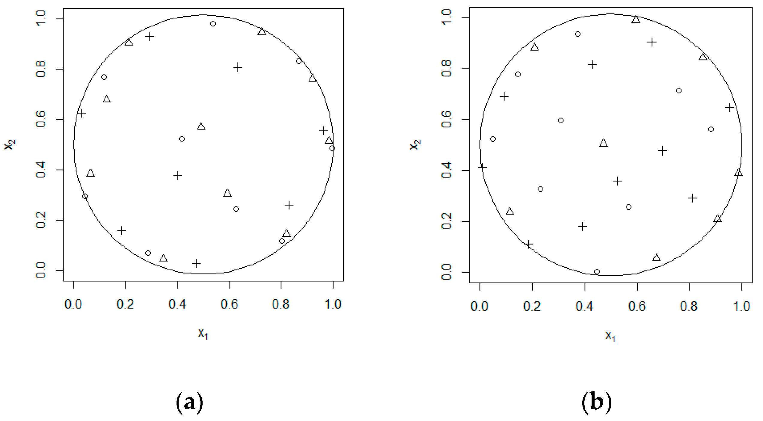
For the above experimental design in a 2-dimensional constrained space, a discrete factor was added, with the value of 0, 0.5, 1, and the constraints between the factors remain unchanged.

For the purpose of comparing with MP-CE method, we adopted the “custom designs” platform of JMP, which can define factor types and factor constraints. Enter two continuous factors, specify constraints on the design space, and impose constraints on the third factor to make it infinitely approximate to the level of discrete value. Then select the FFF design and set the optimality criterion to MaxPro. Set n = 27. In Figure 4, we made the 2-dimensional mapping discrete diagram to show the results from the two experimental design methods. The circle, triangle, and plus sign in the Figure represent x₃ = 0, 0.5, 1, respectively. It can be seen from the diagram that the space-filling performance of the FFF is obviously inferior to that of MP-CE.

5.3. Case Study

Section 5.1 and Section 5.2 discussed the performance of MP-CE in rule space and constraint space. This section will discuss the applicability and performance of MP-CE in the constrained space with multiple types of factors, in combination with an experimental design for the terminal interception effectiveness of the missile defence system.

At the terminal of the missile-target intersection, when the missile attacks the target, the kill probability is associated with many factors, including the accuracy of the missile guidance system, the miss distance, the positional relationship when the missile and target meet, the initiation trigger performance of the warhead, the explosion power, and the anti-damage ability of the target, etc. In one word, it is the result of randomly combined multiple factors.

Table 2. Experimental actors.

Type	Factor	Levels
continuous factor	encounter distance	5–50 (km)
discrete factor	target speed	0, 250, 300, 800, 1000 (m/s)
	target height	ultra-low altitude, hollow altitude, high altitude
	target maneuver overload	4, 5, 6, 7, 8, 9(G)

lists the factors that may be related to missile interception effectiveness. The assessment of missile intercepting low-speed hovering helicopter targets, subsonic aircraft targets, subsonic missile targets, supersonic maneuverable missile targets, and supersonic anti-ship missile targets correspond to the following target speeds in Table 2. Regarding the constraint between the factors, when the target speed is 0, the target height can only correspond to ultra-low altitude and hollow altitude.

First of all, the experimental factors are normalized. The encounter distance is mapped to X₁ = [0,1], the target speed is converted to discrete values X₂ = 0, 0.25, 0.3, 0.8, 1, the target height is converted to discrete values X₃ = 0, 0.7, 1, and the target maneuver overload is converted to discrete values X₄ = 0, 0.2, 0.4, 0.6, 0.8, 1. Constraint between factors is when X₂ = 0, X₃ = 0 or 0.7.

Additionally, we used the FFF design of JMP as the baseline, set the optimality criterion to MaxPro, entered 4 continuous factors, and imposed constraints on the second, third, and fourth factors to make it infinitely approximate the value of each discrete level. Taking n = 10 as an example, the final experimental design results returned by FFF and MP-CE are shown in

Table 3. Comparison of design results.

	FFF				MP-CE
factor	X1	X2	X3	X4	X1	X2	X3	X4
Scheme	0.57758	1	0.7	1	0.18365	0.8	1	0.6
	0.82557	0.8	0.7	0	0.96417	1	0	0
	0.01474	1	1	0.4	1	0.3	1	1
	0.03785	0	0.7	0.2	0.80396	1	0.7	0.6
	0.48243	0	0	0.8	0.94084	0.8	0	1
	0.88392	0.25	1	0.2	0.28508	0	0	0.2
	0.99889	0.3	0.7	0.8	0.44436	1	0	0.8
	0.94088	0	0	0.6	0.66973	0	0	1
	0.07680	0.25	0	1	0.40446	0.25	0.7	0
	0.27224	0.8	0	0.2	0.52813	0.3	1	0.4
${\varphi }_p$	6.7468				6.5176
MaxPro	6.3057				4.6605

.

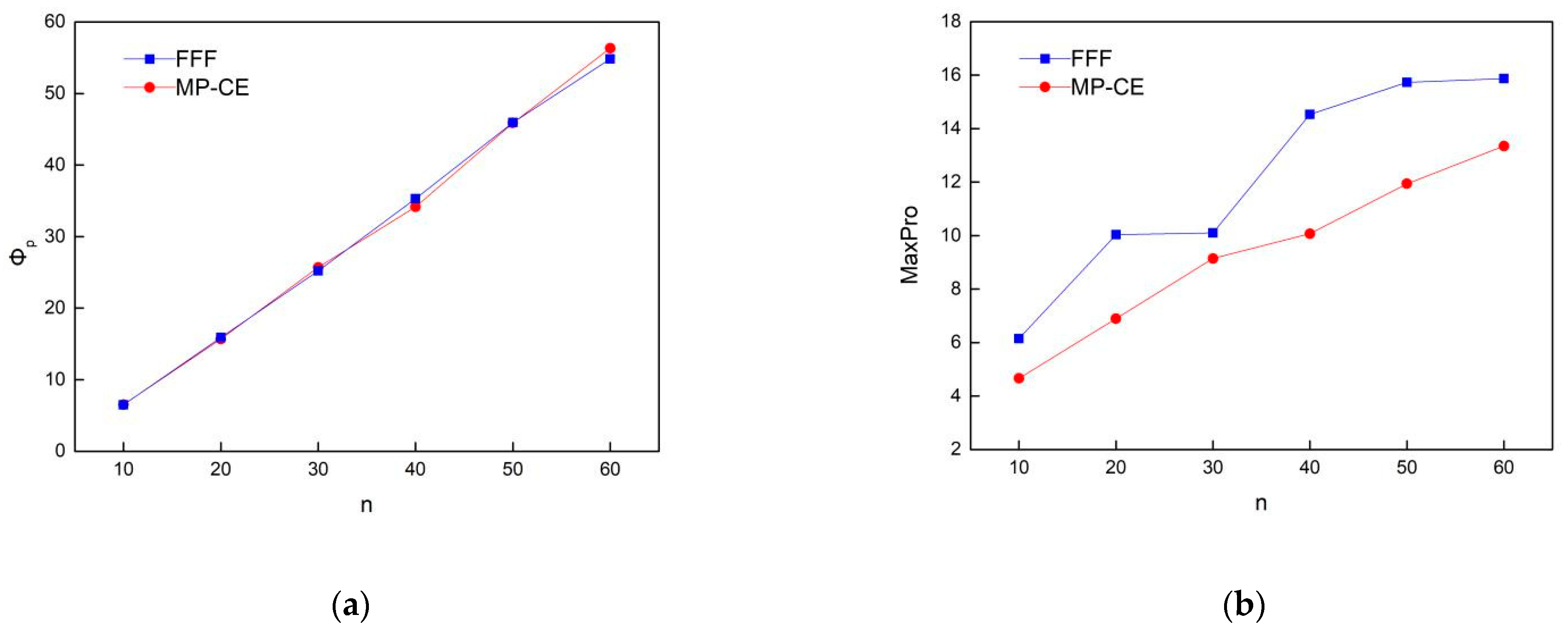
Experimental designs with different number of points were performed, as shown in Figure 5, leading to similar conclusions as described above. For the experimental design with multiple types of factors and complex constraints, MP-CE performs similarly to FFF in terms of space-filling distance but performs much better in terms of projection properties.

6. Conclusions

This paper proposes the MP-CE method to solve the problem of experimental design with multiple types of factors and complex constraints between factors. A coordinate selection strategy based on the projection property and distance property of design points is designed. By assigning probability of coordinate selection to overcome the shortcomings of randomness and easy to fall into local optimum and by adding perturbation to each local search of coordinate exchange, a new solution is explored in the areas where the exchange of coordinates may have an improvement, so as to retain the good features and attributes of the existing solution and avoid the shortcomings of random restart. The experimental results and analysis show that the MP-CE method is effective for experimental designs with multiple types of factors in complex constraints spaces, coupled with good performance in terms of space-filling properties.

References

- McKay, M.D.; Beckman. R.J.; Conover, W.J. Comparison of three methods for selecting values of input variables in the analysis of output from a computer code. Technometrics 1979, 21, 239–245. [Google Scholar]
- Johnson, M.E.; Moore, L.M.; Ylvisaker, D. Minimax and maximin distance designs. J. Stat. Plan. Inference 1990, 26, 131–148. [Google Scholar] [CrossRef]
- Fang, K.T. Uniform Design and Uniform Design Table; Science Press: Beijing, China, 1994. [Google Scholar]
- Joseph, V.R.; Gul, E.; Ba, S. Maximum projection designs for computer experiments. Biometrika 2015, 102, 371–380. [Google Scholar] [CrossRef]
- Qian, P. Sliced latin hypercube designs. J. Am. Stat. Assoc. 2012, 107, 393–399. [Google Scholar] [CrossRef]
- Zhang, J.; Xu, J.; Jia, K.; Yin, Y.; Wang, Z. Optimal sliced latin hypercube designs with slices of arbitrary run sizes. Mathematics 2019, 7, 854. [Google Scholar] [CrossRef] [Green Version]
- Ba, S.; Myers, W.R.; Brenneman, W.A. Optimal sliced latin hypercube designs. Technometrics 2015, 57, 479–487. [Google Scholar] [CrossRef]
- Deng, X.; Hung, Y.; Lin, C.D. Design for computer experiments with qualitative and quantitative factors. Stat. Sin. 2015, 25, 1567–1581. [Google Scholar] [CrossRef]
- Zhou, W.; Yang, J.; Liu, M.-Q. Construction of orthogonal marginally coupled designs. Stat. Pap. 2020, 62, 1–26. [Google Scholar] [CrossRef]
- Lekivetz, R.; Jones, B. Fast flexible space-filling designs with nominal factors for nonrectangular regions. Qual. Reliab. Eng. Int. 2019, 35, 677–684. [Google Scholar] [CrossRef]
- Huang, H.; Lin, D.K.; Liu, M.Q.; Yang, J.F. Computer experiments with both qualitative and quantitative variables. Technometrics 2016, 58, 495–507. [Google Scholar] [CrossRef]
- Joseph, V.R.; Gul, E.; Ba, S. Designing computer experiments with multiple types of factors: The MaxPro approach. J. Qual. Technol. 2020, 52, 343–354. [Google Scholar] [CrossRef]
- Draguljić, D.; Santner, T.J.; Dean, A.M. Noncollapsing space-filling designs for bounded nonrectangular regions. Technometrics 2012, 54, 169–178. [Google Scholar] [CrossRef] [Green Version]
- Beal, M.; Claeys, B.M. Constructing space-filling designs using an adaptive WSP algorithm for spaces with constraints. Chemom. Intell. Lab. Syst. 2014, 133, 84–91. [Google Scholar] [CrossRef]
- Kang, L. Stochastic coordinate-exchange optimal designs with complex constraints. Qual. Eng. 2018, 31, 401–416. [Google Scholar] [CrossRef]
- Lekivetz, R.; Jones, B. Fast flexible space-filling designs for nonrectangular regions. Qual. Reliab. Eng. Int. 2015, 31, 829–837. [Google Scholar] [CrossRef]
- Haaland, B.; Wang, W.; Maheshwari, V. A framework for controlling sources of inaccuracy in gaussian process emulation of deterministic computer experiments. SIAM/ASA J. Uncertain. Quantif. 2018, 6, 497–521. [Google Scholar] [CrossRef] [Green Version]
- Wang, W.; Haaland, B. Controlling sources of inaccuracy in stochastic kriging. Technometrics 2019, 61, 309–321. [Google Scholar] [CrossRef] [Green Version]
- Wang, W.; Tuo, R.; Wu, C.F.J. On prediction properties of kriging: Uniform error bounds and robustness. J. Am. Stat. Assoc. 2019, 115, 920–930. [Google Scholar] [CrossRef] [Green Version]
- Tuo, R.; Wang, W. Kriging prediction with isotropic Matern correlations: Robustness and experimental designs. J. Mach. Learn. Res. 2020, 21, 1–38. [Google Scholar]
- Jones, B. Computer Aided Designs for Practical Experimentation. Ph.D. Thesis, University of Antwerp, Antwerp, Belgium, 2008. [Google Scholar]
- Loureno, H.R.; Martin, O.C. Iterated local search: Framework and applications. In Handbook of Metaheuristics; Springer Science & Business Media: Berlin/Heidelberg, Germany, 2010. [Google Scholar]
- Cuervo, D.P.; Goos, P.; Sörensen, K. Optimal design of large-scale screening experiments: A critical look at the coordinate-exchange algorithm. Stat. Comput. 2016, 26, 15–28. [Google Scholar] [CrossRef]