Application of a Pattern-Recognition Neural Network for Detecting Analog Electronic Circuit Faults

Abstract

In this study, machine learning techniques based on the development of a pattern–recognition neural network were used for fault diagnosis in an analog electronic circuit to detect the individual hard faults (open circuits and short circuits) that may arise in a circuit. The ability to determine faults in the circuit was analyzed through the availability of a small number of measurements in the circuit, as test points are generally not accessible for verifying the behavior of all the components of an electronic circuit. It was shown that, despite the existence of a small number of measurements in the circuit that characterize the existing faults, the network based on pattern-recognition functioned adequately for the detection and classification of the hard faults. In addition, once the neural network has been trained, it can be used to analyze the behavior of the circuit versus variations in its components, with a wider range than that used to develop the neural network, in order to analyze the ability of the ANN to predict situations different from those used to train the ANN and to extract valuable information that may explain the behavior of the circuit.

1. Introduction

In analog electronic circuits, the limited access to measurement points makes determining faulty components a very complex task. On the other hand, when defining a set of measurement variables to characterize faults, many of the states that are generated by faults in the circuit are equivalent from the point of view of the values of the measured inputs, because the test points are generally not accessible to verify the behavior of all the components of the electronic circuit. In addition, performing measurements in each component of the circuit is not feasible from a practical point of view.

The present study deals with an application of supervised learning, based on the use of a pattern-recognition artificial neural network (ANN), for the detection of the individual hard faults (open circuits and short circuits) that may arise in an analog electronic circuit. The fact that the test points cannot be placed at all locations may cause several equivalent states to exist, depending on the points chosen to monitor the behavior of the circuit. This makes the detection of existing faults in an analog circuit a very complex task and much less developed than the same task in digital electronic circuits. In order to detect the hard faults that may arise in an electronic circuit, measurements are to be taken at accessible points in the circuit. Specifically, for the analysis to be carried out in this study, measurements of DC voltage and voltage gain were considered as input values so that it was possible to monitor the circuit and to determine, from these easily obtainable measures, whether the circuit was in a hard fault situation (open circuit or short circuit).

The first circuit under test (CUT) used in the present study was a single-stage small-signal BJT amplifier, in which it is difficult to detect the hard faults that may arise because some faults lead to an equivalent state, from the point of view of the inputs used to monitor the behavior of the circuit, and later a more complex CUT was also studied. First, in the present study, the outputs of the CUTs versus variations that may arise from the tolerances of the passive elements of the circuit were obtained through a Monte Carlo analysis by using Cadence^® OrCAD^® (CA, USA) design electronic simulation software. The values thus obtained were then used to train the ANN applied to predict the faulty components of the circuit. Moreover, a dataset obtained from the simulation software was used to validate and test the obtained results. In addition, once the pattern-classification neural network had been obtained, it was used to predict the behavior of the circuit subject to variations in the faulty components at wider ranges than those used to develop the neural network. This was carried out to determine the ranges of the parameters from which it is possible to detect hard faults in the CUTs.

Nowadays, determining faults in analog electronic circuits is being deeply studied by several research studies. For example, as shown in a review of Binu and Kariyappa [1], fault diagnosis in electronic circuits has been extensively researched in the last few years, for which machine learning approaches have been widely applied for fault detection. As shown by Binu and Kariyappa [1], open circuits and short circuits are some of the main failure sources in analog electronic circuits, and these hard faults can be modeled by including a 1 Ω parallel resistance with the component in a short-circuit situation and a 1 MΩ series resistance with the component in an open-circuit situation.

As previously mentioned, fault diagnosis in analog electronic circuits is a very complex task and is much less developed than the equivalent task in digital electronic circuits. The methods for analyzing faults in analog electronic circuits may be classified, roughly speaking, into two main categories: simulation before test (SBT) and simulation after test (SAT), as shown in the research study of Aizenberg et al. [2].

In the SBT approach, the development of a fault dictionary is very useful for detecting the faults in a circuit. In that way, the main faults that may arise in the circuit are simulated along with the nominal behavior of the circuit. In addition, in order to detect the faults that can occur in the analog circuit, it is important to consider both ambiguity groups, that is, the set of components of the electronic circuit that do not provide a unique solution if considered as a potential fault, and the canonical ambiguity groups, where a canonical ambiguity group is a group that does not contain other ambiguity groups [2,3,4], because it is very difficult to determine which component is faulty within one of these ambiguity groups.

Over the last few years, soft computing techniques for modeling and analyzing the behavior of electronic devices, as well as other kind of devices, have been widely used. As a consequence, several research studies dealing with this subject have been developed, as can be observed, for example, in [5,6,7,8,9], among many others research studies. With regard to the application of ANNs for detecting faults in analog electronic circuits, the study of Gao et al. [10] could be mentioned, where a dual-input fault diagnosis model based on convolutional neural networks, gated recurrent unit networks, and a softmax classifier was proposed. Likewise, Zhang et al. [11] used a convolutional neuronal network and backward difference for soft fault diagnosis in analog circuits, where the circuits being tested were the Sallen–Key band-pass filter and a four-opamp biquad high-pass filter.

Another studyworth mentioning is that of Wang et al. [12], which used a long short-term memory neural network for fault detection and classification in modular multilevel converters in high-voltage direct current systems.

On the other hand, Xiao and Feng [13] used Monte Carlo analysis and SPICE simulation along with particle swarm optimization to tune the neural networks for analog fault diagnosis. Likewise, Aizenberg et al. [2] presented a method for detecting single parametric faults in analog circuits. They used a multi-valued neuron-based multilayer neural network (MLMVN) as a classifier, and a comparison with support vector machines (SVMs) was also presented in their study. These authors found that the MLMVN was highly accurate for classifying the fault class (FC) in the circuits under analysis in their study. Likewise, in the research of Kalpana et al. [14], Monte Carlo analysis was combined with machine learning techniques for fault diagnosis in analog circuits based on SBT.

Neural networks and genetic algorithms were also used in Tan et al. [15] for analog fault diagnosis, in which PSPICE simulations were used, and three different circuits were analyzed. These authors applied back propagation neural networks with 28–36 hidden layers, depending on the CUT, and with a binary coding scheme for the outputs, where the open-circuit faults were modeled with 1 × 10⁶ times the nominal parameters and the short circuit as 1 × 10⁻⁶ the nominal values of each element. On the other hand, Viveros-Wacher et al. [16] used a CMOS RF negative feedback amplifier as the CUT for diagnosing faults using ANNs.

Some other studies on diagnosing analog circuit faults used neural networks and fuzzy logic, as shown by Bo et al. [17], who used a negative feedback amplifier as the CUT. Simulation and deep learning were also used by Pawlowski et al. [18] for identifying circuit faults in post-market circuit boards. In other studies, Li et al. [19] used a radial basis function (RFB) neural network and a back propagation algorithm for fault detection in a differential amplifier circuit. An RBF and back propagation were also used by Wuming and Peiliang [20], who employed a particle swarm optimization algorithm to adjust the neural network. SPICE and a quantum Hopfield neural network were employed by Li et al. [21] for fault analysis in a Sallen–Key band pass filter. Likewise, Monte Carlo analysis combined with deep learning and convolutional neuronal networks were used in Moezi and Kargar [22] for fault detection in analog circuits. In another study, Mosin [23] applied a three-layer feedforward neural network for fault diagnosis, where a tan-sigmoid function was used as the transfer function for the input and intermediate layers, and a log-sigmoid function was employed for the output layer, with a Sallen–Key bandpass filter being the CUT.

Further studies are that of Grasso et al. [24], which applied a procedure based on multifrequency fault diagnosis, where the CUT was a two-stage CE audio amplifier, and that of Li and Xie [25], which used a method based on the cross-entropy between a circuit under nominal behavior and one with faults, where the CUT was analyzed by Monte Carlo simulation. Some other studies are that of Sheikhan and Sha’bani [26], which used a modular neural model for soft fault diagnosis in analog circuits; that of Liang et al. [27], which applied a support vector machine classifier and fuzzy feature selection for analog circuit fault diagnosis; and that of Wang et al. [28], which used a semi-supervised algorithm for parametric fault diagnosis in analog circuits, among many others.

The remainder of this article is structured as follows: In Section 2, the methodology used to develop the ANN used to detect circuit faults is shown. In Section 3, the results are presented. A discussion of these results is provided in Section 4. Finally, the main conclusions of this study are outlined in Section 5.

2. Fault Diagnosis Method

As previously mentioned, this study analyzed the application of a pattern-classification ANN to detect hard faults in two analog circuits in which the faults that could arise were difficult to diagnose because several faults could provide similar results, from the point of view of the selected test points used to monitor the behavior of the circuit, because the test points should be selected in accessible points of the circuit and cannot simply be located anywhere due to practical considerations. Therefore, to detect the faults that may arise in the circuit, three measurements of DC voltage and the gain voltage were considered as input variables in the first CUT and six measurements of DC voltage and the gain voltage were considered as input variables in the second one. In order to develop the ANN used in this study, the software Cadence^® OrCAD^® Design Systems was first used in order to carry out a Monte Carlo analysis of the tolerances of the passive components of the circuit. 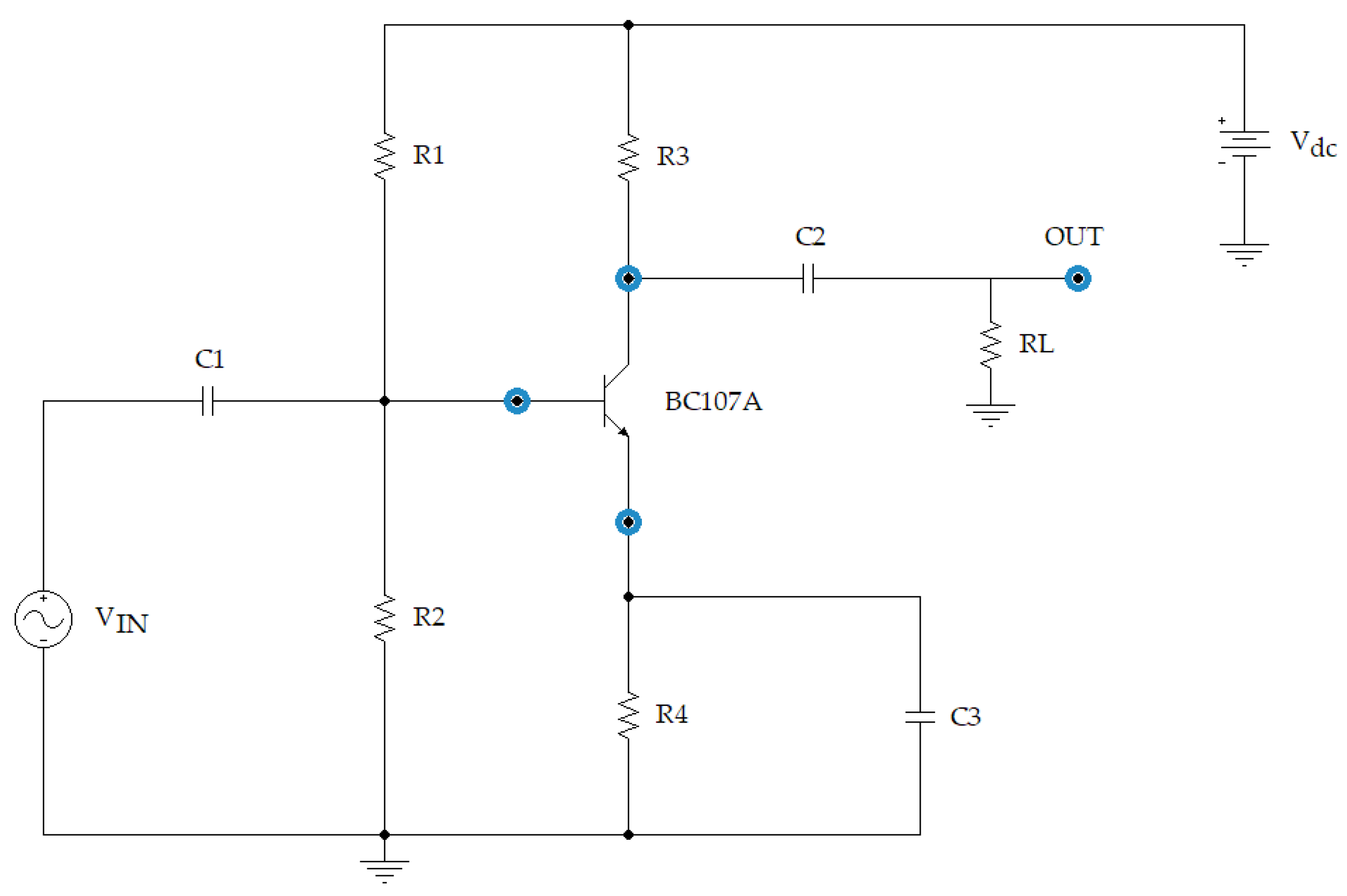The first CUT is shown in Figure 1, for which it is assumed that only the DC voltage in the transistor and the gain voltage are available. In addition, a simulation was first used to determine the failure situations that presented ambiguity because it was not possible to determine precisely which was the faulty component.

Figure 1 shows the first CUT used in the present study, which is a single-stage small-signal BJT amplifier, similar to that shown in [29]. Likewise, Figure 1 shows the test points in this study. As can be observed, these test points are easily accessible. The nominal values of the circuit’s components are shown in

Table 1. Nominal values and tolerances of the passive components of the circuit.

	R1 (kΩ)	R2 (kΩ)	R3 (kΩ)	R4 (kΩ)	C1 (μF)	C2 (µF)	C3 (μF)
Nominal value	15	2.7	5.6	1.8	82	10	56
Tolerance	10%	10%	10%	10%	20%	20%	20%

and

Table 2. Values of the load resistance and voltage sources of the circuit.

VIN (Sinusoidal Voltage Source)	Vdc (Power Supply)	RL (Load Resistance)
VINmax = 10 mV; frequency = 1 kHz	20 V	8.2 kΩ

. First, the application of the pattern-recognition ANN to the CUT shown in Figure 1 is analyzed, and later, a more complex circuit that incorporates two amplification stages is analyzed in order to show that the ANN developed is capable of adequately predicting fault situations, as well as nominal behavior, in the second CUT.

Table 3. Nominal behavior and hard faults grouped by ambiguity groups (M_j classes).

M01	M02	M03	M04	M05	M06	M07	M08	M09	M10	M11
F01	F13	{F02, F05, F11}	{F10, F12}	F14	{F09, F15}	F07	F08	F03	F04	F06
Nominal	C2sc	{R1oc, R2sc, C1sc}	{C1oc, C2oc}	C3oc	{R4sc, C3sc}	R3sc	R4oc	R1sc	R2oc	R3oc

shows the possible individual faults that may arise in the first CUT obtained when the hard faults (a short circuit (sc) or an open circuit (oc)) arise in the passive components. From Table 3, it is possible to see that, in this CUT, there are 14 individual hard faults, as well as the nominal behavior of the circuit {Nominal, R_1oc, R_1sc, R_2oc, R_2sc, R_3oc, R_3sc, R_4oc,R_4sc, C_1oc, C_1sc, C_2oc, C_2sc, C_3oc, C_3sc}, which were coded as {F₀₁, F₀₂, F₀₃, F₀₄, F₀₅, F₀₆, F₀₇, F₀₈, F₀₉, F₁₀, F₁₁, F₁₂, F₁₃, F₁₄, F₁₅ }. Therefore, these were the working modes that were analyzed. As previously mentioned, in order to characterize the behavior of the CUT, an electronic simulation was carried out by using Cadence^® OrCAD^® design electronic simulation software for each of the failure modes shown in Table 3. As can be observed, the faults were grouped into ambiguity groups, from the point of view of the inputs considered to diagnose the circuit’s behavior, where a hard fault in a component of the circuit due to an open circuit (oc) was simulated by placing a resistance (R_Fault = 10 MΩ) in series with the component, and a hard fault due to a short circuit (sc) was simulated by placing a resistance (R_Fault = 1 Ω) in parallel with the component. The ambiguity groups were determined from the values of the inputs, which were obtained from an electronic simulation. These ambiguity groups (M_j classes) were coded as {M₀₁, M₀₂, M₀₃, M₀₄, M₀₅, M₀₆, M₀₇, M₀₈, M₀₉, M₁₀, M₁₁}. It should be mentioned that there are some fault events, such as those obtained, for example, in the M₀₄ class, which include hard faults {F₁₀, F₁₂}, in the event of which it would not be possible to determine the faulty component. Moreover, in case of a situation due to a catastrophic fault leading to an actual open circuit or a short circuit, the DC voltages and the gain voltage (Av) could be different from those obtained by the model employed in this study. These situations were obtained from the simulation when a 10 MΩ resistance was placed in series with the faulty component to simulate the open circuit (oc), and when a value of 1 Ω resistance was placed in parallel with the faulty component. Therefore, to consider the actual catastrophic fault, the values obtained in the test points were also obtained from the simulation and considered as additional inputs to those provided by the Monte Carlo analysis in order to train the ANN.

A Monte Carlo analysis considering the tolerances of the passive elements of the circuit shown in Table 1 was first carried out for each of the hard faults (open circuits and short circuits) in order to train the ANN, and 64 results were generated for each fault (63 results from the Monte Carlo analysis and 1 additional result from the actual catastrophic fault). Likewise, 64 results were obtained for the nominal behavior. These results were then used to train the pattern-recognition ANN considered in this study. Figure 2 shows the ANN applied, which was trained to detect the nominal behavior and the individual faults shown in Table 3. The hard faults that may arise in the circuit shown in Figure 1, as well as the nominal behavior, were characterized from the outputs of the ANN as shown in Equation (1):

$$S_j=colum{n}_{j-th}\left\{I\right\}$$

(1)

where $S_j$ corresponds to the ANN outputs, so that the j-th output class corresponds to the j-th column of the identity matrix $\left(I\right)$. The nominal behavior corresponds to $M_{01}\left(F_1\right)$ and the remaining classes shown in Table 3 correspond to the short-circuit and open-circuit faults, where the hard faults were grouped by the ambiguity groups obtained from the inputs used to characterize the behavior of the circuit. Therefore, the coding used to characterize a fault should provide a “1” in the position of the fault and “0” in the rest of the outputs, and hence, all outputs will have a “0” value except the j-th class (the fault class to be identified), which will have a “1” value. The same is applicable for the nominal value.

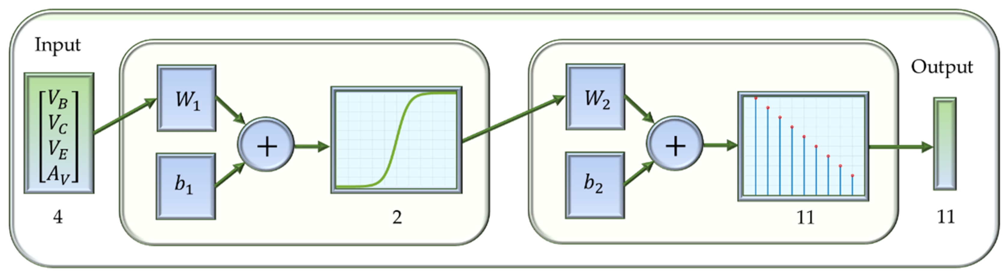
As can be observed, in Figure 2, the first ANN used in the present study was made up of an input layer that has four inputs (V_B, V_C, V_E, A_V), which correspond to the DC voltages in the base, collector, and emitter of the BJT transistor and to the gain voltage (A_V), respectively, as well as a single hidden layer (with two neurons and a hyperbolic tangent as the transfer function) and one output layer with a softmax transfer function, which is commonly used in pattern-recognition neural networks. As can be noted, the output layer has 11 outputs, which correspond to the 10 fault classes identified in the electronic circuit and to the nominal working mode.

As shown later in this study, with the configuration given in Figure 2, it is possible to have high accuracy in the ANN for detecting both the hard faults of the circuit and the nominal behavior. It should be mentioned that different ANN topologies were analyzed with one and two hidden layers and by using different training algorithms to adjust the ANN parameters. Finally, a Levenberg–Marquardt back propagation algorithm was selected to update the weights and biases of the ANN by using the Deep Learning Toolbox™ of MATLAB^TM 2020a [30]. The ANN shown in Figure 2 was used, since it was able to provide accurate results without having to increase the number of neurons or the number of hidden layers. The metric used to test the models was the mean squared error (MSE). Different transfer functions were also analyzed in the hidden layer but, finally, a hyperbolic tangent was used in this study. On the other hand, the Levenberg–Marquardt algorithm was able to provide, in this case, more accurate results than the others analyzed, such as the Scaled Conjugate Gradient. Therefore, the topology was that shown in Figure 2, where $W_1$ and $b_1$ are the weights and bias of the hidden layer, and $W_2$ and $b_2$ are those of the output layer. As previously mentioned, a hyperbolic tangent $(f_1)$ was used as the transfer function in the hidden layer and a softmax transfer function $(f_2)$ was used in the output layer.

$$Outputs=f_2\left(W_2\ast f_1\left(W_1\ast Inputs+b_1\right)+b_2\right)$$

(2)

As Figure 2 shows, the number of outputs was 11, where each output corresponds to the class identified (Mj); one of them represents the nominal behavior and the remaining classes representing the ambiguity groups, where the outputs of the ANN can be obtained from Equation (2). In order to obtain the results shown in this study, the Deep Learning Toolbox^TM of MATLAB^TM R2020a [30] was used.

3. Results

After training the ANN shown in Figure 2 with the data obtained from the Monte Carlo simulations and following the procedure shown in the previous section, it was possible to obtain the confusion matrices shown in Figure 3, Figure 4, Figure 5 and Figure 6, for training, validation, testing, and all data, respectively, where 70% of data were used for training, 15% for testing and 15% for the validation. As can be observed, in Figure 3, Figure 4, Figure 5 and Figure 6, a perfect classification of the results was obtained with this ANN comprising a single hidden layer that contains two neurons.

Figure 3 shows the results obtained in the confusion matrix when 70% of the data from the Monte Carlo analysis were employed to train the ANN. It can be seen that there are fault classes that present a larger amount of data due to the fact that they agglutinate fault configurations that belong to the same ambiguity group. As can be seen, 100% of the data are classified correctly.

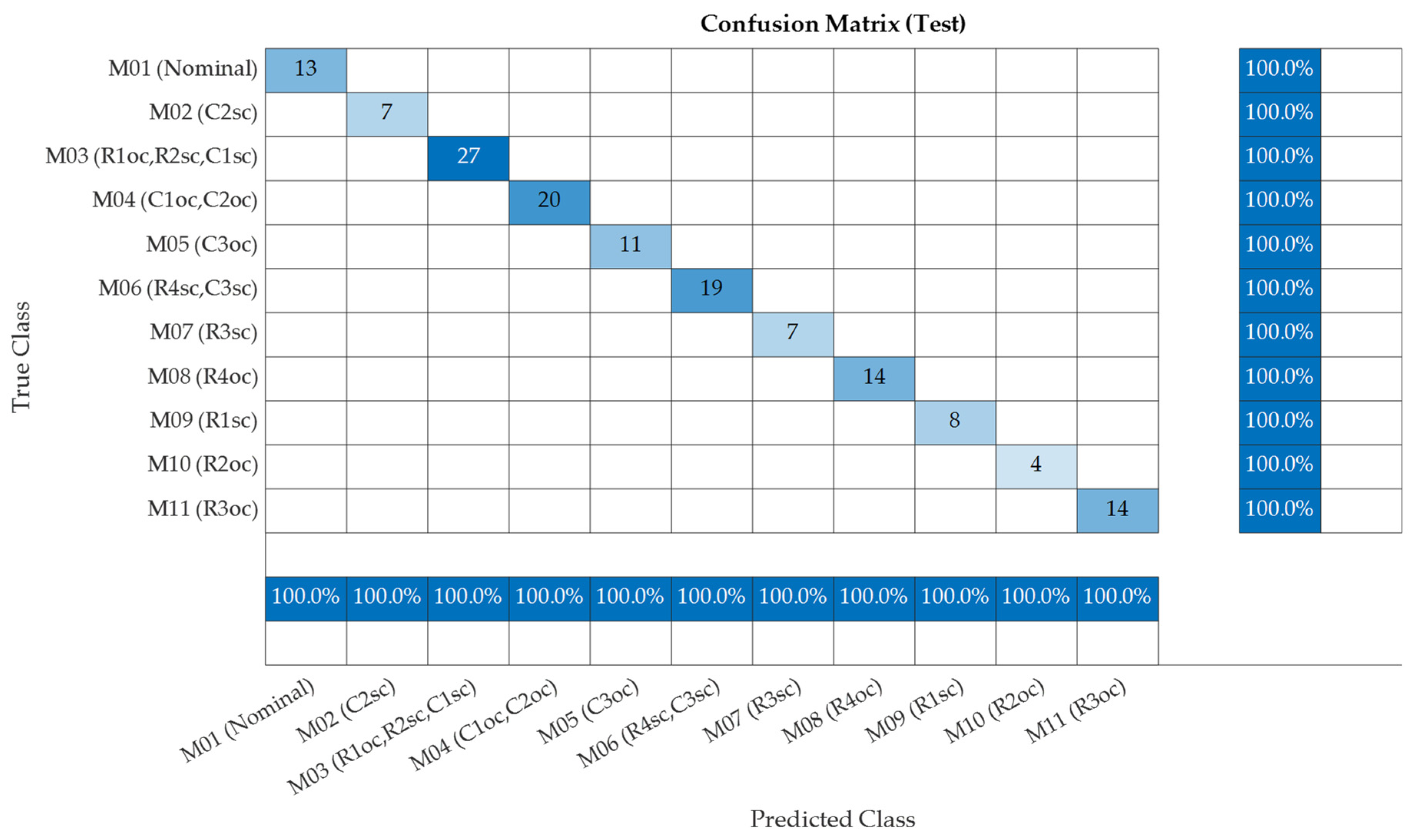
Figure 4 shows the results obtained in the confusion matrix when 15% of the Monte Carlo data were used for validation of the ANN, and Figure 5 shows the results for the test case. Similar to the results obtained during training, the ANN was able to diagnose 100% of the working modes correctly (hard faults and nominal behavior).

Figure 6 shows the results of the confusion matrix for each of the hard faults and for the nominal behavior considering all the Monte Carlo data. As previously mentioned, 64 values were used for each fault and for the nominal behavior in the Monte Carlo analysis by considering the tolerances of the components.

It can be noted in Figure 6 that, in the confusion matrix generated from all data, there are classes with a greater number of elements because the ambiguous failure modes were grouped into failure classes. Thus, for example, class M₀₃ has 192 elements, since it encompasses three failure modes (R_1oc, R_2sc, C_1sc). In addition, it can be seen that 100% of the data were classified correctly.

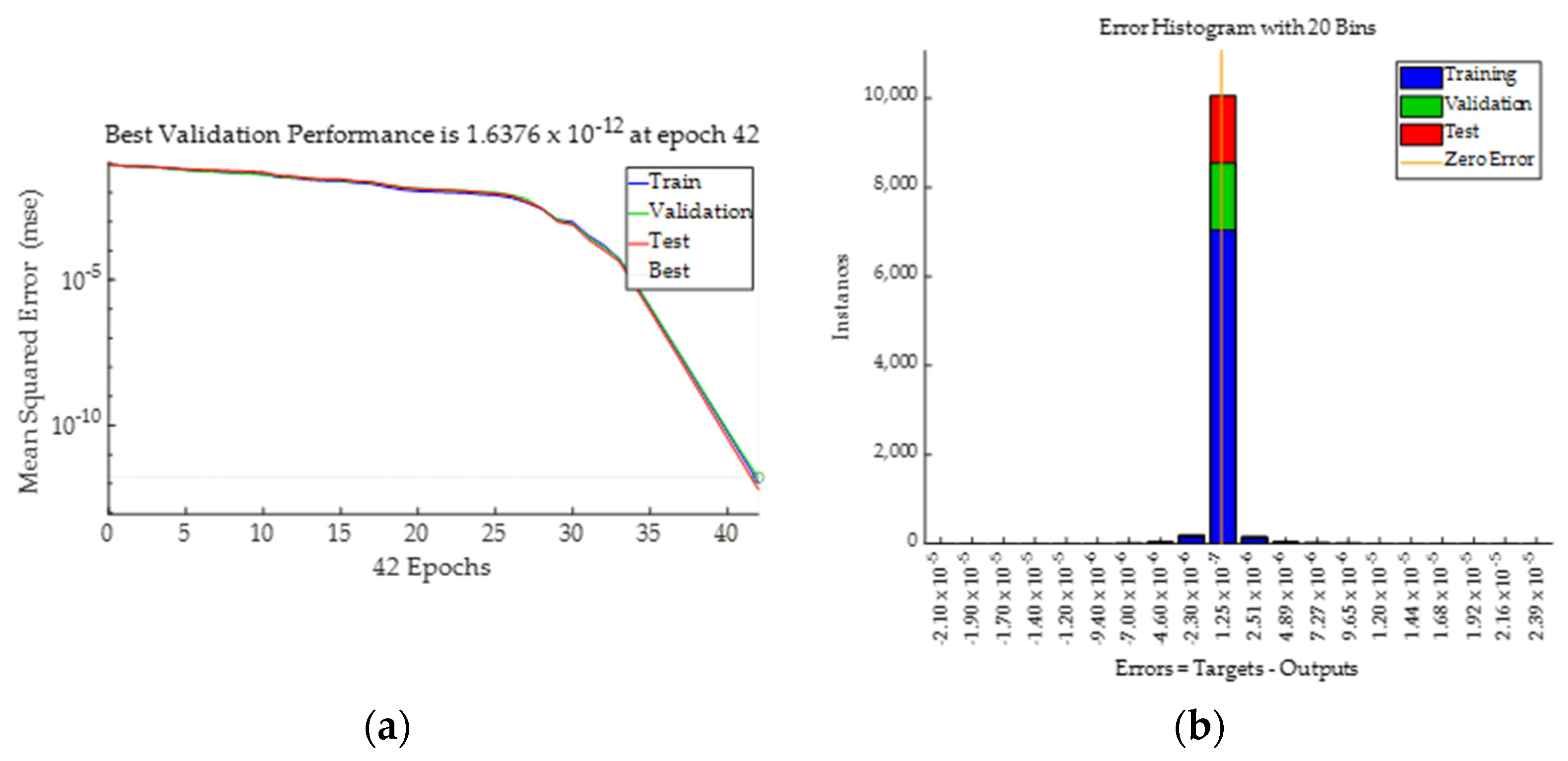
Figure 7a shows the mean squared error (MSE) obtained with the ANN and Figure 7b shows the error histograms for training, validation, and testing.

As Figure 8 shows, the ROC (receiver operating characteristic) curves have an area under the curve (AUC) of 1, which demonstrates that the pattern-recognition ANN developed was able to diagnose the working modes of the BJT amplifier once they were classified into the 11 classes shown in Table 3. In order to show that the pattern-recognition ANN is capable of predicting the behavior of other circuits, a two-stage small-signal BJT amplifier, such as that shown in Figure 9, was also analyzed in the present study.

The nominal values of the circuit’s components are shown in

Table 4. Nominal values and tolerances of the passive components of the circuit (R).

	R1 (kΩ)	R2 (kΩ)	R3 (kΩ)	R4 (kΩ)	R5 (kΩ)	R6 (kΩ)	R7 (kΩ)	R8 (kΩ)
Nominal value	15	2.7	5.6	2.2	15	2.7	7.5	1.8
Tolerance	10%	10%	10%	10%	10%	10%	10%	10%

,

Table 5. Nominal values and tolerances of the passive components of the circuit (C).

	C1 (μF)	C2 (µF)	C3 (μF)	C4 (µF)	C5 (μF)
Nominal value	100	1	0.56	10	47
Tolerance	20%	20%	20%	20%	20%

and

Table 6. Values of the load resistance and the voltage sources of the circuit.

VIN (Sinusoidal Voltage Source)	Vdc (Power Supply)	RL (Load Resistance)
VINmax = 1 mV; frequency = 1 kHz	20 V	8.2 kΩ

.

Table 7. Nominal behavior and hard faults in the second CUT grouped by ambiguity groups (M_j classes).

M01	M02	M03	M04		M05	M06		M07	M08	M09
Nominal	C2sc	{R1oc, R2sc, C1sc}	{C1oc, C2oc, C4oc}		C3oc	{R4sc, C3sc}		R3sc	R4oc	R1sc
M10	M11	M12	M13	M14	M15	M16	M17	M18	M19	M20
R2oc	R3oc	{R8sc, C5sc}	{R5oc, R6sc}	C4sc	C5oc	R5sc	R6oc	R7oc	R7sc	R8oc

shows the possible individual faults that may arise in the second CUT obtained when the hard faults (short circuit (sc) or open circuit (oc)) arise in the passive components. From Table 7, it is possible to see that, in this second CUT, there are 27 individual hard faults, as well as the nominal behavior of the circuit {nominal, C_1oc, C_1sc, C_2oc, C_2sc, C_3oc, C_3sc, C_4oc, C_4sc, C_5oc, C_5sc, R_1oc, R_1sc, R_2oc, R_2sc, R_3oc, R_3sc, R_4oc, R_4sc, R_5oc, R_5sc, R_6oc, R_6sc, R_7oc, R_7sc, R_8oc, R_8sc }, which were coded as {F₀₁, F₀₂,…, F₂₆, F₂₇}, where F₀₁ corresponds to the nominal behavior. Therefore, these are the working modes that are analyzed in the second case. As can be observed, the faults were grouped into ambiguity groups, from the point of view of the inputs considered to diagnose the circuit’s behavior, following the previously mentioned procedure, where a hard fault in a component of the circuit due to an open circuit (oc) was simulated by placing a resistance (R_Fault = 10 MΩ) in series with the component, and a hard fault due to a short circuit (sc) was simulated by placing a resistance (R_Fault = 1 Ω) in parallel with the component.

As in the previous case, the ambiguity groups were determined from the values of the inputs, which were obtained from an electronic simulation. These ambiguity groups (M_j classes) were coded as {M₀₁, M₀₂, …, M₁₉, M₂₀} because, in this second case, 20 classes were detected. It should be mentioned that there are some fault events, such as those obtained, for example, in the M₀₃ class, that include hard faults {R_1oc, R_2sc, C_1sc} for which it would not be possible to determine the faulty component. Moreover, in case of a situation due to a catastrophic fault leading to an actual open circuit or a short circuit, the DC voltages and the gain voltage (Av) could be different to those obtained by the model employed in this study. Therefore, to consider an actual catastrophic fault, as in the previous case, the values obtained in the test points were also obtained from the simulation and considered as additional inputs to those provided by the Monte Carlo analysis in order to train the ANN.

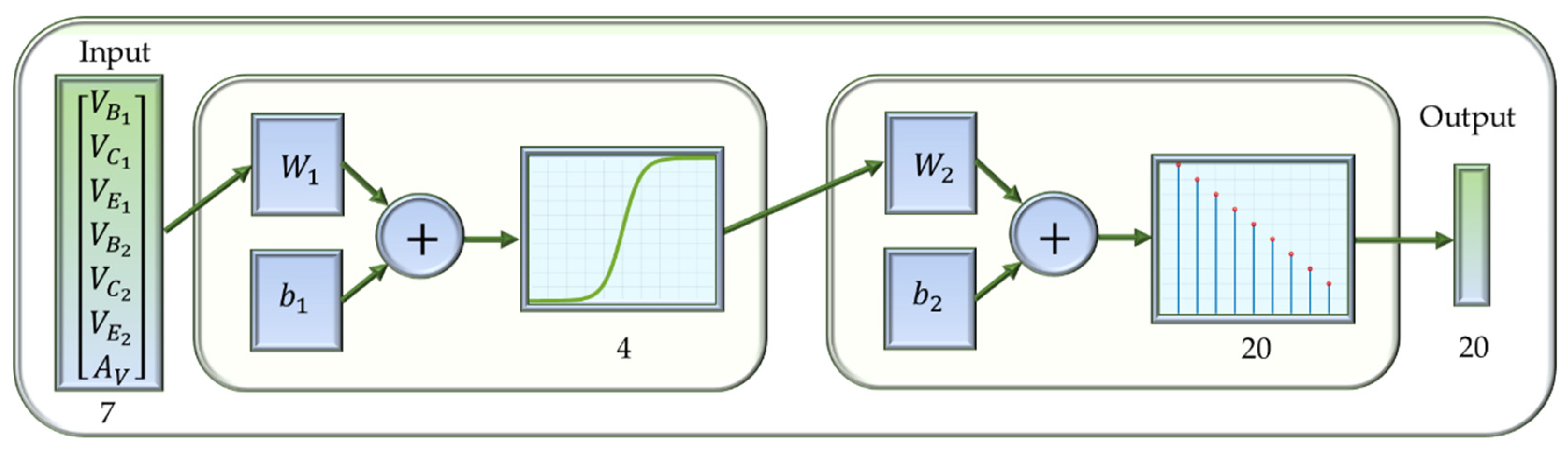
Figure 10 shows the ANN for the second CUT, which is shown in Figure 9. As can be seen in this case, the number of inputs is seven, which correspond to the voltages at the base, emitter and collector of both transistors as well as the gain voltage (V_B1, V_C1, V_E1, V_B2, V_C2, V_E2, A_V), and the outputs are 20, corresponding to the detected fault classes and the nominal behavior. Similar to the previous case, the same network topology is used, although, in this case, there are four neurons in the hidden layer. As was done with the ANN developed for the first CUT, a Levenberg–Marquardt back propagation algorithm was selected to update the weights and biases of the ANN by using the Deep Learning Toolbox™ in MATLAB^TM 2020a [30].

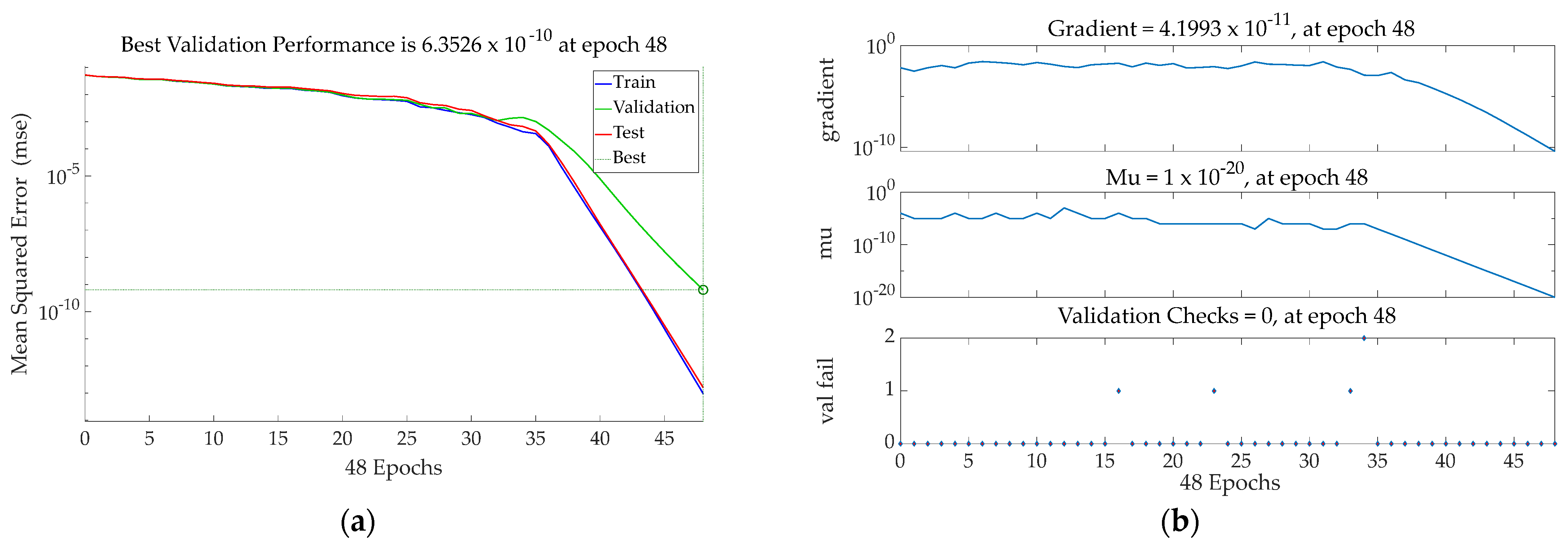
Figure 11a shows the MSE values obtained versus the number of epochs, and Figure 11b shows the training state values for the ANN employed to analyze the faults in the second CUT.

Figure 12 shows the results obtained in the confusion matrix when 70% of the data from the Monte Carlo analysis were employed to train the ANN shown in Figure 10, which was employed to model the behavior of the second CUT. It can be seen that there are fault classes that present a larger amount of data due to the fact that they agglutinate fault configurations that belong to the same ambiguity group. As can be seen, 100% of the data are classified correctly in the second case, similar to the previous one. As can be observed, the fault classes do not have the same number of elements because the data used to train, validate, and test the ANN were randomly selected.

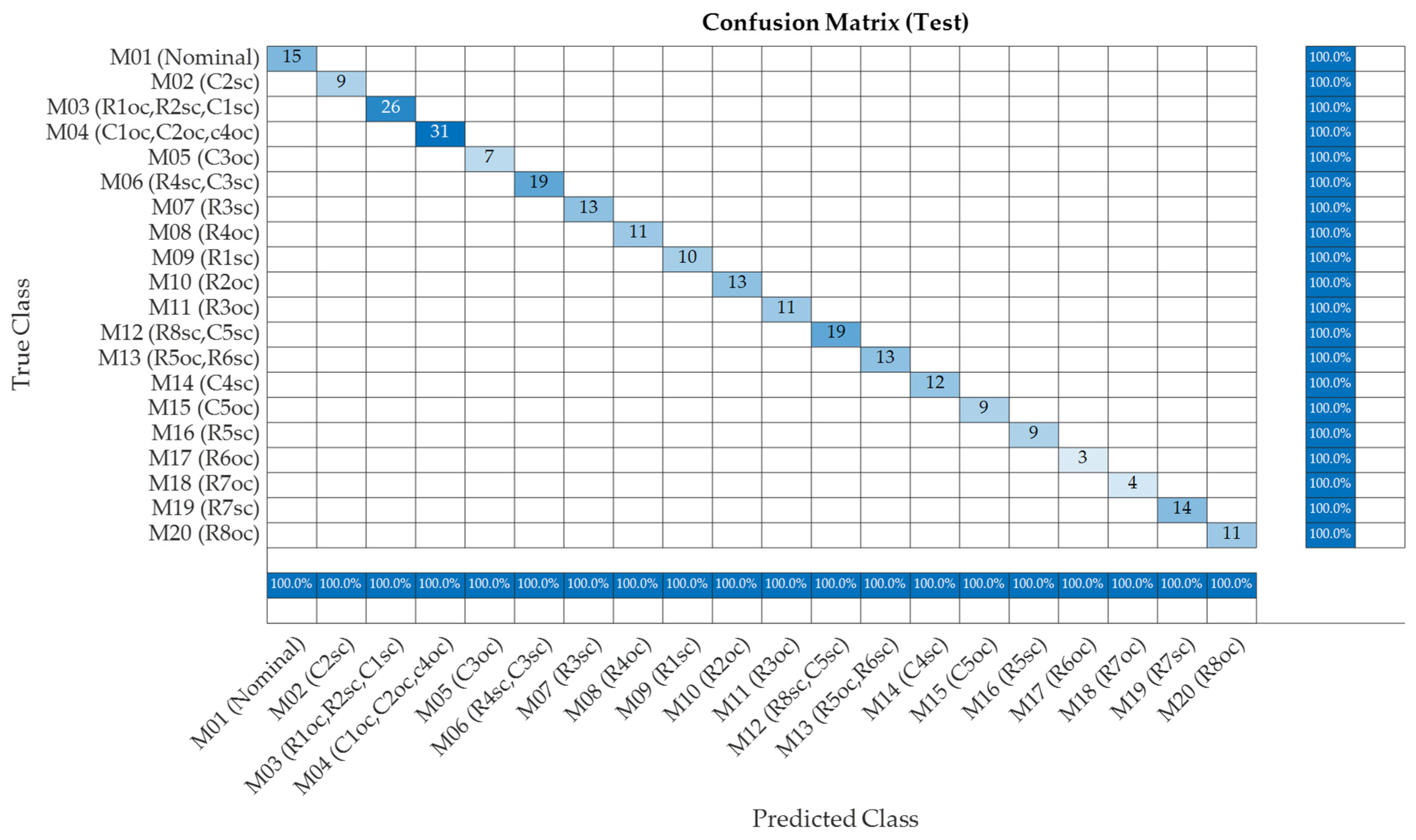
Figure 13 shows the results obtained in the confusion matrix when 15% of the Monte Carlo data were used for validation of the ANN, and Figure 14 shows the results for the test case. Similar to the results obtained during training, the ANN was able to diagnose 100% of the working modes correctly (hard faults and nominal behavior). As can be observed, the same results as those obtained with the first CUT were obtained with the second CUT.

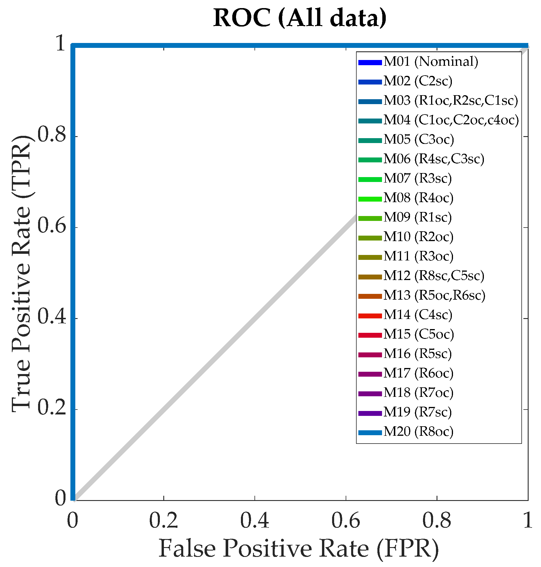
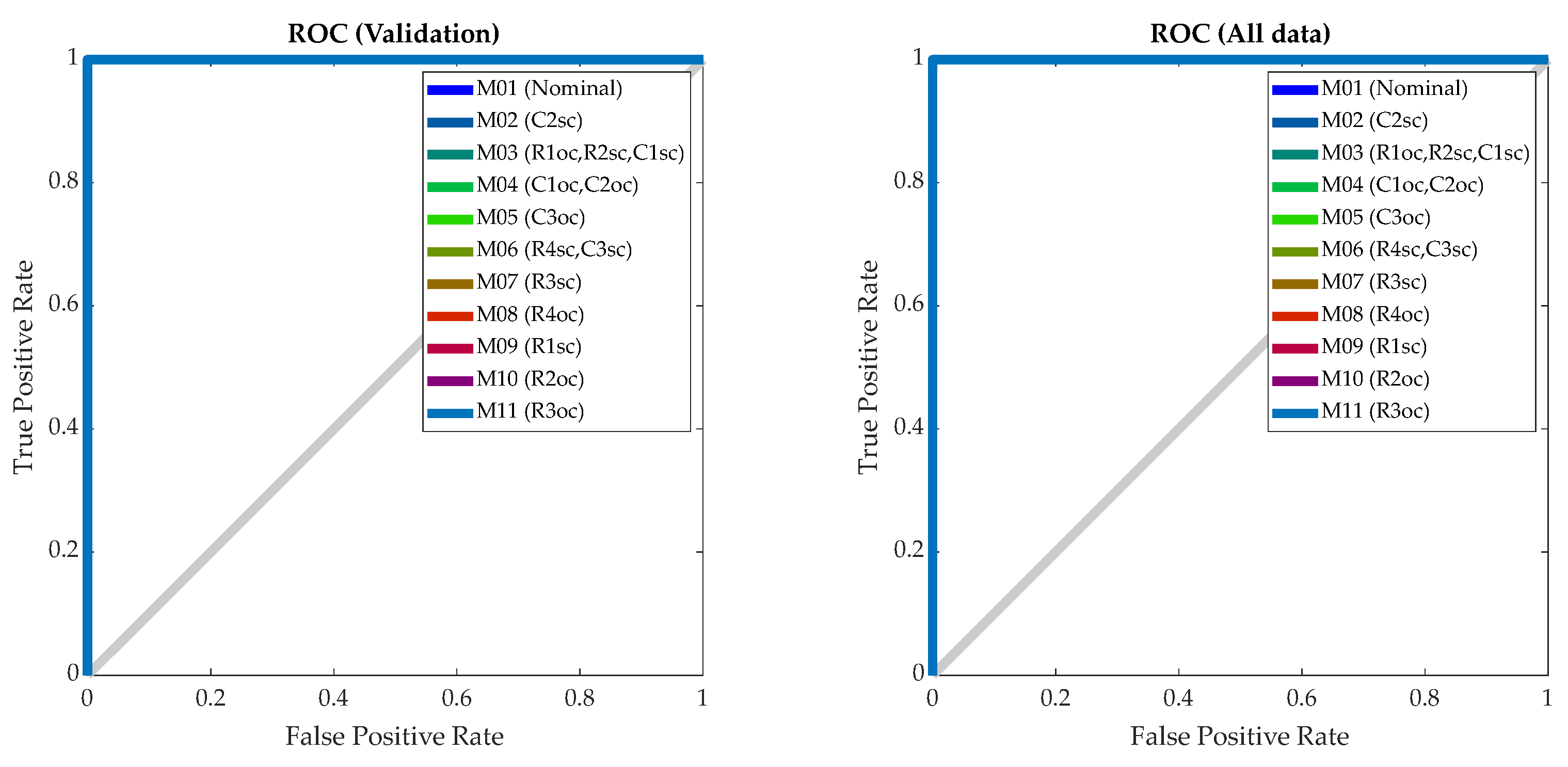
Finally, Figure 15 shows the confusion chart for all data, and Figure 16 shows the ROC curve (all data) for the second CUT. In this curve, the true positive rate (TPR) versus the false positive rate (FPR) was plotted at different threshold settings. The ANN developed in this study is a perfect classifier for the electronic faults in the second CUT because it is perfectly able to distinguish each fault class for any FPR. Similar to the results obtained with the first CUT, it can be seen that 100% of the data were classified correctly.

4. Discussion

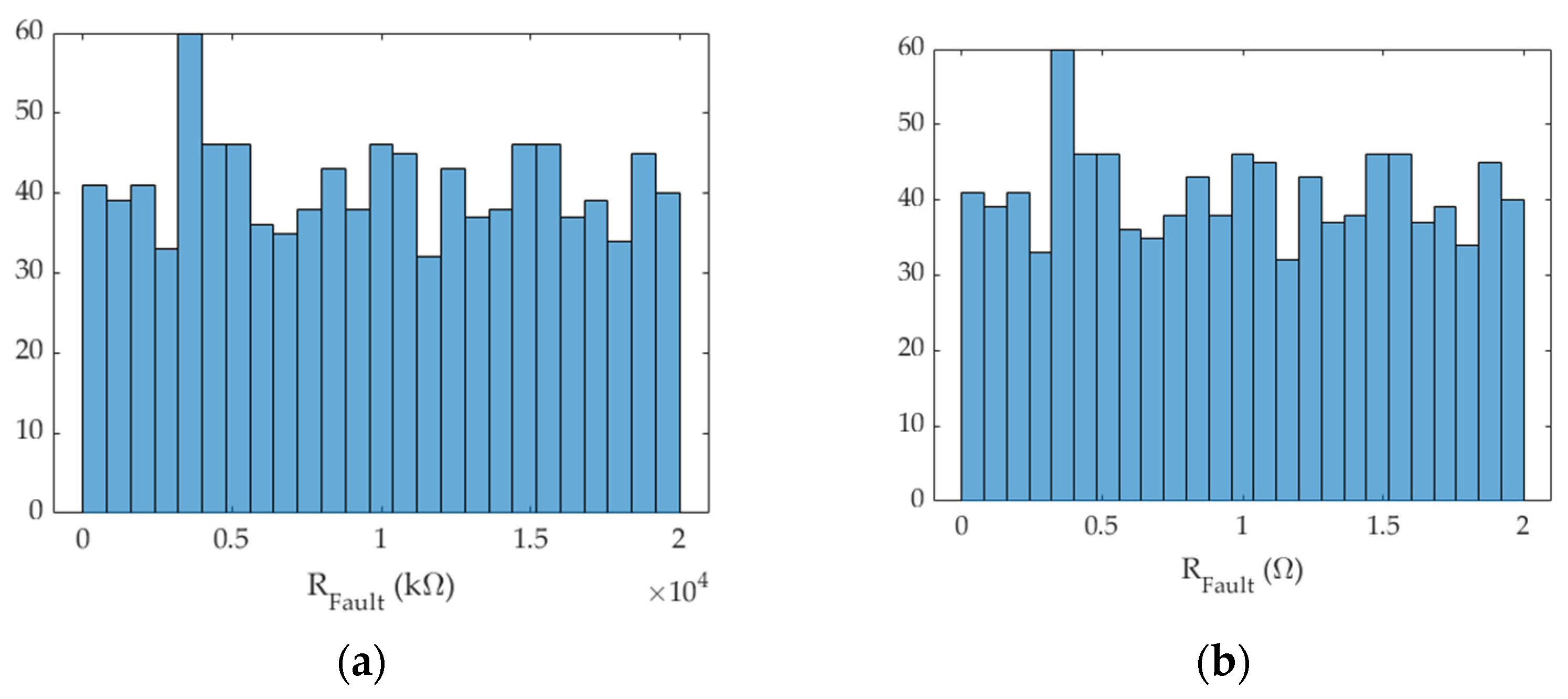
As Figure 8 and Figure 16 show, the pattern-recognition ANN can correctly diagnose both the nominal behavior and the fault classes of the CUTs considered in the present study, with 100% of the data correctly classified when considering 64 Monte Carlo points for each fault and for the nominal behavior. However, in order to analyze the ability of the ANN to explain situations different from those used to train the ANN and to extract valuable information that may explain the behavior of the circuit, wider ranges of the fault resistances placed in series and in parallel with the components to simulate the hard faults in the CUT were used. These values were chosen in order to generate different fault scenarios to determine the ability of the developed ANN to diagnose possible fault situations before a hard fault occurs. To test the ANN with these fault resistances, a new Monte Carlo analysis was performed. In this later case, the number of runs generated for the fault resistance was 1024, for each fault, instead of the 64 runs used to train the ANN, following a uniform distribution, as shown in Figure 17a, for the case of a fault resistance in series with the faulty component to simulate an open circuit, and in Figure 17b for the case of a fault resistance in parallel with the faulty component to simulate a short circuit. On the other hand, the rest of the components of the CUT were allowed to vary within the specified tolerances.

That is, to train the neural network, an initial Monte Carlo analysis was performed for the CUT in which 64 runs were used for each fault event as well as for the nominal value. This results in a total of 960 input vectors (V_B, V_C, V_E, A_V) in the case of the first CUT and a total of 1728 input vectors (V_B1, V_C1, V_E1, V_B2, V_C2, V_E2, A_V) in the case of the second CUT. Therefore, this study employed a supervised learning technique in order to develop a pattern-recognition neural network. It should be noted that, in the case of the first CUT, 70% of these 960 data, obtained by Monte Carlo analysis, was used to train the neural network (i.e., 672 data). The remaining 15% of the data was used for validation and the other 15% for testing. The same procedure was followed for the second CUT (70% train, 15% test, 15% validation). Once the neural network was developed, the values predicted by the network for the different modes of operation were analyzed. This first Monte Carlo analysis was generated from the tolerances of the circuit components, which were considered commercial and standardized values with tolerances of 10% for resistors and 20% for capacitors. As shown in the present study, the proposed ANN is a perfect classifier since it is able to discriminate 100% of the data, not only with those used for training, but also with those used for validation and testing, in both CUTs. This can be observed in the ROC curves shown in Figure 8 (for the first CUT) and Figure 16 (for the second CUT). Once the network was developed, another Monte Carlo analysis was carried out to analyze how the ANN is able to predict other fault events, where the resistances used were different from those used to develop the ANN. This was done by varying the fault resistances (which are placed in series and in parallel with the potentially faulty components) with values of 10 MΩ ± 99.9% to simulate the open circuit and values of 1 Ω ± 99.9% for the short circuit. These values of the resistors are shown in Figure 17 and were chosen in order to generate different fault scenarios to determine the ability of the ANN to diagnose possible fault situations before a hard fault occurs. In the latter case, the Monte Carlo analysis was carried out using 1024 values for each fault event. From this, it was possible to obtain the outputs of the ANN for these fault events and to determine the thresholds from which the fault will be detected in each component. In the case of the nominal behavior, it was also considered that the tolerance of the components was increased by 50% relative to the nominal values, as shown in Figure 18, so that, in this case, the resistance tolerances were increased to 15% and up to a value of 30% in the case of the capacitors.

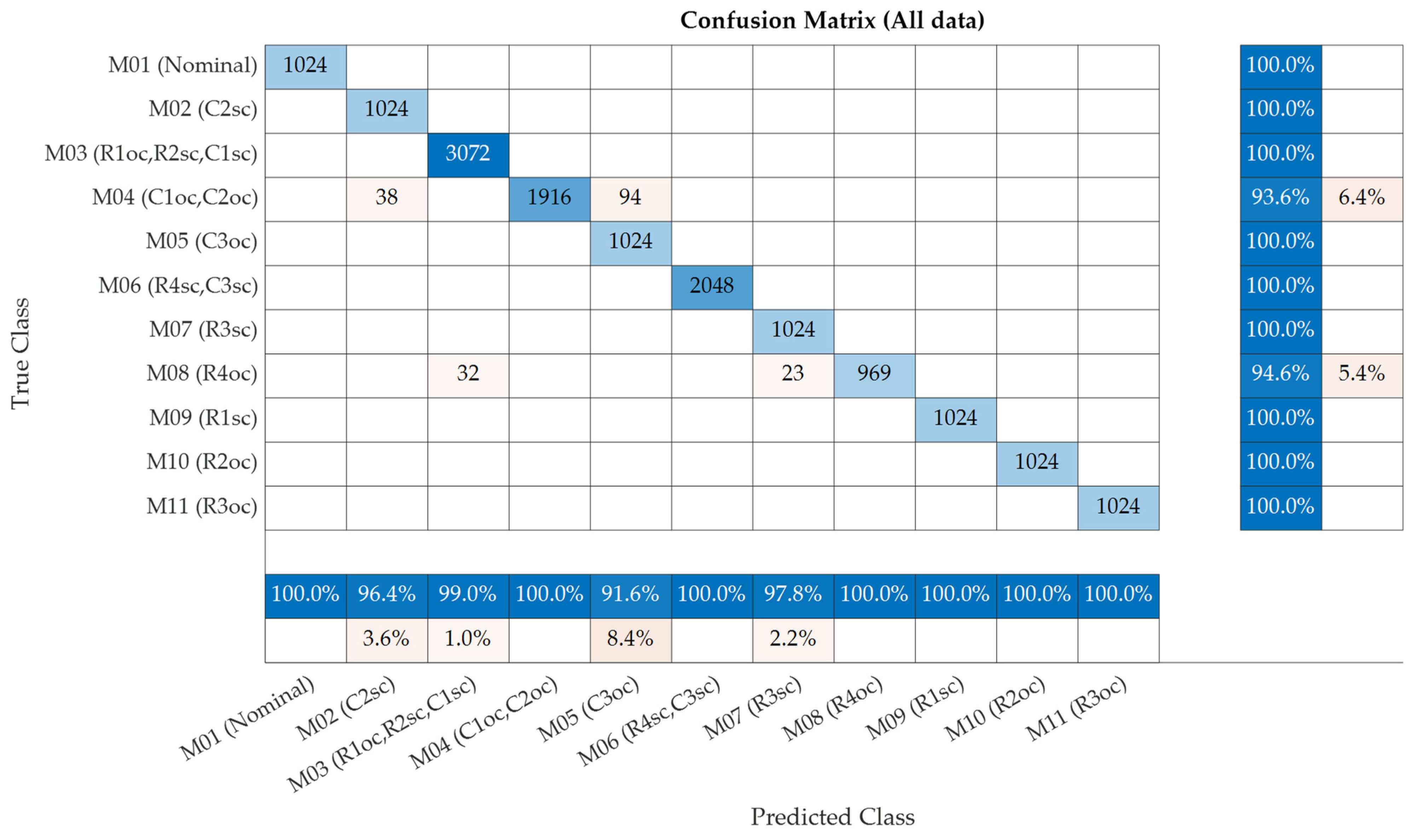
Figure 19 shows the results of the confusion matrix obtained in the case of a wider range of variation in the fault resistance, for the first CUT. As can be noted, the ANN was able to correctly diagnose most of the fault classes that may arise in the first CUT, as well as the nominal behavior. A similar analysis could be carried out with the second CUT.

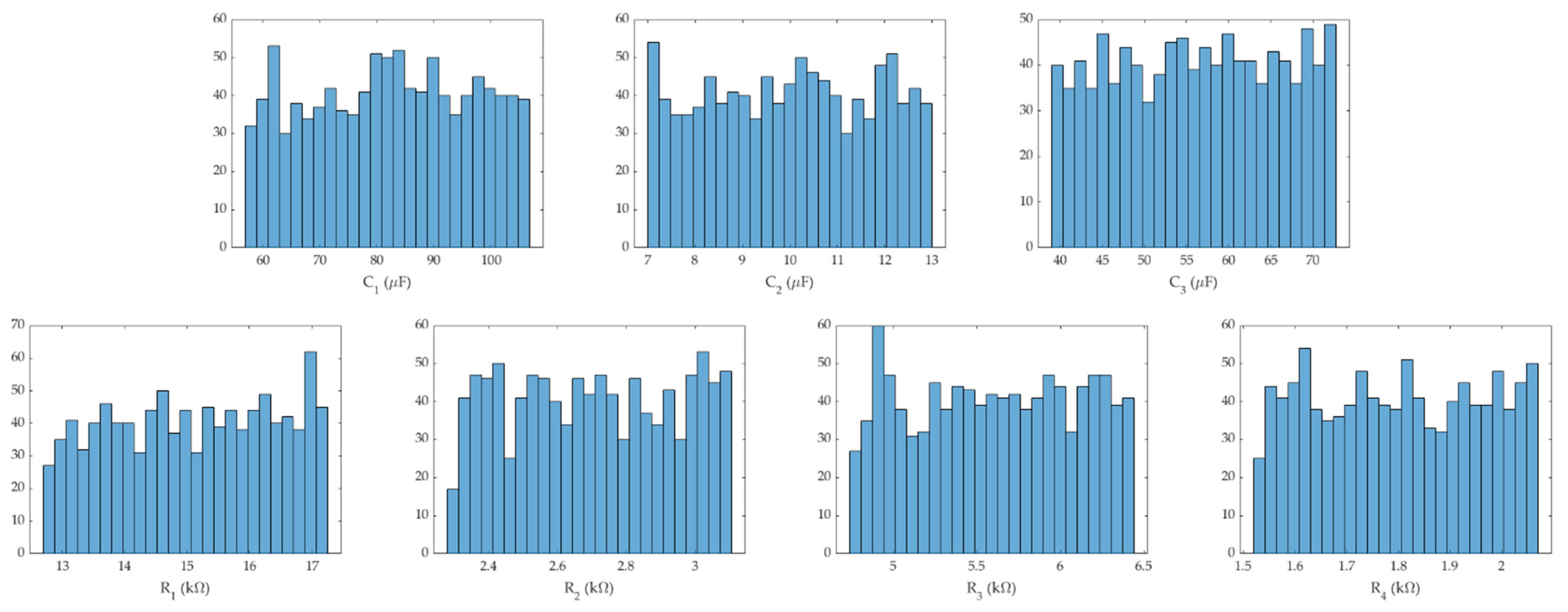
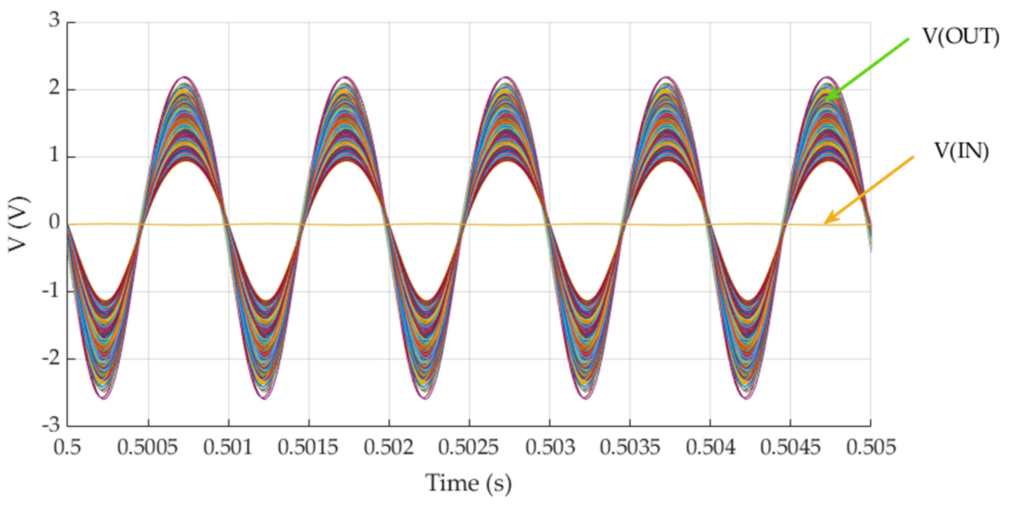
Specifically, it can be observed in Figure 19 that, when the first CUT works with the nominal values of the passive components, with their tolerances increased by 50%, the ANN predicted nominal behavior in all cases (100%), which is logical, since the BJT amplifier considered as the first CUT in this study was robust to variations in the tolerances of the passive components, so it was not greatly affected by the fact that these tolerances were increased by 50% with respect to the design values, as can be observed in Figure 20.

On the other hand, regarding the M₀₂ and M₀₃ classes, these were correctly diagnosed. In the case of M₀₄, there were some faults that were classified as M₀₂ and M₀₅ classes, which, at first, may seem like a detection failure by the ANN, but may have actually been caused by the fact that varying the resistance in series with C₁ and C₂ within the range of values analyzed (by setting 99.9% variation in the series fault resistance) can lead to a similar configuration from the point of view of the DC voltages of the transistor. In any case, 93.6% of the cases analyzed were correctly detected. Additionally, in the case of M₀₅, M₀₆, and M₀₇, 100% of the cases were detected correctly. Moreover, regarding the M₀₈ class the network predicted 94.6% of the faults. For the rest of the classes (M₀₉, M₁₀, and M₁₁), the ANN detected 100% of the faults.

Therefore, the ANN developed in this study could accurately predict the behavior of the first CUT when faced with variations in the fault resistance. Figure 21, Figure 22, Figure 23, Figure 24, Figure 25 and Figure 26 show the values predicted by the ANN versus the values of the fault resistance.

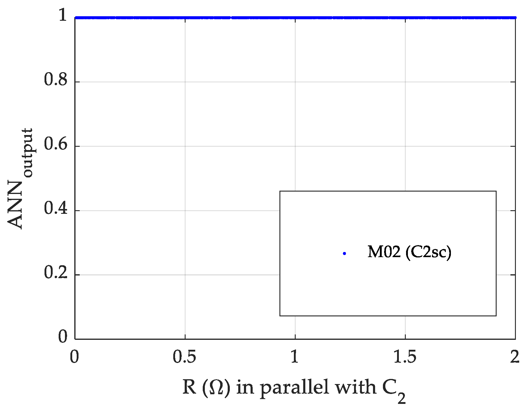
Figure 21 shows the values predicted by the ANN for the fault class M₀₂. It can be noted that the ANN detected all the faults in the circuit for the values of parallel resistance considered.

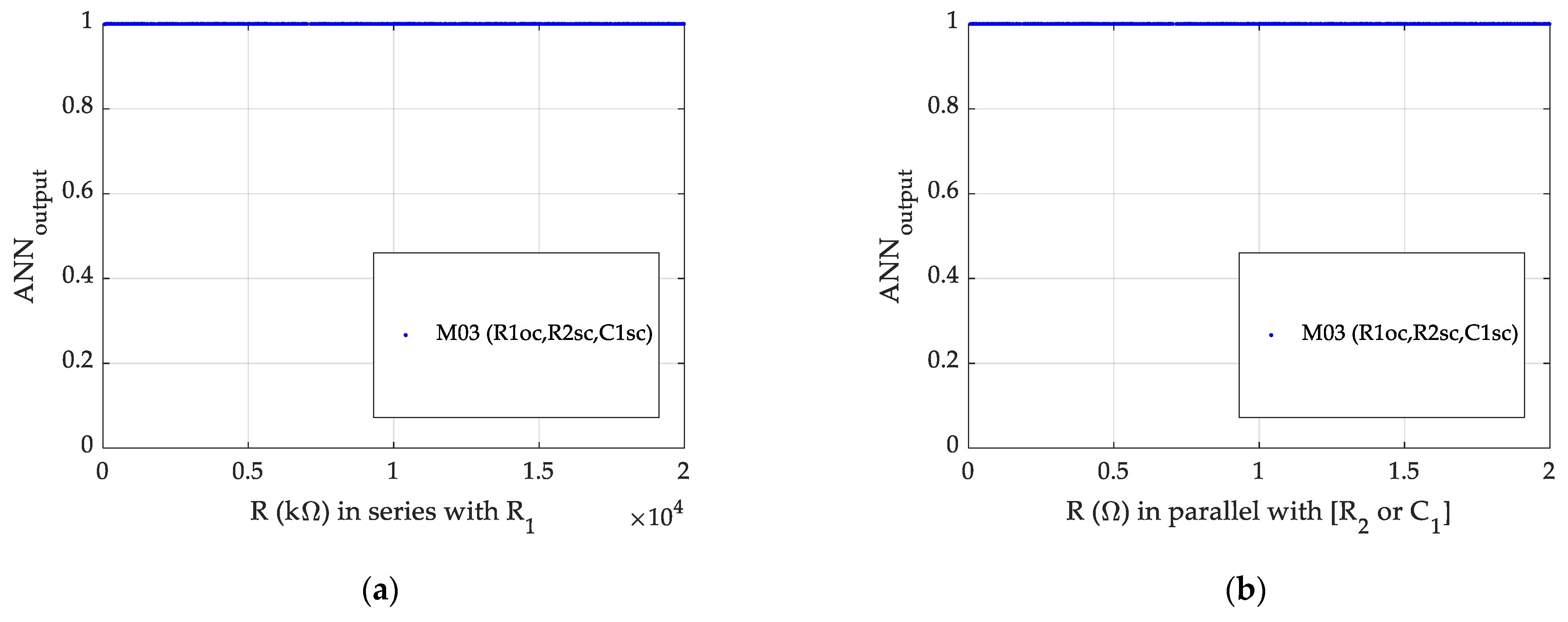
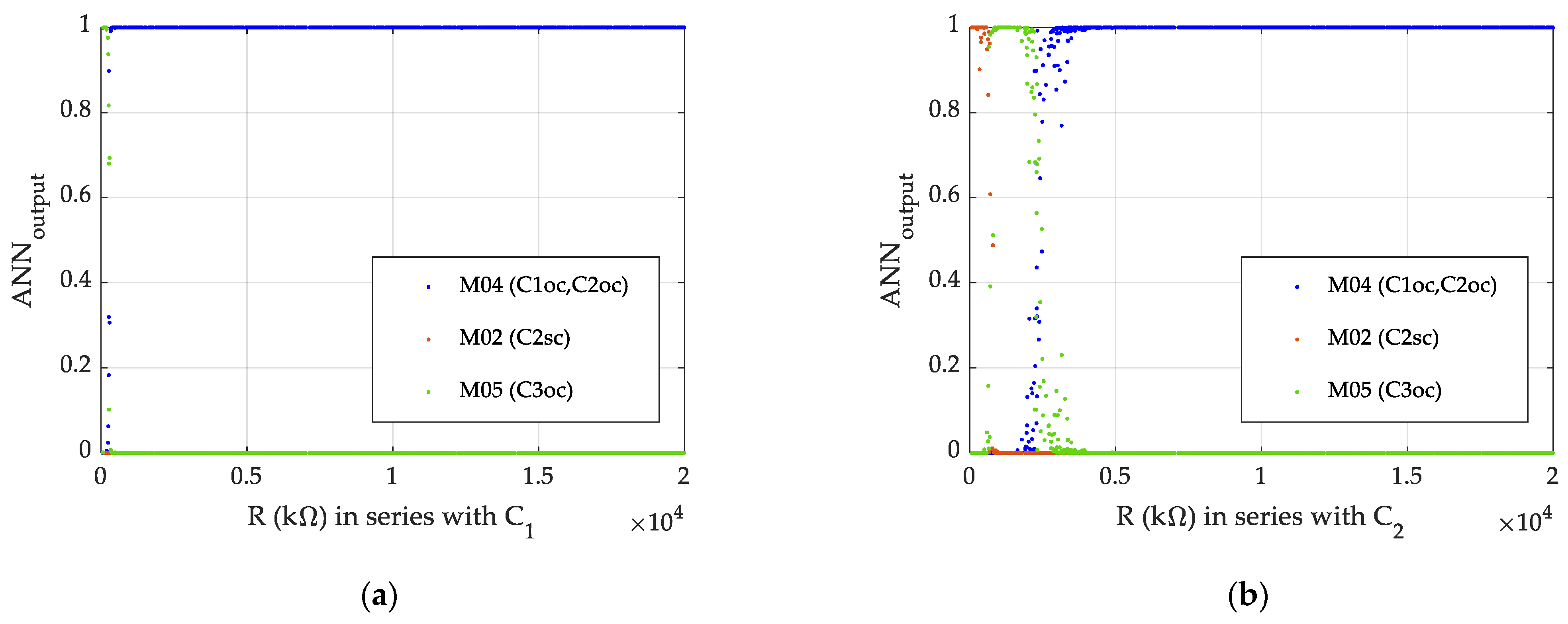
Figure 22 shows the values predicted by the ANN for fault class M₀₃. It can be noted that the ANN detected all the faults in the circuit for the values of serial and parallel resistances (R) considered. Likewise, Figure 23a shows that, in the case of C₁ for low values of resistance in series (R) with the faulty component, some of these situations could be detected as M₀₂{C_2sc} and M₀₅{C_3oc} since the values of the fault resistance in series with C₁ presented a minimum value of 64 kΩ, which was obtained in this study through Monte Carlo analysis with 1024 runs. The same behavior was obtained in the case of C₂, although for different thresholds of resistance (R), as can be observed in Figure 23b.

Figure 24a shows the values predicted by the ANN for the hard faults of class M₀₅ {C_3oc}, and Figure 24b shows those for the M₀₆ {R_4sc, C_3sc} and M₀₇ {R_3sc} fault classes. As can be observed, the ANN detected all the faults in the circuit.

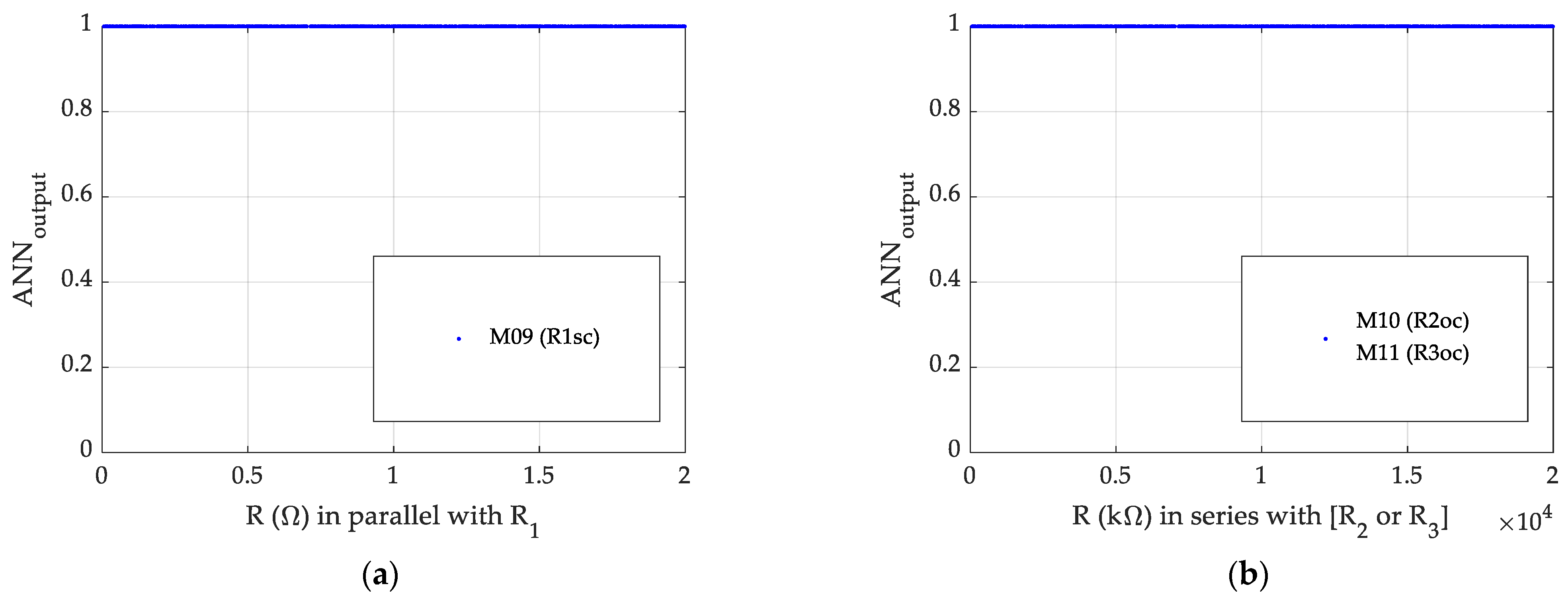
Figure 25 shows the results predicted by the ANN for the M₀₈ fault class (94.6% faults were detected). Finally, Figure 26 shows the results predicted for the remaining fault classes. As can be observed, 100% of fault data were correctly diagnosed in the case of R_1sc (M₀₉), R_2oc (M₁₀), and R_3oc (M₁₁).

5. Conclusions

In the present study, a pattern-recognition neural network with a hyperbolic tangent as the transfer function in the hidden layer, along with a softmax transfer function in the output layer, was used to diagnose individual hard faults in two CUTs. First, a single-stage small-signal BJT amplifier was studied, followed by a two-stage small-signal BJT amplifier. It was shown that the ANN was able to predict the hard faults accurately in both CUTs considered in this work.

It was shown that a pattern-recognition ANN such as the one considered in this study can be used to model hard faults in the CUTs by training the ANN with a reduced number of measurements that have been taken at accessible points of the circuit and by using only one hidden layer with a reduced number of neurons.

Moreover, in case of applying the neural network to situations different from those used to train the neural network, where these situations have been modeled by expanding the ranges of failure resistance, it was shown that the ANN developed had high precision in diagnosing the failures in the first CUT, and it was able to explain situations different from those used to train the ANN and to extract valuable information that may explain the behavior of the circuit.