
Bayesian Inference for Stochastic Cusp Catastrophe Model with Partially Observed Data


Abstract
:1. Introduction
- (1)
- If , for example , Equation (2) has three distinct real roots;
- (2)
- If , for example , Equation (2) has two distinct real roots with one of the two being a double root;
- (3)
- If , for example , Equation (2) has only one real root.
2. Inference from Partial Observations
2.1. Bayesian Data Augmentation
2.2. General Case
2.3. Hamiltonian Monte Carlo
| Algorithm 1: Implementation of Hamiltonian Monte Carlo. |
Start with a collection of samples with being the latest draw; Let be ; Sample a new initial momentum variable from ; Run the Leap Frog algorithm Algorithm 2 starting at for L steps with step-size to obtain proposed states and : Compute the acceptance ratio: Accept with following acceptance–rejection criterion: |
| Algorithm 2: Leap Frog algorithm. |
Take a half step forward in time to update the momentum variable while fixing position variable at t: Take a full step forward in time to update the position variable while fixing momentum variable computed at time from the previous step: Take the remaining half step in time to finish updating the momentum variable while fixing position variable at time : |
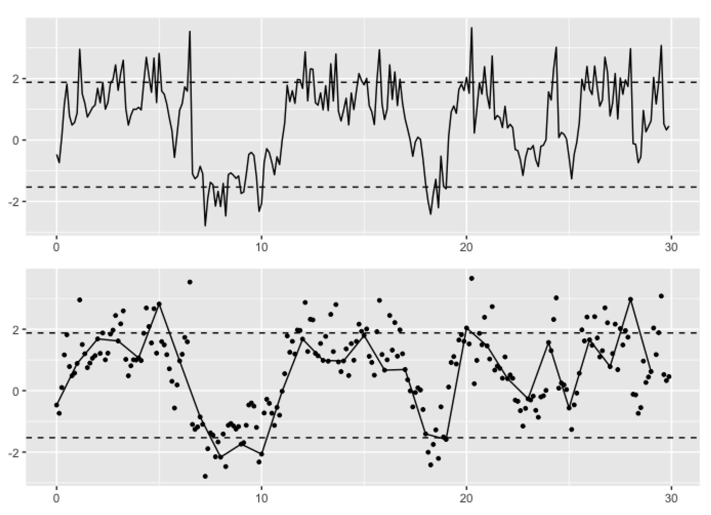
3. Simulation Study
3.1. Simulation Design
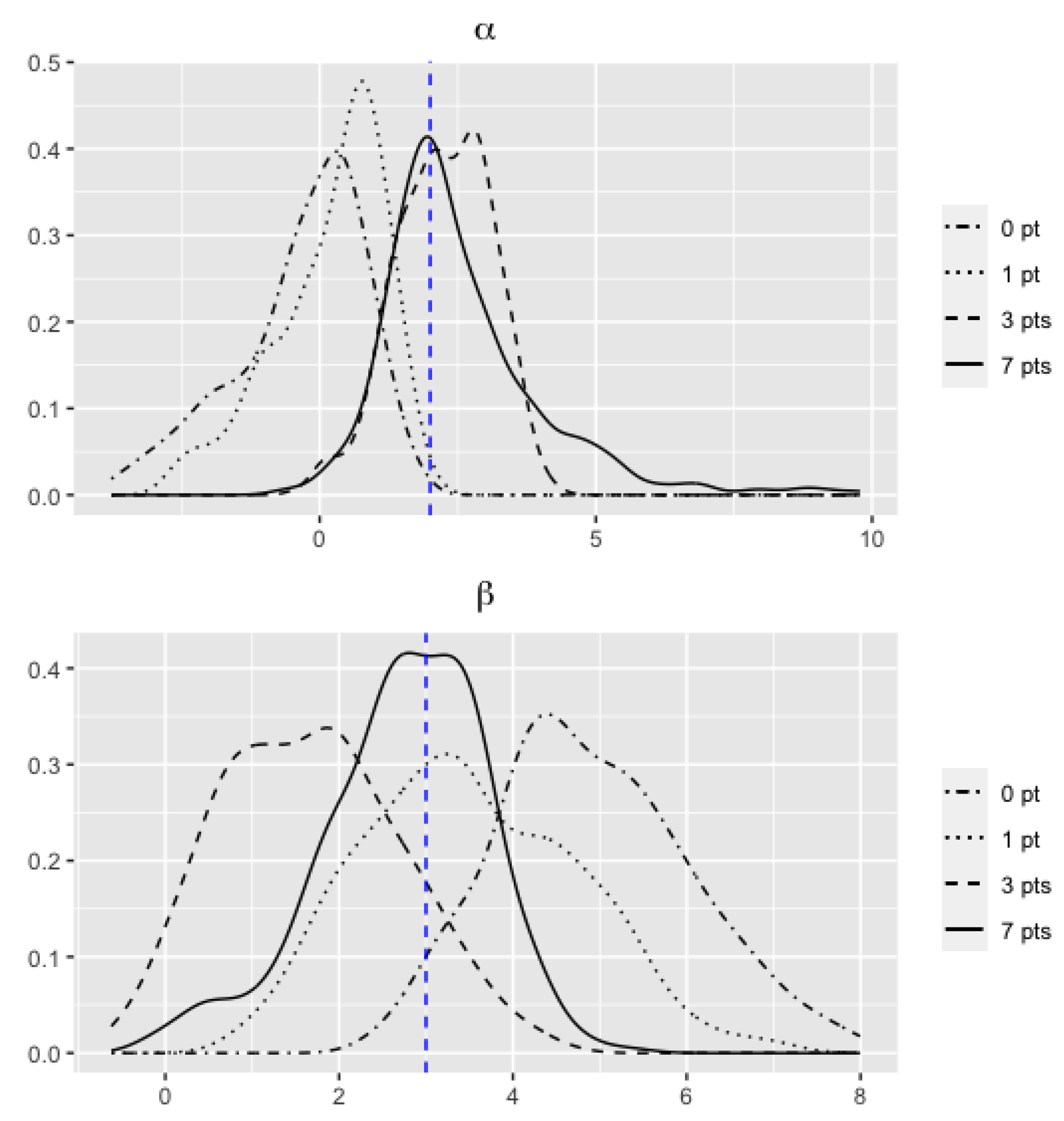
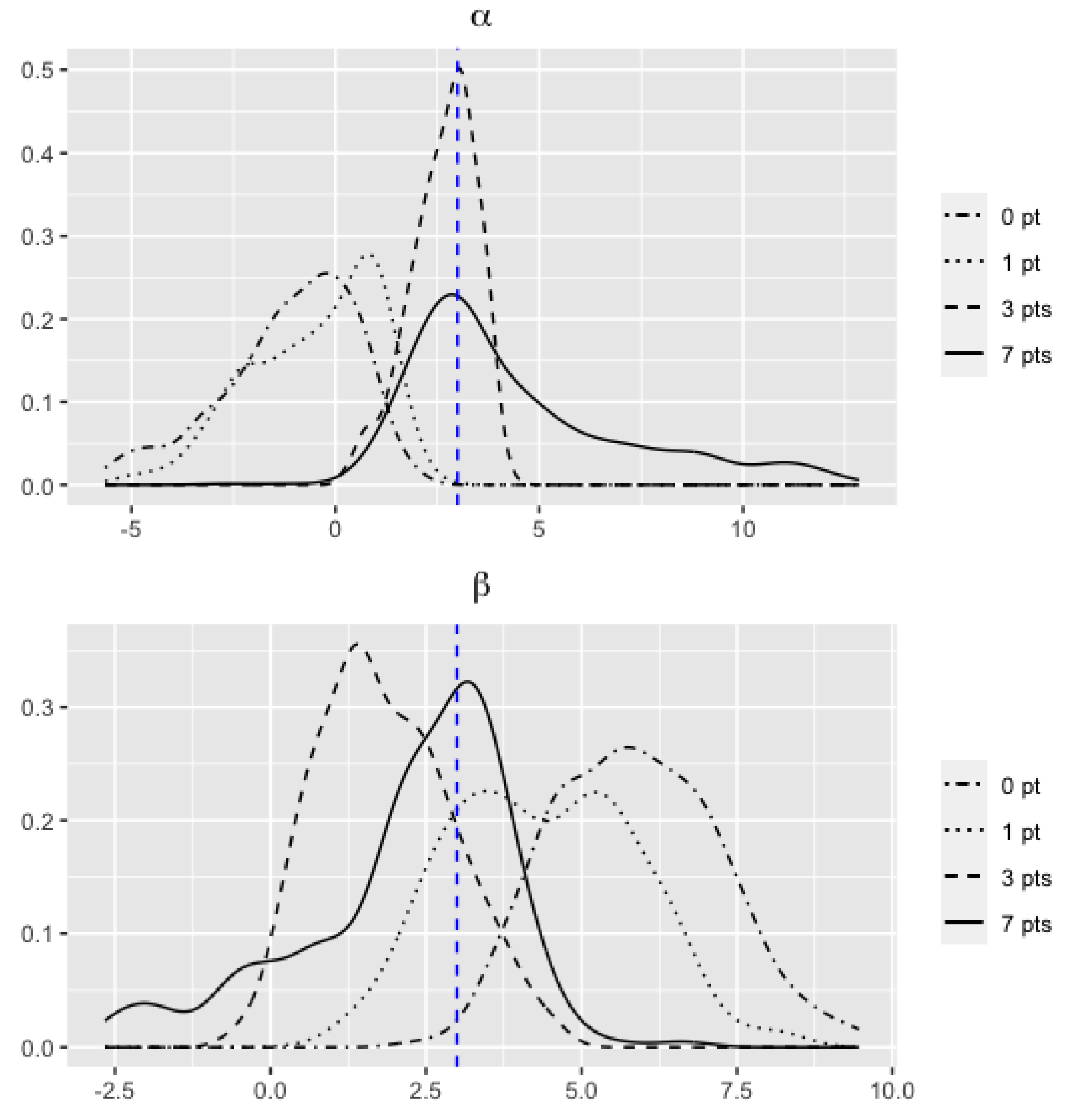
3.2. Results
4. Conclusions
Author Contributions
Funding
Institutional Review Board Statement
Informed Consent Statement
Data Availability Statement
Acknowledgments
Conflicts of Interest
References
- Thom, R.; Zeeman, E. Catastrophe theory: Its present state and future perspectives. In Dynamical Systems-Warwick; Springer: Berlin/Heidelberg, Germany, 1974; p. 366. [Google Scholar]
- Thom, R. Structural Stability and Morphogenesis; Benjamin-Addison-Wesley: New York, NY, USA, 1975. [Google Scholar]
- Thom, R.; Fowler, D.H. Structural Stability and Morphogenesis: An Outline of a General Theory of Models; W. A. Benjamin: New York, NY, USA, 1975. [Google Scholar]
- Cobb, L.; Ragade, R.K. Applications of Catastrophe Theory in the Behavioral and Life Sciences; Behavioral Science: New York, NY, USA, 1978; Volume 23, p. i. [Google Scholar]
- Cobb, L. Estimation Theory for the Cusp Catastrophe Model. In Proceedings of the American Statistical Association, Section on Survey Research Methods (March 1981); 1980; pp. 772–776. Available online: http://www.asasrms.org/Proceedings/papers/1980_162.pdf (accessed on 12 December 2021).
- Cobb, L.; Watson, B. Statistical catastrophe theory: An overview. Math. Model. 1980, 1, 311–317. [Google Scholar] [CrossRef] [Green Version]
- Cobb, L.; Zacks, S. Applications of catastrophe theory for statistical modeling in the biosciences. J. Am. Stat. Assoc. 1985, 80, 793–802. [Google Scholar] [CrossRef]
- Honerkamp, J. Stochastic Dynamical System: Concepts, Numerical Methods, Data Analysis; VCH Publishers: New York, NY, USA, 1994. [Google Scholar]
- Hartelman, A.I. Stochastic Catastrophe Theory; University of Amsterdam: Amsterdam, The Netherlands, 1997. [Google Scholar]
- Grasman, R.P.; van der Mass, H.L.; Wagenmakers, E. Fitting the cusp catastrophe in R: A cusp package primer. J. Stat. Softw. 2009, 32, 1–27. [Google Scholar] [CrossRef] [Green Version]
- Chen, D.G.; Gao, H.; Ji, C.; Chen, X. Stochastic cusp catastrophe model and its Bayesian computations. J. Appl. Stat. 2021, 1–20. [Google Scholar] [CrossRef]
- Melino, A. Estimation of continuous-time models in finance. In Advances in Econometrics Sixth World Congress; Sims, C.A., Ed.; Cambridge University Press: Cambridge, UK, 1996; Volume 2, pp. 313–351. [Google Scholar]
- Jones, C.S. Bayesian Estimation of Continuous-Time Finance Models; University of Rochester: New York, NY, USA, 1998. [Google Scholar]
- Ait-Sahalia, Y. Closed-form likelihood expansions for multivariate diffusions. Ann. Stat. 2008, 36, 906–937. [Google Scholar] [CrossRef]
- Neal, R.M. MCMC using Hamiltonian dynamics. Handb. Markov Chain. Monte Carlo 2011, 2, 2. [Google Scholar]
- Betancourt, M. A conceptual introduction to Hamiltonian Monte Carlo. arXiv 2017, arXiv:1701.02434. [Google Scholar]
- Iacus, S.M. Simulation and Inference for Stochastic Differential Equations: With R Examples; Springer Science & Business Media: Berlin/Heidelberg, Germany, 2009. [Google Scholar]
- Platen, E. An introduction to numerical methods for stochastic differential equations. Acta Numer. 1999, 8, 197–246. [Google Scholar] [CrossRef] [Green Version]
- Gelman, A.; Stern, H.S.; Carlin, J.B.; Dunson, D.B.; Vehtari, A.; Rubin, D.B. Bayesian Data Analysis; Chapman and Hall: London, UK; CRC: Boca Raton, FL, USA, 2013. [Google Scholar]


| Factors | Values |
|---|---|
| Parameters (, ) | (1,3), (2,3), (3,3) |
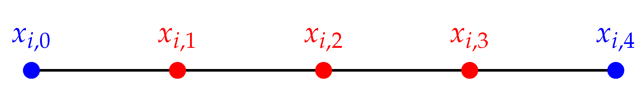
| Augmented points | 0, 1, 3, 7 |
| Notation | Description | Operation Level |
|---|---|---|
| , | posterior mode | per replication |
| , | standard error of posterior and | per replication |
| Mean , | mean of posterior modes | all replications |
| SE | standard error for and | all replications |
| ESE | mean standard error of posterior and | all replications |
| CP | coverage probability using 95% HCI among | all replications |
| Parameters | Aug. Pts | Mean | SE | ESE | Mean | SE | ESE | Both CP |
| 0 | 0.247 | 0.686 | 0.422 | 3.958 | 0.827 | 0.280 | 0.189 | |
| 1 | 0.441 | 0.582 | 0.898 | 2.699 | 0.841 | 0.474 | 0.613 | |
| 3 | 1.258 | 0.850 | 0.736 | 1.943 | 1.000 | 0.791 | 0.658 | |
| 7 | 1.149 | 0.761 | 0.771 | 2.897 | 0.701 | 0.767 | 0.902 | |
| 0 | −0.336 | 1.182 | 0.508 | 4.917 | 1.129 | 0.307 | 0.019 | |
| 1 | 0.198 | 1.015 | 0.749 | 3.513 | 1.237 | 0.530 | 0.249 | |
| 3 | 2.241 | 0.854 | 0.840 | 1.673 | 1.046 | 0.775 | 0.505 | |
| 7 | 2.559 | 1.487 | 1.475 | 2.731 | 0.955 | 1.121 | 0.812 | |
| 0 | −1.122 | 1.641 | 0.572 | 5.843 | 1.338 | 0.321 | 0.029 | |
| 1 | −0.494 | 1.582 | 0.862 | 4.370 | 1.488 | 0.550 | 0.024 | |
| 3 | 2.648 | 0.813 | 0.907 | 1.835 | 1.072 | 0.747 | 0.466 | |
| 7 | 4.435 | 2.722 | 1.864 | 2.194 | 1.687 | 1.353 | 0.715 | |
Publisher’s Note: MDPI stays neutral with regard to jurisdictional claims in published maps and institutional affiliations. |
© 2021 by the authors. Licensee MDPI, Basel, Switzerland. This article is an open access article distributed under the terms and conditions of the Creative Commons Attribution (CC BY) license (https://creativecommons.org/licenses/by/4.0/).
Share and Cite
Chen, D.-G.; Gao, H.; Ji, C. Bayesian Inference for Stochastic Cusp Catastrophe Model with Partially Observed Data. Mathematics 2021, 9, 3245. https://doi.org/10.3390/math9243245
Chen D-G, Gao H, Ji C. Bayesian Inference for Stochastic Cusp Catastrophe Model with Partially Observed Data. Mathematics. 2021; 9(24):3245. https://doi.org/10.3390/math9243245
Chicago/Turabian StyleChen, Ding-Geng, Haipeng Gao, and Chuanshu Ji. 2021. "Bayesian Inference for Stochastic Cusp Catastrophe Model with Partially Observed Data" Mathematics 9, no. 24: 3245. https://doi.org/10.3390/math9243245
APA StyleChen, D.-G., Gao, H., & Ji, C. (2021). Bayesian Inference for Stochastic Cusp Catastrophe Model with Partially Observed Data. Mathematics, 9(24), 3245. https://doi.org/10.3390/math9243245