Article

Green Supply Chain Management with Nash Bargaining Loss-Averse Reference Dependence

1
School of Business Administration, Hunan University of Finance and Economics, Changsha 410205, China
2
School of Business Administration, Research Center for Energy Economics, Henan Polytechnic University, Jiaozuo 454000, China
3
School of Business, Nanjing Audit University, Nanjing 211815, China
*
Author to whom correspondence should be addressed.
Mathematics 2021, 9(24), 3154; https://doi.org/10.3390/math9243154
Submission received: 20 October 2021 / Revised: 30 November 2021 / Accepted: 3 December 2021 / Published: 8 December 2021
(This article belongs to the Special Issue Supply Chain Management and Mathematical Logistics)

Abstract

:
This paper investigates a two-echelon green supply chain (GSC) with a single loss-averse manufacturer and a single loss-averse retailer. Since the Nash bargaining solution exactly characterizes endogenous power and the contribution of the GSC members, it is introduced as the loss-averse reference point for the GSC members. Based on this, a decision model of the two-echelon GSC with loss aversion is formulated. The optimal strategies of price and product green degree are derived in four scenarios: (a) the centralized decision scenario with rational GSC members, namely the CD scenario; (b) the decentralized decision scenario with rational GSC members, namely the DD scenario; (c) the decentralized decision scenario with the GSC members loss-averse, where the manufacturer’s share is below its own loss-averse reference point, namely the DD(∆mπm) scenario; (d) the decentralized decision scenario with the GSC members loss-averse, where the retailer’s share is below its own loss-averse reference point, namely the DD(∆rπr) scenario. Then, a comparative analysis of the optimal strategies and profits in these four scenarios is conducted, and the impacts of loss aversion and green efficiency coefficient of products (GECP) on the GSC are also performed. The results show that (i) GECP has a critical influence on the retail price and the wholesale price; (ii) the GSC with loss aversion provide green products with the lowest green degree; (iii) the retail price, the wholesale price and product green degree are decreasing monotonically with the loss aversion level of the GSC member without incurring loss; (iv) furthermore, the effect of the loss aversion level of the GSC member with incurring loss on the optimal strategies is related to GECP and the gap between the GSC members’ loss aversion levels.

1. Introduction

Global warming has critical effects on economies around the world, and the effects are continuously increasing. The increase of carbon dioxide emissions triggers the greenhouse effect, which is the most striking cause of global warming [1]. To cope with this problem, the Paris Agreement was signed by almost 200 countries in 2015, which aimed at controlling and mitigating the negative impacts incurred by climate change. In recent years, environmental protection has received increasingly attention, whose importance has been recognized increasingly by people. This has currently become a trend whereby the issues of pollution incurred by industrial development are addressed within the supply chain management (SCM) process [2]. Recent works have discussed such trends under green supply chain management (GSCM), and the concepts of environmental sustainability and sustainable development have been also introduced to GSCM [2,3,4]. Manufacturers and retailers in GSCM are incentivized to take into account green products while they make business decisions. Implementing GSCM for manufacturers as well as retailers is a win-win strategy [5,6,7].
To improve the efficiency in resources utilization and reduce the effect of producing on environment, numerous countries focus on establishing a green supply chain (GSC). Some countries not only strengthen the legislation and the supervision on the environmental protection, but also provide subsides to green enterprises [8,9,10,11,12]. In fact, GSC has received adequate attention from scientific circles with the exception of political cycles. Numerous previous works on GSC are limited to the various barriers about implementing GSC within different industries [13,14,15]. In recent years, numerous scholars have constructed GSC decision models based on game theory to analyze the decision rules for members, such as promoting cooperation [16,17,18,19,20]. The above works on GSC decision models considered the rational preferences of GSC members, namely, the GSC decisions were investigated based on the expected utility theory. Nevertheless, there exist some examples indicating that the decisions of GSC members are not always identical to the maximizing expected profit. For instance, in 2007, Langsha Group terminated the cooperation with Wal-Mart, because of suffering losses from the cooperation compared with direct selling. Another example is that in 2010 Xuzhou Wanji Trading of China aborted cooperation with Procter and Gamble after the former incurred losses. The above two examples indicate that the break-up occurs in the SCM since the loss-aversion behaviors of supply chain members are neglected by others. It is worthwhile noting that the United States of America withdraw from the Paris Agreement in 2020, since the Trump government argued that following the Paris Agreement cause the United States of America to lose nearly $3 trillion and decrease by more than 6.5 million industrial jobs and 3.1 million manufacturing jobs up to 2040 according to the Research Report of NERA Economic Consulting. Thus, a natural extension of GSC is to incorporate loss aversion of GSC members into GSCM.
The idea of loss aversion is introduced initially as the critical ingredient of prospect theory [21]. Value function is introduced by [22] to characterize the loss-aversion preferences of decision makers. According to [22], outcomes are framed as the gains (relative to a reference point) and the losses, and another feature of loss aversion is that losses loom is larger than gains. Inspired by [22], a simple and elegant utility function of loss aversion is introduced by [23]. In this version, a basic utility, a loss aversion coefficient and a reference point characterize the loss-aversion preference of decision makers: an outcome below the reference point are framed as a loss and its utility is from the basic utility by subtracting a disutility that is equal to this loss multiplied by the loss-aversion coefficient. Shalev’s version has been received widespread attention in the field of game theory [24,25,26,27]. In particular, the value function and its variants that characterizes the loss-aversion preference of decision makers has been applied to supply chain decisions [28,29,30,31,32]. Until recent years, the impacts of loss-aversion preferences on decisions have increasingly received attention from an increasing number of scholars in the SCM [33,34,35,36]. However, the extant works on supply chain involving loss aversion have not adequately taken into account the choice of loss-aversion reference points of supply chain members, but assumed that associated loss-aversion reference points are equal to zero or given exogenously. This leaves a critical issue that exogenous reference points cannot exactly characterize endogenous power and contributions such that loss-aversion perception is influenced.
To address the remaining issue, this paper adopted the Nash bargaining solution as the loss-aversion reference point of GSC members, which is a new perspective for investigating the impact of loss aversion on GSCM. In a two-person bargaining game, the Nash bargaining solution formulates how much one bargainer should be assigned from the total payoff, which highlights the fairness in distributing the total payoff. This means that the Nash bargaining solution balances fairness and efficiency in a two-person bargaining game [37,38,39,40,41]. Thus, Nash bargaining solution is regarded as the loss-aversion reference points of GSC members in this paper.
In this paper, a two-echelon GSC with a single loss-averse manufacturer and a single loss-averse retailer is considered. We investigated the impact of loss aversion of the manufacturer and the retailer on the GSC decisions by using the Nash bargaining game and Stackelberg game. This paper is organized as follows: in Section 2, the literature on the topic of GSCM and SCM with loss aversion is reviewed such that the contribution of this work is explained; in Section 3, decision models of the two-echelon GSC with rational preference and loss aversion are constructed, respectively; in Section 4, a comparative study is performed to explore the impact of the green efficiency coefficient of products (GECP) and loss aversion on GSC decisions; Section 5 is a numerical analysis; in Section 6, managerial insights are considered; in Section 7, conclusions are presented.

2. Literature Review

Many researchers have investigated GSCM, but the most relevant works on GSCM is the optimal strategy for product green degree. Ghosh and Shah [42] investigated the impact of supply chain structure on a product’s green degree, the wholesale price and the retail price. Swami and Shah [43] investigated the impact of green sensitivity and the greening cost on product green degree. Ghosh and Shah [44] investigated the impact of cost sharing contract on product green degree and prices, and argued that the products with a higher green degree can be manufactured if the cost sharing contract is implemented. Zhu and He [45] argued that price competition of retailers can improve product green degree. Yenipazarli [46] argued that investing much capital in green technology cannot ensure a higher product green degree, and the price sensitivity for consumers has a critical impact on manufacturer’s decision. Bai et al. [47] constructed a GSC game model with respect to product green degree, the retail price and sales effort in sensitive demand. They argued that the integrated GSC may not result in a high profit for each member. Ghosh et al. [48] argued that government regulations compel manufacturers to make products with higher green degree. Patra [49] investigated a smartphone supply chain and analyzed the impact of greening investment efficiency and product green degree on optimal preference. Gao and Zhang [50] studied the decisions of pricing, green degree and sales effort under uncertain demand, and found that the green degree coefficient significantly affects the pricing, green degree and sales effort, and it is positive. The above works on GSCM are limited to the GSC members’ rational preferences, which ignore the fact that rational preferences are not always able to describe adequately their behavior preferences, because they may be loss averse. However, few works concern the effect of loss aversion on product green degree.
On the other hand, the extant works on SCM with loss aversion focus on a traditional SCM, instead of GSCM. Numerous scholars investigated a supply chain with a loss-averse retailer. For example, Liu et al. [51] argued that a higher loss aversion leads to a lower order quantity. Lee et al. [52] considered the supply option problem when a loss-averse newsvendor has multiple options. Hu et al. [53] investigated the impact of retailer’s loss aversion on the three-echelon supply chain coordination. Zhang et al. [54] pointed out that retailer’s loss aversion decreases the required initial working capital. Xu et al. [55] argued that the retailer suffers from its own loss aversion if the optimal option purchase quantity is given. Additionally, Huang et al. [56] considered a supply chain with a loss-averse manufacturer. They proposed that the contract parameter depends on loss aversion and the manufacturer benefits from its own loss aversion in certain condition. Feng and Tan [57] also analyzed the decisions of the GSC with a loss-averse manufacturer and a risk-neutral retailer, and pointed out that a greening cost-sharing contract can improve the profits of the GSC members if the retailer shares an appropriate proportion with the loss-averse manufacturer. Although the work of [57] is very similar to this research, they only analyzed the impact of the manufacturer’s loss aversion and its loss-averse reference point is equal to the subgame perfect equilibrium partition in the Rubinstein alternating-offers bargaining game, which is a complex bargaining process. For the supply chain with loss-averse consumers, Yang and Xiao [58] constructed a two-period game to investigate the influence of consumers’ loss aversion on wholesale price. They proposed that the wholesale price increases with loss aversion in the first period game, but decreases with loss aversion in the second period game. Liu et al. [59] analyzed the price strategy in a dual-channel supply chain if consumers are loss averse. It is worthwhile noting that Du et al. [60] investigated the impact of manufacturer’s and retailer’s loss aversion on the optimal decision in SCM. They argued that the optimal order for the retailer with loss aversion is positively related to wholesale price, but negatively related to retail price. They also found that the manufacturer with loss aversion produces more than the manufacturer with risk neutrality. Moreover, some scholars considered newsvendor problems with loss aversion. Wang [31], Ma et al. [33] and Wu et al. [35] argued that newsvendors’ loss aversion decreases order quantity. Lee et al. [52] considered the supply option problem when a loss-averse newsvendor has multiple options. Xu et al. [61] argued that a higher loss aversion leads to a lower fill rate without shortage cost, while a higher loss aversion leads to a higher fill rate if the shortage cost is sufficient high. Almost all of above works on SCM with loss aversion assume that one member is loss averse and the reference point is given exogenously. However, the exogenous reference points of the supply chain members cannot characterize endogenous power and the contribution of them exactly. In contrast to above works, we examine the optimal strategies of the two-echelon GSC with a single loss-averse manufacturer and a single loss-averse retailer, where the Nash bargaining solution is regarded as the loss-aversion reference points to characterize the endogenous power and contribution of the GSC members.

3. Model Description

3.1. Prior Assumptions

A two-echelon green supply chain is considered, which consists of a single manufacturer and a single retailer. The manufacturer supplies green products to the retailer at a wholesale price w, and the retailer sells these green products to the consumers at a retail price p. When purchasing a green product, the consumers consider the retail price as well as the product green degree.
Some assumptions are shown as follows.
Assumption 1.
Demand function of the green products is impacted by the retail price as well as the product’s green degree, simultaneously. According to Liu et al. [62], and Dey and Saha [63], the demand function is assumed to be a linear one with respect to the retail price and the product’s green degree. Specifically, the demand function is q = a + τe − p, where a is the potential demand of the market on green products, e is the product green degree, τ is the consumer sensitivity to green improvements, p is the retail price of a unit of green product.
Assumption 2.
To improve the product’s green degree, the manufacturer should invest much capital in new technology. With reference to Ghosh and Shah [42] and Swami and Shah [43], the manufacturer’s greening cost is he2/2, where h is the cost coefficient of a unit of green degree.
Assumption 3.
All information with respect to the manufacturer as well as the retailer are common knowledge, i.e., complete and symmetrical.
Assumption 4.
Coefficient τ 2 / h consists of the consumer sensitivity to green improvements and the cost coefficient of a unit of green degree, which is defined as the green efficiency coefficient of products (GECP) [57].
From Assumptions 1 and 2, it follows that the manufacturer’s profit is:
π m = ( a + τ e p ) ( w c ) 1 2 h e 2 ,
the retailer’s profit is:
π r = ( a + τ e p ) ( p w ) ,
and the profit of the whole GSC is:
π s c = ( a + τ e p ) ( p c ) 1 2 h e 2
where c is the manufacturing cost of a unit of green product.

3.2. Model Development

3.2.1. The Models with Rational Green Supply Chain (GSC) Members

For facilitating our comparative analysis in the subsequent sections, two scenarios with rational GSC members are considered: centralized decision with rational GSC members (i.e., CD scenario) and decentralized decision with rational GSC members (DD scenario).
(1)
CD scenario
In the CD scenario, the two-echelon GSC is in the control of one decision maker, who has rational preference and aims at maximizing the profit of the whole GSC system. The Hessian matrix with respect to p and e is shown as follows:
( 2 τ τ h )
If 0 < τ 2 / h < 2 , then this matrix is a negatively definite one. This means that the function formulated by Equation (3) is a joint concave function with respect to p and e. Thus, in order to maximize the profit function formulated by Equation (3), we have:
e = τ ( a c ) 2 h τ 2
p = c + ( a c ) h 2 h τ 2
Substituting Equations (4) and (5) into Equation (3) yields:
π s c c = h ( a c ) 2 2 ( 2 h τ 2 )
(2)
DD scenario
In the DD scenario, the manufacturer and the retailer, who are rational, aim at seeking the maximum of their own profits respectively. A Stackelberg game model of the GSC are formulated, in which the manufacturer is the leader and determines the wholesale price as well as the product green degree, and the retailer is the follower and decides the retail price. Differentiating Equation (2) with respect to p yields:
p = ( a + w + τ e ) / 2
Substituting Equation (7) into Equation (1) yields:
π m ( p , e , w ) = ( a + τ e w ) ( w c ) 2 1 2 h e 2
The Hessian matrix with respect to w and e is shown as follows:
( 1 τ / 2 τ / 2 h )
If 0 < τ 2 / h < 4 , then this matrix is a negatively definite one. This implies that the manufacturer’s profit function formulated by Equation (8) is a joint concave function with respect to w and e. Thus, to maximize manufacturer’s profit, we have:
w D = c + 2 h ( a c ) 4 h τ 2
e D = τ ( a c ) 4 h τ 2
Substituting Equations (9) and (10) into Equation (7) yields:
p D = c + 3 h ( a c ) 4 h τ 2
Substituting Equations (9)–(11) into Equations (1)–(3) yields the profits of the manufacturer, the retailer and the whole supply chain system, respectively.
π m D = h ( a c ) 2 2 ( 4 h τ 2 )
π r D = h 2 ( a c ) 2 ( 4 h τ 2 ) 2
π s c D = h ( a c ) 2 ( 6 h τ 2 ) 2 ( 4 h τ 2 ) 2

3.2.2. The Models with Loss-Averse GSC Members

In the two-echelon GSC, both the manufacturer and the retailer are not completely rational, but have loss aversion when they suffer a loss. This means that they will be loss-averse when their profits are less than their own loss-averse reference point. Therefore, in this section, we develop a Stackelberg game model of the GSC with loss aversion. Firstly, by introducing Nash bargaining solution as the loss-averse reference point, we model the loss aversion of the GSC members. Secondly, according to the characteristics of profit structure of the two-echelon GSC and Nash bargaining solution, two scenarios are discussed. One is the DD(∆mπm) scenario, where only the manufacturer’s share is below his own loss-averse reference point, i.e., only the manufacturer suffers a loss. The other is the DD(∆rπr) scenario, where only the retailer’s share is below his own loss-averse reference point, i.e., only the retailer suffers a loss. Then, the optimal strategies of price and product green degree and profits are obtained.
(1)
Loss aversion with Nash bargaining reference point
For the GSC members with loss aversion, their utilities depend on their own realized benefit and the gap between their own benefit and loss-averse reference point. A linear loss-aversion form introduced by [23] is applied to formulating the utility of each GSC member as follows:
u i = { π i π i Δ i π i λ i ( Δ i π i ) π i < Δ i ,
or, equivalently,
u i = ( 1 + λ i ) π i λ i max { π i , Δ i }
where i = m, r denotes the manufacturer and the retailer. λi > 0 is the loss aversion coefficient of the GSC member i. πi is the realized material payoff of the GSC member i. ∆i is the loss-averse reference point of the GSC member i. Since the loss-averse reference point of each GSC member comes from the psychological game—Nash bargaining game for fairly distributing profit of the whole GSC, these reference points must satisfy the Pareto efficiency axiom, i.e., Δ m + Δ r = π s c .
Lemma 1.
The loss-averse reference points depend on the loss-aversion coefficients of the manufacturer as well as the retailer. Specifically, the loss-averse reference points of the manufacturer and the retailer are shown as follows:
Δ m = ( 1 + λ r ) π s c 2 + λ m + λ r ; Δ r = ( 1 + λ m ) π s c 2 + λ m + λ r .
The proof of Lemma 1 is shown in Appendix A.
Based on these loss-averse reference points Equation (16), we can obtain the manufacturer’s utility and the retailer’s utility by substituting Equation (16) into Equation (15). Then, DD(∆mπm) scenario and DD(∆rπr) scenario are considered, and the optimal strategies and profits of these two scenarios are obtained.
(2)
DD(∆mπm) scenario
In DD(∆mπm) scenario, both the manufacturer and the retailer are loss-averse, and only the manufacturer’s share is below his own loss-averse reference point. Thus, the manufacturer incurs a loss, which implies that the retailer does not incur loss even if he is loss averse. The utilities of the manufacturer and the retailer are shown, respectively:
u m = ( 1 + λ m ) π m λ m Δ m = ( 1 + λ m ) [ ( a + τ e p ) ( w c ) 1 2 h e 2 ] λ m ( 1 + λ r ) [ ( a + τ e p ) ( p c ) 1 2 h e 2 ] 2 + λ m + λ r
u r = π r = ( a + τ e p ) ( p w )
We construct a Stackelberg game model with the manufacturer as the leader, determining the wholesale price as well as product green degree, while the retailer is the follower, determining the retail price. Differentiating Equation (18) with respect to p yields:
p = ( a + w + τ e ) / 2
Substituting Equation (19) into Equation (17) yields:
u m = ( 1 + λ m ) [ a + τ e w 2 ( w c ) 1 2 h e 2 ] λ m ( 1 + λ r ) [ ( a + τ e w ) / 2 ) ( ( a + w + τ e ) / 2 c ) 1 2 h e 2 ] 2 + λ m + λ r
The Hessian matrix with respect to w and e is shown as follows:
( 1 λ m + λ m ( 1 + λ r ) 2 ( 2 + λ m + λ r ) ( 1 + λ m ) τ 2 ( 1 + λ m ) τ 2 ( 1 λ m ) h λ m ( 1 + λ r ) ( τ 2 / 2 h ) 2 + λ m + λ r )
If 0 < τ 2 / h < φ , where φ = 4 + 2 λ m ( 1 + λ r ) / [ ( 1 + λ m ) 2 + 1 + λ r ] , then this matrix is a negatively definite one. This implies that the manufacturer’s utility function formulated by Equation (20) is a joint concave function with respect to w and e. Thus, to maximize manufacturer’s utility, we have:
w D , Δ m = c + 2 h ( 1 + λ m ) ( 2 + λ m + λ r ) ( a c ) h [ 4 ( 1 + λ m ) 2 + 4 ( 1 + λ r ) + 2 λ m ( 1 + λ r ) ] [ ( 1 + λ m ) 2 + ( 1 + λ r ) ] τ 2
e D , Δ m = τ [ ( 1 + λ m ) 2 + ( 1 + λ r ) ] ( a c ) h [ 4 ( 1 + λ m ) 2 + 4 ( 1 + λ r ) + 2 λ m ( 1 + λ r ) ] [ ( 1 + λ m ) 2 + ( 1 + λ r ) ] τ 2
Substituting Equations (21) and (22) into Equation (19) yields:
p D , Δ m = c + h ( 3 λ m 2 + 2 λ m λ r + 8 λ m + 3 λ r + 6 ) ( a c ) h [ 4 ( 1 + λ m ) 2 + 4 ( 1 + λ r ) + 2 λ m ( 1 + λ r ) ] [ ( 1 + λ m ) 2 + ( 1 + λ r ) ] τ 2
Substituting Equations (21)–(23) into Equations (1)–(3) yields the profits of the manufacturer, the retailer and the whole supply chain system, respectively.
π m , D , Δ m = h [ ( 1 + λ m ) 2 + ( 1 + λ r ) ] { 4 h [ ( 1 + λ m ) 2 + ( 1 + λ r ) + λ m ( 1 + λ r ) ] [ ( 1 + λ m ) 2 + ( 1 + λ r ) ] τ 2 } ( a c ) 2 2 { h [ 4 ( 1 + λ m ) 2 + 4 ( 1 + λ r ) + 2 λ m ( 1 + λ r ) ] [ ( 1 + λ m ) 2 + ( 1 + λ r ) ] τ 2 } 2
π r , D , Δ m = h [ ( 1 + λ m ) 2 + ( 1 + λ r ) ] { 4 h [ ( 1 + λ m ) 2 + ( 1 + λ r ) + λ m ( 1 + λ r ) ] [ ( 1 + λ m ) 2 + ( 1 + λ r ) ] τ 2 } ( a c ) 2 2 { h [ 4 ( 1 + λ m ) 2 + 4 ( 1 + λ r ) + 2 λ m ( 1 + λ r ) ] [ ( 1 + λ m ) 2 + ( 1 + λ r ) ] τ 2 } 2
π s c , D , Δ m = h [ ( 1 + λ m ) 2 + ( 1 + λ r ) ] { h [ 5 ( 1 + λ m ) 2 + 5 ( 1 + λ r ) + 4 λ m ( 1 + λ r ) ] [ ( 1 + λ m ) 2 + ( 1 + λ r ) ] τ 2 } ( a c ) 2 2 { h [ 4 ( 1 + λ m ) 2 + 4 ( 1 + λ r ) + 2 λ m ( 1 + λ r ) ] [ ( 1 + λ m ) 2 + ( 1 + λ r ) ] τ 2 } 2
(3)
DD(∆rπr) scenario
In the DD(∆rπr) scenario, both the manufacturer and the retailer are loss-averse, and only the retailer’s share is below his own loss-averse reference point. Thus, the retailer incurs a loss, which implies that the manufacturer does not occur loss even if he is loss averse. The utilities of the manufacturer and the retailer are shown, respectively, as:
u m = π m ( p , e , w ) = ( a + τ e p ) ( w c ) 1 2 h e 2
u r = ( 1 + λ r ) π r λ r Δ r = ( 1 + λ m ) ( a + τ e p ) ( p w ) λ r ( 1 + λ m ) [ ( a + τ e p ) ( p c ) 1 2 h e 2 ] 2 + λ m + λ r
A Stackelberg game model is constructed, where the manufacturer as the leader determines the wholesale price as well as product green degree, while the retailer as the follower determines the retail price. Differentiating Equation (28) with respect to p yields:
p = ( 1 + λ r ) ( 2 + λ m + λ r ) ( a + τ e + w ) λ r ( 1 + λ m ) ( a + τ e + c ) 2 [ ( 1 + λ r ) 2 + 1 + λ m ]
Substituting Equation (29) into Equation (27) yields:
u m = ( a + τ e ( 1 + λ r ) ( 2 + λ m + λ r ) ( a + τ e + w ) λ r ( 1 + λ m ) ( a + τ e + c ) 2 [ ( 1 + λ r ) 2 + 1 + λ m ] ) ( w c ) 1 2 h e 2
The Hessian matrix with respect to w and e is shown as follows:
( 1 λ r ( 1 + λ m ) ( 1 + λ r ) 2 + 1 + λ m τ 2 τ 2 h )
If 0 < τ 2 / h < ϑ , where ϑ = 4 + 4 λ r ( 1 + λ m ) / [ ( 1 + λ r ) 2 + ( 1 + λ m ) ] , then this matrix is a negatively definite one. This implies that the manufacturer’s utility function formulated by Equation (30) is a joint concave function with respect to w and e. Thus, to maximize manufacturer’s utility, we have:
w D , Δ r = c + 2 h [ ( 1 + λ r ) 2 + ( 1 + λ m ) ] ( a c ) 4 h ( 1 + λ r ) ( 2 + λ m + λ r ) [ ( 1 + λ r ) 2 + ( 1 + λ m ) ] τ 2
e D , Δ r = τ [ ( 1 + λ r ) 2 + ( 1 + λ m ) ] ( a c ) 4 h ( 1 + λ r ) ( 2 + λ m + λ r ) [ ( 1 + λ r ) 2 + ( 1 + λ m ) ] τ 2
Substituting Equations (31) and (32) into Equation (29) yields:
p D , Δ r = c + 3 h ( 1 + λ r ) ( 2 + λ m + λ r ) ( a c ) 4 h ( 1 + λ r ) ( 2 + λ m + λ r ) [ ( 1 + λ r ) 2 + ( 1 + λ m ) ] τ 2
Substituting Equations (31)–(33) into Equations (1)–(3) yields the profits of the manufacturer, the retailer and the whole supply chain system, respectively:
π m , D , Δ r = h [ ( 1 + λ r ) 2 + ( 1 + λ m ) ] ( a c ) 2 2 { 4 h ( 1 + λ r ) ( 2 + λ m + λ r ) [ ( 1 + λ r ) 2 + ( 1 + λ m ) ] τ 2 }
π r , D , Δ r = h 2 ( 2 + λ m + λ r ) [ ( 1 + λ m ) 2 + ( 1 + λ r ) + 3 λ r ( 1 + λ m ) ] 2 ( a c ) 2 { 4 h ( 1 + λ r ) ( 2 + λ m + λ r ) [ ( 1 + λ r ) 2 + ( 1 + λ m ) ] τ 2 } 2
π s c , D , Δ r = h { 6 h ( 1 + λ r ) 2 ( 2 + λ m + λ r ) [ ( 1 + λ r ) 2 + ( 1 + λ m ) ] 2 τ 2 } ( a c ) 2 2 { 4 h ( 1 + λ r ) ( 2 + λ m + λ r ) [ ( 1 + λ r ) 2 + ( 1 + λ m ) ] τ 2 } 2

4. Analysis and Comparison Equilibriums in Four Scenarios

Here, a comparative analysis is performed to explore the impact of GECP and loss aversion of the manufacturer and the retailer on optimal strategies and profits of the GSC with loss aversion.
Theorem 1.
For casem ≥ πm, (i) p D , Δ m > p D > p if 0 < τ 2 / h < 1 , (ii) p D , Δ m = p D = p if τ 2 / h = 1 , (iii) p D , Δ m < p D < p if 1 < τ 2 / h < 2 . For caser ≥ πr, (I) p D > p D , Δ r > p if 0 < τ 2 / h < ψ , (II) p D > p D , Δ r = p if τ 2 / h = ψ , (III) p D > p > p D , Δ r if ψ < τ 2 / h < 1 , (IV) p D = p > p D , Δ r if τ 2 / h = 1 , (V) p > p D > p D , Δ r if 1 < τ 2 / h < 2 .
The proof of Theorem 1 is shown in Appendix A.
Remark 1.
Form ≥ πm, Theorem 1 (i) demonstrates that the highest retail price is in DD (∆m ≥ πm), followed by in DD, while the lowest one is in CD, when GECP is low (i.e., 0 < τ 2 / h < 1 ). If GECP is high (i.e., 1 < τ 2 / h < 2 ), a reversed conclusion is inferred, as shown Theorem 1 (iii). If GECP is moderate (i.e., τ 2 / h = 1 ), the retail prices are identical in three decision scenarios. Forr ≥ πr, if GECP is sufficiently low (i.e., 0 < τ 2 / h < ψ ), then the highest retail price is in DD, while the lowest one is in CD, as shown in Theorem 1 (I). If GECP is high (i.e., 1 < τ 2 / h < 2 ), then the highest retail price is in CD, while the lowest one is in DD(r ≥ πr), as shown in Theorem 1(V). If GECP is low (i.e., ψ < τ 2 / h < 1 ), the highest retail price is in DD, while the lowest one is in DD(r ≥ πr), as shown in Theorem 1 (III). In addition, the conclusion that the retail price in DD is higher than that in CD, as shown in Theorem 1 (i), (I) and (II), is identical to the traditional supply chain, since lower GECP cannot lead to a significantly increase in market demand. The conclusion that the retail price in CD is higher than that in DD is reverse to the traditional supply chain, as shown in Theorem 1 (iii) and (V), since higher GECP leads to a higher awareness of consumers environmental protection such that consumers purchase green products, which also results in increasing market demand dramatically.
Proposition 1.
For casem ≥ πm,
(i) 
when 0 < τ 2 / h < 1 , d p D , Δ m d λ m > 0 if λ m < λ r + 2 and d p D , Δ m d λ m < 0 otherwise.
(ii) 
when 1 < τ 2 / h < φ , d p D , Δ m d λ m < 0 if λ m < λ r + 2 and d p D , Δ m d λ m > 0 otherwise.
(iii) 
d p D , Δ m d λ r > 0 if 0 < τ 2 / h < 1 and d p D , Δ m d λ r < 0 otherwise.
For caser ≥ πr,
(I) 
d p D , Δ r d λ m < 0 .
(II) 
d p D , Δ r d λ r < 0 if λ r < λ m + 2 and d w D , Δ r d λ r > 0 otherwise.
The proof of Proposition 1 is shown in Appendix A.
Remark 2.
Proposition 1 shows that for the casem ≥ πm GECP has a critical impact on the changes of retail price with the levels of loss aversion for the manufacturer and the retailer. When GECP is low, for λ m ( 0 , λ r + 2 ) ( λ m ( λ r + 2 , + ) ), the retail price increases (decreases) with the manufacturer’s level of loss aversion, while the retail price increases with the retailer’s level of loss aversion, as described in Proposition 1 (i) and (iii). When GECP is high, for λ m ( 0 , λ r + 2 ) ( λ m ( λ r + 2 , + ) ), the retail price decreases (increases) with the manufacturer’s level of loss aversion, as described in Proposition 1 (ii). while for the caser ≥ πr GECP has no effect on the changes of retail price with the levels of loss aversion for the manufacturer and the retailer. The retail price decreases with the manufacturer’s level of loss aversion, as described in Proposition 1 (I). The retail price decreases with the retailer’s level of loss aversion for λ r < λ m + 2 ; otherwise, it increases with the retailer’s level of loss aversion, as described in Proposition 1 (II). In addition, sincem ≥ πm implies that the retailer does not occurs loss, it follows from Proposition 1 that the retail price is increasing (decreasing) monotonically with the levels of loss aversion of the member without loss if GECP is low (high). On the other hand, sincer ≥ πr implies that the manufacturer does not occurs loss, according to Proposition 1, the retail price is decreasing monotonically with the levels of loss aversion of the member without loss.
Theorem 2.
For casem ≥ πm, (i) w D , Δ m > w D if 0 < τ 2 / h < 2 , (ii) w D , Δ m = w D if τ 2 / h = 2 , (iii) w D , Δ m < w D if 2 < τ 2 / h < 4 . For caser ≥ πr, w D , Δ r < w D .
The proof of Theorem 2 is shown in Appendix A.
Remark 3.
Theorem 2 indicates that GECP has an important impact on wholesale price. For case ∆m ≥ πm (i.e., a loss for the retailer with loss aversion has no occurs), Theorem 1(i) demonstrates that the wholesale price in DD(∆m ≥ πm) is higher than that in DD if GECP is low (i.e., 0 < τ 2 / h < 2 ). Theorem 1(iii) demonstrates that the wholesale price in DD(∆m ≥ πm) is less than that in DD if GECP is high (i.e., 2 < τ 2 / h < 4 ). Theorem 1(ii) demonstrates that the wholesale price in DD(∆m ≥ πm) is identical to that in DD if GECP is moderate (i.e., τ 2 / h = 2 ). For case ∆r ≥ πr (i.e., a loss for the manufacturer with loss aversion has no occurs), Theorem 2 demonstrates that the wholesale price in DD(∆r ≥ πr) is less than that in DD regardless of GECP.
Proposition 2.
For casem ≥ πm,
(i) 
when 0 < τ 2 / h < 2 , d w D , Δ m d λ m > 0 if λ m < λ r + 2 and d w D , Δ m d λ m < 0 otherwise.
(ii) 
when 2 < τ 2 / h < φ , d w D , Δ m d λ m < 0 if λ m < λ r + 2 and d w D , Δ m d λ m > 0 otherwise.
(iii) 
d w D , Δ m d λ r > 0 if 0 < τ 2 / h < 2 and d w D , Δ m d λ r < 0 otherwise.
For caser ≥ πr,
(I) d w D , Δ r d λ m < 0 . (II) d w D , Δ r d λ r < 0 if λ r < λ m + 2 and d w D , Δ r d λ r > 0 otherwise.
The proof of Proposition 2 is shown in Appendix A.
Remark 4.
Proposition 2 shows that for the casem ≥ πm GECP has a critical impact on the changes of wholesale price with the levels of loss aversion for the manufacturer and the retailer. When GECP is low, for λ m ( 0 , λ r + 2 ) ( λ m ( λ r + 2 , + ) ), the wholesale price increases (decreases) with the manufacturer’s level of loss aversion, while it increases with the retailer’s level of loss aversion, as described in Proposition 2 (i) and (iii). When GECP is high, for λ m ( 0 , λ r + 2 ) ( λ m ( λ r + 2 , + ) ), the wholesale price decreases (increases) with the manufacturer’s level of loss aversion, as described in Proposition 2 (ii) while for the case ∆r ≥ πr GECP has no effect on the changes of wholesale price with the levels of loss aversion for the manufacturer and the retailer. The wholesale price decreases with the manufacturer’s level of loss aversion, as described in Proposition 2 (I). The wholesale price decreases with the retailer’s level of loss aversion for λ r < λ m + 2 ; otherwise, it increases with the retailer’s level of loss aversion, as described in Proposition 2 (II). In addition, since ∆m ≥ πm implies that the retailer does not occurs loss, it follows from Proposition 2 that the wholesale price is increasing (decreasing) monotonically with the levels of loss aversion of the member without loss if GECP is low (high). On the other hand, since ∆r ≥ πr implies that the manufacturer does not occurs loss, according to Proposition 2, the wholesale price is decreasing monotonically with the levels of loss aversion of the member without loss.
Theorem 3.
For casem ≥ πm, e D , Δ m < e D < e . For caser ≥ πr, e D , Δ r < e D < e .
The proof of Theorem 3 is shown in Appendix A.
Remark 5.
From Theorem 3, it follows that the green degree is the highest in CD, followed by in DD, while it is the lowest in DD(m ≥ πm) or DD(r ≥ πr). This means that members with loss aversion are reluctant to engage in producing and selling green products such that product green degree is further decreased in DD(m ≥ πm) or DD(r ≥ πr).
Proposition 3.
For casem ≥ πm,
(i) d e D , Δ m d λ m < 0 if λ m < λ r + 2 and d e D , Δ m d λ m > 0 otherwise. (ii) d e D , Δ m d λ r < 0 .
For caser ≥ πr,
(I) d e D , Δ r d λ m < 0 .(II) d e D , Δ r d λ r > 0 if λ r < λ m + 2 and d e D , Δ r d λ r < 0 otherwise.
The proof of Proposition 3 is shown in Appendix A.
Remark 6.
For casem ≥ πm, Proposition 3 (i) shows that the product green degree decreases with the manufacturer’s level of loss aversion if λ m ( 0 , λ r + 2 ) ; otherwise, it increases with the manufacturer’s level of loss aversion. Proposition 3 (ii) shows that the product green degree decreases with the retailer’s level of loss aversion. For caser ≥ πr, Proposition 3 (I) shows that the product green degree decreases with the manufacturer’s level of loss aversion. Proposition 3 (II) shows that the product green degree increases with the retailer’s level of loss aversion if λ r < λ m + 2 ; otherwise, it decreases with the retailer’s level of loss aversion. In addition, sincem ≥ πm implies that the retailer does not occurs loss andr ≥ πr implies that the manufacturer does not incur loss, it follows from Proposition 3 that product green degree is decreasing monotonically with the levels of loss aversion of the member without loss.
Theorem 4.
For casem ≥ πm, π m , D , Δ m < π m D , π r , D , Δ m < π r D , π s c , D , Δ m < π s c D < π s c ( p , e ) . For caser ≥ πr, π m , D , Δ r < π m D , π s c , D , Δ r < π s c D < π s c ( p , e ) , for the retailer’s profit, (i) π r , D , Δ r > π r D if 0 < τ 2 / h < t , (ii) π r , D , Δ r = π r D if τ 2 / h = t , (iii) π r , D , Δ r < π r D if t < τ 2 / h < 4 .
The proof of Theorem 4 is shown in Appendix A.
Remark 7.
Form ≥ πm (i.e., a loss for the retailer with loss aversion has no occurs), the profits of the manufacturer and the retailer in DD(m ≥ πm) are less than that in DD. It implies that the manufacturer as well as the retailer are hurt by loss-averse preferences of members. On the other hand, the profit of the whole supply chain in CD is higher than that in DD, while the latter is higher than that in DD(m ≥ πm). Maximizing the profits of members leads to the decrease of the profit of the whole channel. Furthermore, once the manufacturer incurs loss, its loss-averse preference causes it to pay more attention to loss than gain, which further decreases the profit of the whole channel. Forr ≥ πr (i.e., a loss for the manufacturer with loss aversion has no consequence), the conclusions for the manufacturer and the whole supply chain are identical to the casem ≥ πm. For retailer’s profit, the gap between the profit of the loss-averse retailer and the profit of the rational retailer depends on GECP. If GECP is low (high), then the former is higher (less) than the latter.
Proposition 4.
For casem ≥ πm,
(i) d π m , D , Δ m d λ m < 0 if λ m < λ r + 2 and d π m , D , Δ m d λ m > 0 otherwise. (ii) d π m , D , Δ m d λ r < 0 . (iii) d π r , D , Δ m d λ m < 0 if λ m < λ r + 2 and d π r , D , Δ m d λ m > 0 otherwise. (iv) d π r , D , Δ m d λ r < 0 .
For caser ≥ πr,
(I) d π m , D , Δ r d λ m < 0 . (II) d π m , D , Δ r d λ r < 0 if λ r < λ m + 2 and d π m , D , Δ r d λ r > 0 otherwise.
(III) d π r , D , Δ r d λ m < 0 if 0 < τ 2 / h < θ ; d π r , D , Δ r d λ m > 0 if θ < τ 2 / h < ϑ .
(IV) when 0 < τ 2 / h < θ , d π r , D , Δ r d λ r > 0 if λ r < λ m + 2 and d π r , D , Δ r d λ r < 0 otherwise.
(V) when θ < τ 2 / h < ϑ , d π r , D , Δ r d λ r < 0 if λ r < λ m + 2 and d π r , D , Δ r d λ r > 0 otherwise.
where θ = 4 ( 1 + λ r ) ( 2 + λ m + λ r ) 3 λ m λ r + 2 λ r 2 + 2 λ m + 7 λ r + 4 and ϑ = 4 + 4 λ r ( 1 + λ m ) ( 1 + λ r ) 2 + 1 + λ m .
The proof of Proposition 4 is shown in Appendix A.
Remark 8.
For case m ≥ πm, the profits of the manufacturer and the retailer decrease with the levels of loss aversion for the manufacturer if λ m < λ r + 2 ; otherwise, the profits of the manufacturer and the retailer increase with the levels of loss aversion for the manufacturer while the profits of the manufacturer and the retailer decrease with the levels of loss aversion for the retailer. For caser ≥ πr, the manufacturer’s profit decreases with its own levels of loss aversion, while it also decreases with the retailer’s levels of loss aversion if λ r < λ m + 2 , and it increases with the retailer’s levels of loss aversion if λ r > λ m + 2 . It is worthwhile noting that GECP has a critical impact on the changes of retailer’s profit with the levels of loss aversion for the manufacturer and the retailer. When GECP is low, the retailer’s profit decreases with the manufacturer’s levels of loss aversion, while it increases with its own levels of loss aversion if λ r < λ m + 2 ; otherwise, it decreases with its own levels of loss aversion. When GECP is high, the retailer’s profit increases with the manufacturer’s levels of loss aversion, while it decreases with its own levels of loss aversion if λ r < λ m + 2 ; otherwise, it increases with its own levels of loss aversion.

5. Numerical Simulation

Signify, as a global lighting leader, occupies a leading position in the field of traditional lighting, light-emitting diodes (LEDs) and intelligent interconnected lighting. The global sales of Signify in 2020 were 6.5 billion €, of which the sales of LEDs were 70% of the total sales. However, with the rise in consumers’ environmental awareness, Signify has had to manufacture green LEDs (such as 3D printing downlights). For example, Signify adopts 100% recyclable polycarbonate materials and limits the number of screws and parts to reduce the difficulty of recycling in the production process of LEDs. In addition, Signify directly adopts colored materials to reduce additional coloring or post-treatment in the production process of LEDs. These reduce its carbon footprint by 75%. However, investing much capital in green technology will lead to a decrease of profits of Signify in the near future such that it prefers to minimize losses (relative to some reference point) rather than maximize gains. To investigate the effects of GECP and loss aversion on decision variables (i.e., product green degree, wholesale price and retail price) and profits, let the potential demand of the market on LEDs a = 120 and the manufacturing cost of a unit of LED c = 20 [64]. Here, Signify plays the role of the manufacturer.
To show the effects of GECP on decision variables, members’ profits and the overall profit, let λm = 1 and λr = 2, as described in Figure 1 and Figure 2. Figure 1 show the changes of decision variables with GECP, while Figure 2 shows the changes of members’ profits and the overall profit with GECP.
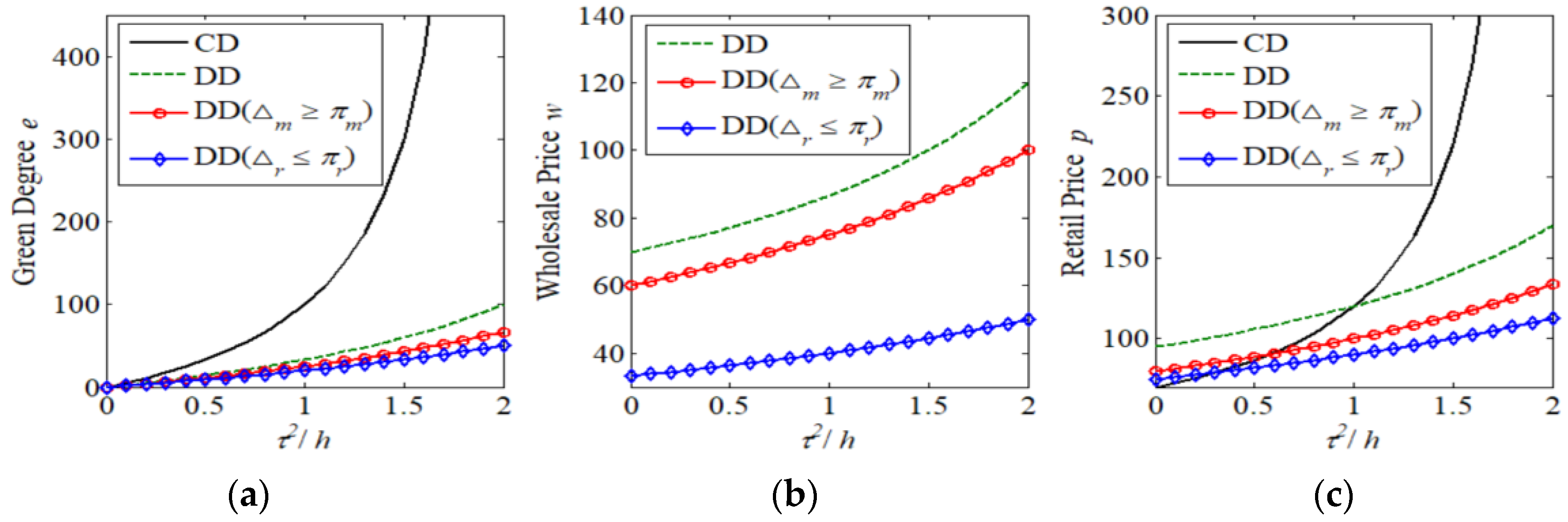
The effects of GECP on green degree, wholesale price and retail price are shown in Figure 1a–c, respectively. In Figure 1a, product green degree in four decision scenarios increase with GEPC. Product green degree in CD is the highest. After product green degree in CD, product green degree in DD is the second highest, followed by product green degree in DD(∆mπm), and in DD(∆rπr) is the lowest. In Figure 1b, the wholesale price in three decision scenarios (i.e., DD, DD(∆mπm) and DD(∆rπr)) increase with GEPC. The wholesale price in DD is the highest, followed by the wholesale price in DD(∆mπm), it in DD(∆rπr) is the lowest. In Figure 1c, the retail price in four decision scenarios increase with GEPC. GEPC has important impacts on the retail price in four decision scenarios. If GEPC is sufficiently low, then the highest retail price is in DD, while the lowest retail price is in CD. If GEPC is low, then the highest retail price is also in DD, while the lowest retail price is in DD(∆rπr). If GEPC is high, then the highest retail price is in CD, while the lowest retail price is in DD(∆rπr). In addition, in Figure 1c, the retail price in DD(∆mπm) is higher than the retail price in DD(∆rπr) regardless of GEPC. From Figure 1a–c), it follows that the loss-averse preferences of members decrease product green degree, the wholesale price and the retail price.
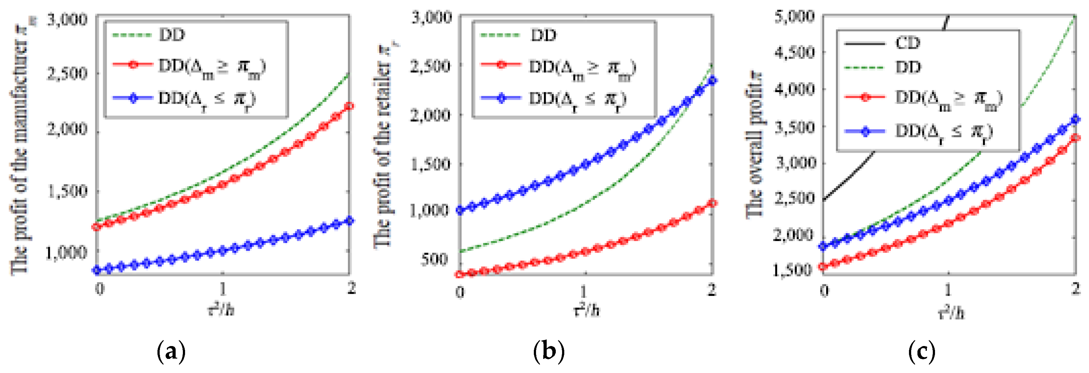
The impacts of GECP on the profits of Signify, retailer and the supply chain system are shown in Figure 2a–c, respectively. Figure 2a shows the changes of Signify’s profit with GEPC. In Figure 2a, Signify’s profit in three decision scenarios (i.e., DD, DD(∆mπm) and DD(∆rπr)) increases with GEPC. Signify’s profit in DD is the highest, followed by Signify’s profit in DD(∆rπr), and in DD(∆mπm) it is the lowest. Figure 2b shows the changes of the retailer’s profit with GEPC. If GEPC is sufficiently high, then the highest profit of the retailer is in DD, while the lowest profit of the retailer is in DD(∆mπm); otherwise, the highest profit of the retailer is in DD(∆rπr), while the lowest profit of the retailer is in DD(∆mπm). In Figure 2c, the overall profit in four decision scenarios increase with GEPC. The overall profit in CD is the highest. After the overall profit in CD, the overall profit in DD is the second highest, followed by the overall profit in DD(∆rπr), and in DD(∆mπm) it is the lowest. From Figure 2a–c, it follows that the loss-averse preferences of members decrease the profits of the members and the overall profit, and that the profit of a member incurring loss is higher than its profit without incurring loss.
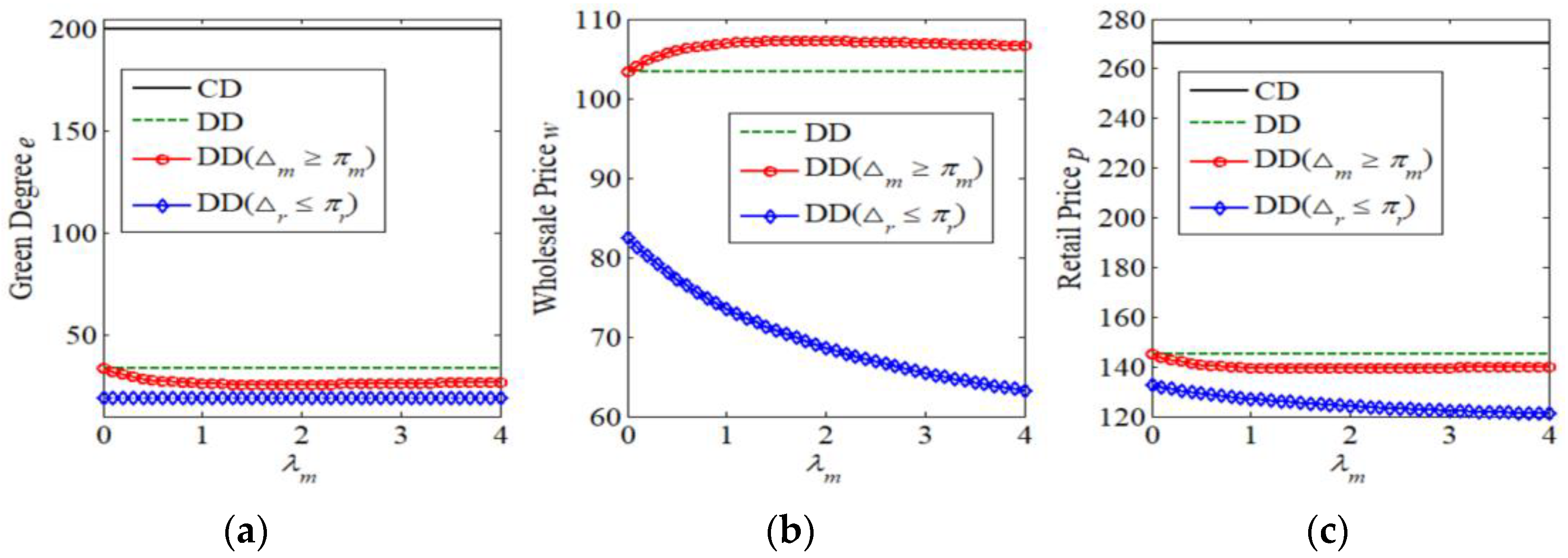
The effects of Signify’s loss aversion on green degree, wholesale price and retail price are shown in Figure 3a–c, respectively. In Figure 3a, product green degree in DD(∆mπm) is decreasing first in λm and then increasing in λm. while product green degree in DD(∆rπr) is increasing in λm. That is, in DD(∆mπm), with the increase of Signify’s levels of loss aversion, Signify first reduces product green degree and improves product green degree; while in DD(∆rπr) Signify improves gradually product green degree with the increase of Signify’s levels of loss aversion. In addition, in Figure 3a product green degree in DD(∆mπm) is higher than that in DD(∆rπr) and lower than that in CD and DD. In Figure 3b, the wholesale price in DD(∆mπm) is increasing first in λm and then decreasing in λm. while the wholesale price in DD(∆rπr) is decreasing first in λm. That is, in DD(∆mπm), with the increase of Signify’s levels of loss aversion, Signify first improves the wholesale price and decrease the wholesale price; while in DD(∆rπr) Signify reduces gradually the wholesale price with the increase of Signify’s levels of loss aversion. In addition, in Figure 3b the wholesale price in DD(∆mπm) is higher than that in DD(∆rπr). In Figure 3c, the retailer price in DD(∆mπm) is decreasing first in λm and then increasing in λm, while the retailer price in DD(∆rπr) is decreasing in λm. According to Figure 3c, the retail price is the highest in CD, the retail price in DD is the second highest, followed by in DD(∆mπm), it is the lowest in DD(∆rπr). From Figure 3a,c, it follows that the loss-averse preferences of manufacturer decrease product green degree and the retail price compared to CD and DD, and that product green degree and the retail price in the green supply chain with the retailer incurring loss is less than that in the green supply chain with the manufacturer incurring loss. In addition, according to Figure 3b, the loss-averse preference of manufacturer increases the wholesale price in the green supply chain with the manufacturer incurring loss compared to DD, while it reduces the wholesale price in the green supply chain the retailer incurring loss compared to DD.
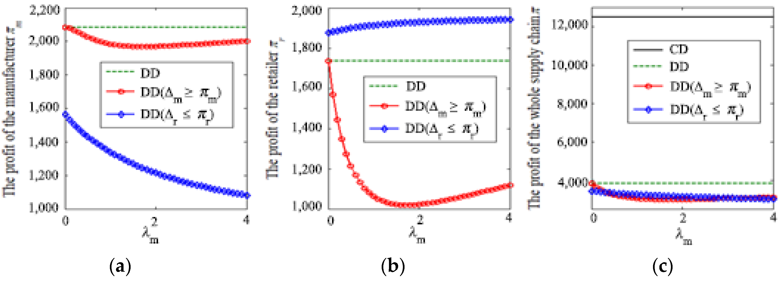
The effects of Signify’s loss aversion on the profits of Signify, retailer and the supply chain system are shown in Figure 4a–c, respectively. Figure 4a shows the changes of Signify’s profit with Signify’s levels of loss aversion. From Figure 4a, it follows that Signify’s profit in DD(∆mπm) is decreasing first in λm and then increasing in λm and Signify’s profit in DD(∆rπr) is decreasing in λm. In addition, in Figure 4a Signify’s profit in DD(∆mπm) is higher than that in DD(∆rπr), while the former is lower than Signify’s profit in DD. Figure 4b shows the changes of the retailer’s profit with Signify’s levels of loss aversion. According to Figure 4b, the retailer’s profit in DD(∆mπm) is decreasing first in λm and then increasing in λm and the retailer’s profit in DD(∆rπr) is increasing in λm. On the other hand, in Figure 4b the retailer’s profit in DD(∆rπr) is the highest, followed by that in DD, and it is the lowest in DD(∆mπm). Figure 4c shows the changes of the overall profit with Signify’s levels of loss aversion. By Figure 4c, the overall profit in DD(∆mπm) is decreasing first in λm and then increasing in λm and the overall profit in DD(∆rπr) is decreasing in λm. In Figure 4c, the overall profit in CD is the highest. After the overall profit in CD, the overall profit in DD is the second highest, followed by that in DD(∆mπm) and in DD(∆rπr) it is the lowest if Signify’s level of loss aversion is sufficiently low or high (otherwise, followed by that in DD(∆rπr) and in DD(∆mπm) it is the lowest). By Figure 4a,c), in DD(∆mπm), if Signify’s levels of loss aversion are low, Signify as well as the retailer are hurt by Signify’s levels of loss aversion; otherwise, they benefit from it. In DD(∆rπr), Signify suffers from its own level of loss aversion, while the retailer benefits from it. In addition, in Figure 4b, compared to DD, the retailer’s profit in DD(∆rπr) is higher than that in DD, while the retailer’s profit in DD(∆mπm) is lower than that in DD.
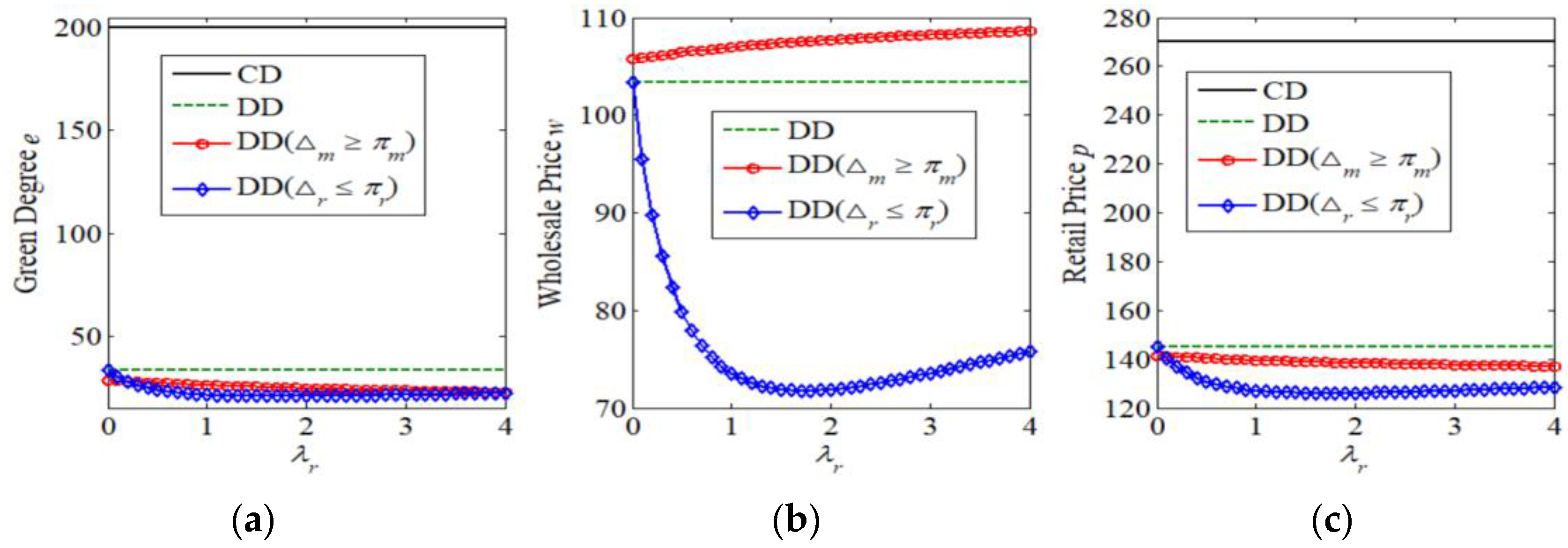
The effects of retailer’s loss aversion on green degree, wholesale price and retail price are shown in Figure 5a–c, respectively. In Figure 5a, while product green degree in DD(∆mπm) is decreasing first in λr, while product green degree in DD(∆rπr) is decreasing first in λr and then increasing in λr. That is, in DD(∆mπm), with the increase of the retailer’s levels of loss aversion, Signify will reduce product green degree; while in DD(∆rπr), Signify first reduces product green degree and improve product green degree. In Figure 5a, product green degree in CD is the highest, it in DD is the second highest after in CD, followed by product green degree in DD, and it is the lowest in DD(∆mπm) if the retailer’s levels of loss aversion are sufficiently low or high. Otherwise, it is the lowest in DD(∆rπr). In Figure 5b, the wholesale price in DD(∆mπm) is increasing first in λr, while the wholesale price in DD(∆rπr) is decreasing first in λr and then increasing in λr. That is, in DD(∆mπm), with the increase of the retailer’s levels of loss aversion, Signify will increase the wholesale price, while in DD(∆rπr) Signify first decreases the wholesale price and increases the wholesale price. In Figure 5b the wholesale price in DD(∆mπm) is higher than that in DD, while the latter is higher than that in DD(∆rπr). In Figure 5c, the retailer’s price in DD(∆mπm) is decreasing in λr, while the retailer’s price in DD(∆rπr) is decreasing first in λm and then increasing in λr. According to Figure 5c, the retail price is the highest in CD, the retail price in DD is the second highest, followed by that in DD(∆rπr), and it is the lowest in DD(∆mπm) if the retailer’s levels of loss aversion is sufficiently low. Otherwise, it is the lowest in DD(∆rπr). From Figure 5a,c, it follows that the loss-averse preferences of the retailer decrease product green degree and the retail price compared to CD and DD, and that the size of product green degrees and the retail prices in DD(∆mπm) and DD(∆rπr) depends on the retailer’s levels of loss aversion. In addition, according to Figure 5b, the loss-averse preference of the retailer increases the wholesale price in the green supply chain with the manufacturer incurring loss compared to DD, while it reduces the wholesale price in the green supply chain with the retailer incurring loss compared to DD.
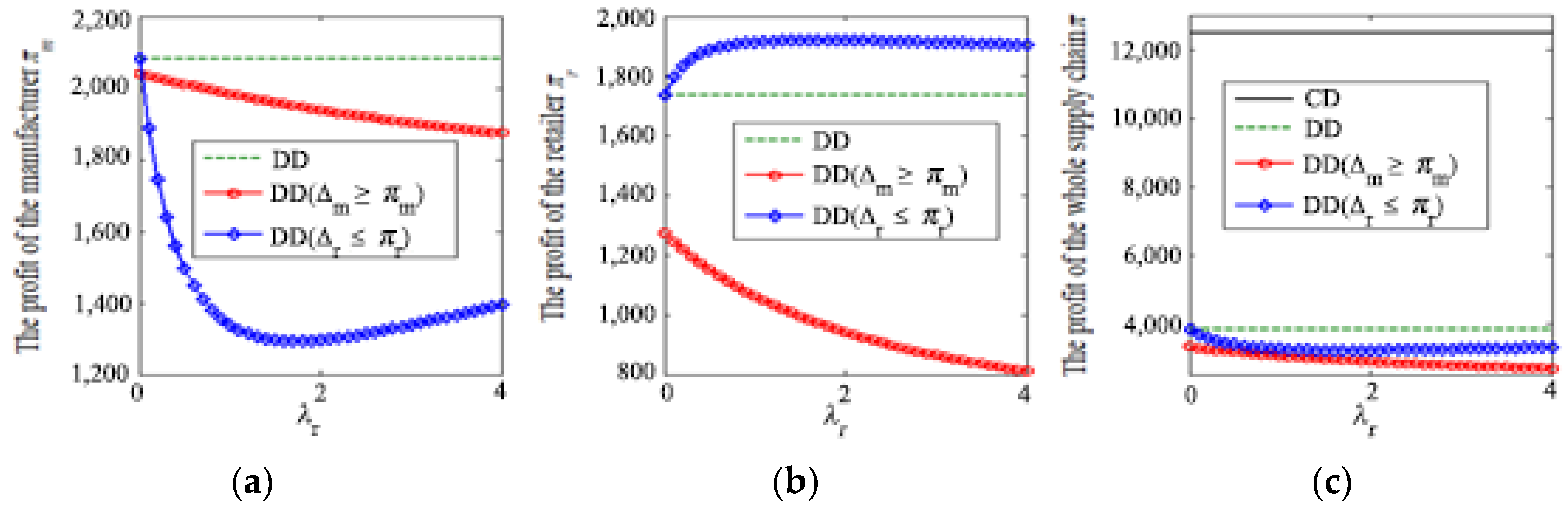
The effects of retailer’s loss aversion on the profits of Signify, retailer and the supply chain system are shown in Figure 6a–c, respectively. Figure 6a shows the changes of Signify’s profit with the retailer’s levels of loss aversion. From Figure 6a, Signify’s profit in DD(∆mπm) is decreasing in λr. and Signify’s profit in DD(∆rπr) is decreasing first in λr and then increasing in λr. In Figure 6a, Signify’s is the highest in DD. If the retailer’s levels of loss aversion are sufficiently low, the lowest profit for Signify is in DD(∆mπm); otherwise, the lowest profit for Signify is in DD(∆rπr). Figure 6b shows the changes of the retailer’s profit with its own levels of loss aversion. From Figure 6b, the retailer’s profit in DD(∆mπm) is decreasing in λr. and the retailer’s profit in DD(∆rπr) is increasing first in λr and then decreasing in λr. In Figure 6b, the retailer’s profit in DD(∆rπr) is the highest, followed by the retailer’s profit in DD, and it is lowest in DD(∆mπm). Figure 6c shows the changes of the overall profit with the retailer’s levels of loss aversion. By Figure 6c, the overall profit in DD(∆rπr) is decreasing in λr, and the overall profit in DD(∆rπr) is decreasing first in λr and then increasing in λr and In Figure 6c, the overall profit in CD is the highest. After the overall profit in CD, the overall profit in DD is the second highest, followed by that in DD(∆rπr), it in DD(∆mπm) is the lowest. By Figure 6a,c, in DD(∆mπm), Signify as well as the retailer suffer from the retailer’s levels of loss aversion. In DD(∆rπr), if the retailer’s levels of loss aversion are low, Signify is hurt by the retailer’s levels of loss aversion, while the retailer benefits from it; if the retailer’s levels of loss aversion are high, Signify benefits from the retailer’s levels of loss aversion, while the retailer is hurt by it. In addition, in Figure 6b, compared to DD, the retailer’s profit in DD(∆rπr) is higher than that in DD, while the retailer’s profit in DD(∆mπm) is lower than that in DD.

6. Managerial Insights

When the manufacturer incurs a loss, the manufacturer with low (high) loss-aversion levels will increase the wholesale price and the loss-averse retailer will increase (decrease) the retail price if GECP is sufficiently low (high). On the other hand, when the retailer incurs a loss, the manufacturer with loss aversion will decrease the wholesale price, which leads to a low retail price for the retailer. A retailer with low (high) loss-aversion levels will decrease (increase) the wholesale price, which leads to a low (high) retail price.
When the manufacturer incurs a loss, a lower (higher) loss aversion for the manufacturer will lead to a higher product green degree if the loss-aversion level of the manufacturer is low (high), while the retailer with loss aversion will lead to a lower product green degree. When the retailer incurs a loss, the manufacturer with loss aversion will lead to a lower product green degree, while a lower (higher) loss aversion for the retailer will lead to a higher product green degree if the loss-aversion level of the manufacturer is low (high).
When the members are loss averse, the manufacturer is reluctant to improve the product green degree. When the manufacturer incurs a loss, compared with pricing decision of the rational GSC members, the manufacturer will set a high (low) the wholesale price and the retailer will set a high (low) retail price if GECP is low (high). When the retailer incurs a loss, compared with pricing decision of the rational GSC members, the manufacturer and the retailer will set low wholesale and retail prices.

7. Conclusions

In this paper, we restrict ourselves to a two-echelon GSC with a single loss-averse manufacturer and a single loss-averse retailer. Shalev’s [23] model of loss aversion is adopted to formulate the loss-aversion preferences for the manufacturer and the retailer, whose loss-aversion reference dependence is formalized using Nash bargaining solution. A decision model of the two-echelon GSC with loss aversion is constructed. Then the associated equilibrium strategies are calculated. We discuss the impacts of the GSC members’ levels of loss aversion and GECP on the GSC decisions, such as retail price, wholesale price and product green degree. We also analyze the effects of the GSC members’ levels of loss aversion and GECP on profits, including the profits for the manufacturer as well as the retailer and the profit of the whole GSC. Finally, a comparative analysis of outcomes with respect to GECP and members’ levels of loss aversion are performed in four scenarios (i.e., CD, DD, DD(∆mπm) and DD(∆rπr)) by using numerical stimulation.
In DD(∆rπr) and DD (∆mπm), product green degree is lower than that in the other two scenarios. GECP has a critical impact on the retail price and the wholesale price. In DD (∆mπm), the wholesale (retail) price is higher than that in DD (and CD) if GECP is low, while it is less than that in DD (DD and CD) if GECP is high. In DD(∆rπr), the retail price is higher than that in CD and less than that in DD, if GECP is sufficiently low; otherwise, it is the lowest in three scenarios, while in DD(∆rπr) the wholesale price is less than that in DD regardless of GECP.
Furthermore, the profits of the manufacturer and the retailer in DD(∆mπm) are less than that in DD. The profit of the whole GSC in CD is higher than that in DD, while the latter is higher than that in DD(∆mπm). Maximizing the profits of the GSC members leads to the decrease of the profit of the whole GSC. Furthermore, once the manufacturer occurs loss, its loss-averse preference causes it to pay more attention to loss than gain, which further decreases the profit of the whole GSC. In DD(∆rπr), the conclusions for the manufacturer and the whole GSC are identical to those in DD(∆mπm). In DD(∆rπr), the retailer’s profit is higher (less) than that in DD if GECP is low (high).
Moreover, in DD(∆mπm), the retail price and the wholesale price increase (decrease) with the retailer’s levels of loss aversion if GECP is low (high), but the changes of the retail price and the wholesale price with the manufacturer’s levels of loss aversion depend on GECP as well as the gap between the levels of members’ loss aversion. In DD(∆rπr), the retail price and the wholesale price decrease with the manufacturer’s levels of loss aversion, while the changes of the retail price and the wholesale price with the manufacturer’s levels of loss aversion depend on the gap between the levels of members’ loss aversion. Product green degree is decreasing monotonically with the levels of loss aversion of the GSC member without loss, but the changes of product green degree with the levels of loss aversion of the GSC member with loss depend on the gap between the levels of the GSC members’ loss aversion.
Finally, in DD(∆mπm), the GSC members’ profits are decreasing monotonically with the levels of loss aversion of the retailer. In DD(∆mπm), the changes of the GSC member’s profit with the levels of loss aversion of the manufacturer depend on the gap between the levels of members’ loss aversion. In DD(∆rπr), the manufacturer’s profit is decreasing monotonically its levels of loss aversion, but the changes of manufacturer’s profit with the levels of loss aversion of the retailer depend on the gap between the levels of the GSC members’ loss aversion. In DD(∆rπr), the retailer’s profit is decreasing (increasing) monotonically the levels of loss aversion of the manufacturer if GECP is low (high), while the changes of the retailer’s profit with its levels of loss aversion depend on GECP as well as the gap between the levels of members’ loss aversion.
The present paper extends the study of the GSC to incorporate loss aversion, considering a single loss-averse manufacturer and a single loss-averse retailer. Although our study contributes to the extant literature on GSCM, the developed model does not take into account governmental interventions, since environmental issues are acquiring increasing importance from governments around the world, and a series of policies with respect to environmental protection have been promulgated. Thus, an interesting extension of our study would be to consider the governmental interventions in the future. Another interesting extension of our study would be what will happen when technology or green degree requirements change over time.

Author Contributions

Conceptualization, Z.F.; Formal analysis, W.Y. and Z.F.; Funding acquisition, Z.F., C.T. and Y.Y.; Methodology, W.Y. and Z.F.; Project administration, C.T. and Y.Y.; Supervision, C.T. and Y.Y.; Writing—original draft, Z.F.; Writing—review & editing, W.Y. All authors have read and agreed to the published version of the manuscript.

Funding

This work was partly supported by the National Natural Science Foundation of China (Nos. 71971218 and U1904210), Doctoral fund of Henan Polytechnic University (760207/025), and Special project for key R & D and promotion in Henan Province (212400410323).

Institutional Review Board Statement

Not applicable.

Informed Consent Statement

Not applicable.

Data Availability Statement

The study did not report any data.

Conflicts of Interest

The authors declare no conflict of interest.

Appendix A

Proof of Lemma 1.
By Nash’s axiomatic definition [37,38] and the definition of stable reference point in Nash bargaining with loss aversion [65], the stable reference point pairs (∆m, ∆r) is to maximize Nash product urum, i.e.,
max Δ m , Δ r [ ( 1 + λ r ) π r λ r max { π r , Δ r } ] [ ( 1 + λ m ) π m λ m max { π m , Δ m } ] s . t . Δ m + Δ r = π s c .     Δ m , Δ r ( 0 , π s c ] .
From Shalev’s [65] Theorem 3.2, it follows that there is a tangent to the linear function Δ m + Δ r = π s c through the point (∆m, ∆r) with slope Δ r ( 1 + λ r ) / Δ m ( 1 + λ m ) . Thus, we have:
Δ r ( 1 + λ r ) Δ m ( 1 + λ m ) = 1
By combining with Δ m + Δ r = π s c , we have:
Δ m = ( 1 + λ r ) π s c 2 + λ m + λ r ; Δ r = ( 1 + λ m ) π s c 2 + λ m + λ r .
Proof of Theorem 1.
By Equations (5) and (11), we have:
p D p = 2 h ( a c ) ( h τ 2 ) ( 2 h τ 2 ) ( 4 h τ 2 ) .
By Equations (11) and (23), we have:
p D , Δ m p D = 2 h λ m ( 1 + λ r ) ( a c ) ( h τ 2 ) 2 { h [ 4 ( 1 + λ m ) 2 + 4 ( 1 + λ r ) + 2 λ m ( 1 + λ r ) ] [ ( 1 + λ m ) 2 + ( 1 + λ r ) ] τ 2 } ( 4 h τ 2 )
Since 0 < τ 2 / h < 2 , we have:
{ p D , Δ m > p D > p p D , Δ m = p D = p p D , Δ m < p D < p 0 < τ 2 / h < 1 τ 2 / h = 1 1 < τ 2 / h < 2
By Equations (11) and (33), we have:
p D , Δ r p D = 3 h τ 2 λ r ( 1 + λ m ) ( a c ) { 4 h ( 1 + λ r ) ( 2 + λ m + λ r ) [ ( 1 + λ r ) 2 + ( 1 + λ m ) ] τ 2 } ( 4 h τ 2 ) < 0 .
By Equations (5) and (33), we have:
p D , Δ r p = h ( a c ) { h ( 1 + λ r ) ( 2 + λ m + λ r ) [ ( 1 + λ r ) ( 2 + λ m + λ r ) + λ r ( 1 + λ m ) ] τ 2 } { 4 h ( 1 + λ r ) ( 2 + λ m + λ r ) [ ( 1 + λ r ) 2 + ( 1 + λ m ) ] τ 2 } ( 2 h τ 2 )
For simplicity, let ψ = 1 λ r ( 1 + λ m ) ( 1 + λ r ) ( 2 + λ m + λ r ) + λ r ( 1 + λ m ) . Then we have:
{ p D > p D , Δ r > p p D > p D , Δ r = p p D > p > p D , Δ r p D = p > p D , Δ r p > p D > p D , Δ r 0 < τ 2 / h < ψ τ 2 / h = ψ ψ < τ 2 / h < 1 τ 2 / h = 1 1 < τ 2 / h < 2 .
Proof of Proposition 1.
Differentiating p D , Δ m with respect to λm and λr yields:
d p D , Δ m d λ m = 2 h ( a c ) ( 1 + λ r ) ( λ m 2 λ r 2 ) ( h τ 2 ) { h [ 4 ( 1 + λ m ) 2 + 4 ( 1 + λ r ) + 2 λ m ( 1 + λ r ) ] [ ( 1 + λ m ) 2 + ( 1 + λ r ) ] τ 2 } 2
When 0 < τ 2 / h < 1 , we have:
d p D , Δ m d λ m { > 0 λ m < λ r + 2 < 0 λ m > λ r + 2
When 1 < τ 2 / h < φ , we have:
d p D , Δ m d λ m { < 0 λ m < λ r + 2 > 0 λ m > λ r + 2
d p D , Δ m d λ r = 2 h ( a c ) λ m ( 1 + λ m ) 2 ( h τ 2 ) { h [ 4 ( 1 + λ m ) 2 + 4 ( 1 + λ r ) + 2 λ m ( 1 + λ r ) ] [ ( 1 + λ m ) 2 + ( 1 + λ r ) ] τ 2 } 2 { > 0 0 < τ 2 / h < 1 < 0 1 < τ 2 / h < φ
Differentiating p D , Δ r with respect to λm and λr yields:
d p D , Δ r d λ m = 3 h τ 2 ( a c ) λ r ( 1 + λ r ) 2 { 4 h ( 1 + λ r ) ( 2 + λ m + λ r ) [ ( 1 + λ r ) 2 + ( 1 + λ m ) ] τ 2 } 2 < 0
and
d p D , Δ r d λ r = 3 h τ 2 ( a c ) ( 1 + λ m ) ( λ r 2 λ m 2 ) { 4 h ( 1 + λ r ) ( 2 + λ m + λ r ) [ ( 1 + λ r ) 2 + ( 1 + λ m ) ] τ 2 } 2 { > 0 λ r > λ m + 2 < 0 λ r < λ m + 2
Proof of Theorem 2.
From Equations (9) and (21), it follows that:
w D , Δ m w D = λ m ( 1 + λ r ) h ( a c ) ( 2 h τ 2 ) 8 { h [ 4 ( 1 + λ m ) 2 + 4 ( 1 + λ r ) + 2 λ m ( 1 + λ r ) ] [ ( 1 + λ m ) 2 + ( 1 + λ r ) ] τ 2 } ( 4 h τ 2 )
Since 0 < τ 2 / h < 4 , then we have
w D , Δ m w D = { > 0 = 0 < 0 0 < τ 2 / h < 2 τ 2 / h = 2 2 < τ 2 / h < 4
From Equations (9) and (31), it follows that:
w D , Δ r w D = 2 λ m ( 1 + λ r ) h 2 ( a c ) { 4 h ( 1 + λ r ) ( 2 + λ m + λ r ) [ ( 1 + λ r ) 2 + ( 1 + λ m ) ] τ 2 } ( 4 h τ 2 ) < 0 .
Proof of Proposition 2.
Differentiating w D , Δ m with respect to λm and λr yields:
d w D , Δ m d λ m = 2 h ( a c ) ( 1 + λ r ) ( λ m 2 λ r 2 ) ( 2 h τ 2 ) { h [ 4 ( 1 + λ m ) 2 + 4 ( 1 + λ r ) + 2 λ m ( 1 + λ r ) ] [ ( 1 + λ m ) 2 + ( 1 + λ r ) ] τ 2 } 2
When 0 < τ 2 / h < 2 , we have:
d w D , Δ m d λ m { > 0 λ m < λ r + 2 < 0 λ m > λ r + 2
When 2 < τ 2 / h < φ , we have:
d w D , Δ m d λ m { < 0 λ m < λ r + 2 > 0 λ m > λ r + 2
d w D , Δ m d λ r = 2 h ( a c ) λ m ( 1 + λ m ) 2 ( 2 h τ 2 ) { h [ 4 ( 1 + λ m ) 2 + 4 ( 1 + λ r ) + 2 λ m ( 1 + λ r ) ] [ ( 1 + λ m ) 2 + ( 1 + λ r ) ] τ 2 } 2 { > 0 0 < τ 2 / h < 2 < 0 2 < τ 2 / h < φ
Differentiating w D , Δ r with respect to λm and λr yields:
d w D , Δ r d λ m = 8 h 2 ( a c ) λ r ( 1 + λ r ) { 4 h ( 1 + λ r ) ( 2 + λ m + λ r ) [ ( 1 + λ r ) 2 + ( 1 + λ m ) ] τ 2 } 2 < 0
and
d w D , Δ r d λ r = 8 h 2 ( a c ) ( 1 + λ m ) ( λ r 2 λ m 2 ) { 4 h ( 1 + λ r ) ( 2 + λ m + λ r ) [ ( 1 + λ r ) 2 + ( 1 + λ m ) ] τ 2 } 2 { > 0 λ r > λ m + 2 < 0 λ r < λ m + 2 .
Proof of Theorem 3.
By Equations (4) and (10), and combining with 0 < τ 2 / h < 2 yields:
e D e = 2 τ h ( a c ) τ ( 4 h τ 2 ) ( 2 h τ 2 ) < 0 .
By Equations (10) and (22), and combining with 0 < τ 2 / h < 2 yields:
e D , Δ m e D = λ m ( 1 + λ r ) τ h ( a c ) 2 { h [ 4 ( 1 + λ m ) 2 + 4 ( 1 + λ r ) + 2 λ m ( 1 + λ r ) ] [ ( 1 + λ m ) 2 + ( 1 + λ r ) ] τ 2 } ( 4 h τ 2 ) < 0
By Equations (10) and (32), and combining with 0 < τ 2 / h < 2 yields:
e D , Δ r e D = 4 τ h λ r ( 1 + λ m ) ( a c ) { 4 h ( 1 + λ r ) ( 2 + λ m + λ r ) [ ( 1 + λ r ) 2 + ( 1 + λ m ) ] τ 2 } ( 4 h τ 2 ) < 0 .
Proof of Proposition 3.
Differentiating e D , Δ m with respect to λm and λr yields:
d e D , Δ m d λ m = 2 h τ ( a c ) ( 1 + λ r ) ( λ m 2 λ r 2 ) { h [ 4 ( 1 + λ m ) 2 + 4 ( 1 + λ r ) + 2 λ m ( 1 + λ r ) ] [ ( 1 + λ m ) 2 + ( 1 + λ r ) ] τ 2 } 2 { < 0 λ m < λ r + 2 > 0 λ m > λ r + 2
and
d e D , Δ m d λ r = 2 h τ ( a c ) λ m ( 1 + λ m ) 2 { h [ 4 ( 1 + λ m ) 2 + 4 ( 1 + λ r ) + 2 λ m ( 1 + λ r ) ] [ ( 1 + λ m ) 2 + ( 1 + λ r ) ] τ 2 } 2 < 0
Differentiating e D , Δ r with respect to λm and λr yields:
d e D , Δ r d λ m = 4 h τ ( a c ) λ r ( 1 + λ r ) 2 { 4 h ( 1 + λ r ) ( 2 + λ m + λ r ) [ ( 1 + λ r ) 2 + ( 1 + λ m ) ] τ 2 } 2 < 0
and
d e D , Δ r d λ r = 4 h τ ( a c ) ( 1 + λ m ) ( λ r 2 λ m 2 ) { 4 h ( 1 + λ r ) ( 2 + λ m + λ r ) [ ( 1 + λ r ) 2 + ( 1 + λ m ) ] τ 2 } 2 { > 0 λ r > λ m + 2 < 0 λ r < λ m + 2
Proof of Theorem 4.
By Equations (12) and (24), we have:
π m , D , Δ m π m D = h 3 λ m 2 ( 1 + λ r ) 2 ( a c ) 2 { h [ 4 ( 1 + λ m ) 2 + 4 ( 1 + λ r ) + 2 λ m ( 1 + λ r ) ] [ ( 1 + λ m ) 2 + ( 1 + λ r ) ] τ 2 } 2 ( 4 h τ 2 ) < 0 .
By Equations (13) and (25), we have:
π r , D , Δ m π r D = 4 h 3 λ m ( 1 + λ r ) { [ 4 ( λ m 2 + 2 λ m + λ r + 2 ) + λ m ( 1 + λ r ) ] h ( λ m 2 + 2 λ m + λ r + 2 ) τ 2 } ( a c ) 2 { h [ 4 ( 1 + λ m ) 2 + 4 ( 1 + λ r ) + 2 λ m ( 1 + λ r ) ] [ ( 1 + λ m ) 2 + ( 1 + λ r ) ] τ 2 } 2 ( 4 h τ 2 ) 2 < 0 .
By Equations (6) and (14), we have:
π s c D π s c ( p , e ) = 2 h 3 ( a c ) 2 ( 4 h τ 2 ) 2 ( 2 h τ 2 ) < 0 .
By Equations (14) and (26), we have:
π s c , D , Δ m π s c D = 4 h 3 λ m ( 1 + λ r ) { 2 [ 2 ( λ m 2 + λ m λ r + 5 λ m + 2 λ r + 4 ) + λ m ( 1 + λ r ) ] h ( λ m 2 + λ m λ r + 5 λ m + 2 λ r + 4 ) τ 2 } ( a c ) 2 { h [ 4 ( 1 + λ m ) 2 + 4 ( 1 + λ r ) + 2 λ m ( 1 + λ r ) ] [ ( 1 + λ m ) 2 + ( 1 + λ r ) ] τ 2 } 2 ( 4 h τ 2 ) 2 < 0 .
By Equations (12) and (34), we have:
π m , D , Δ r π m D = 2 h 2 λ r ( 1 + λ m ) ( a c ) 2 { 4 h ( 1 + λ r ) ( 2 + λ m + λ r ) [ ( 1 + λ r ) 2 + ( 1 + λ m ) ] τ 2 } ( 4 h τ 2 ) < 0 .
By Equations (13) and (35), we have:
π r , D , Δ r π r D = h 2 λ r ( 1 + λ m ) { [ 4 ( 1 + λ r ) ( λ m + λ r + 2 ) ( 2 h τ 2 ) ( 4 h τ 2 ) λ r ( 1 + λ m ) ] τ 4 } ( a c ) 2 { 4 h ( 1 + λ r ) ( 2 + λ m + λ r ) [ ( 1 + λ r ) 2 + ( 1 + λ m ) ] τ 2 } 2 ( 4 h τ 2 ) 2 .
There exists a threshold t for τ 2 / h depending on λm and λr such that:
π r , D , Δ r π r D { > 0 = 0 < 0 0 τ 2 / h < t τ 2 / h = t t τ 2 / h < 4
By Equations (14) and (36), we have:
π s c , D , Δ r π s c D = h 2 τ 2 λ r ( 1 + λ m ) { 8 ( 2 λ m λ r + λ r 2 + λ m + 4 λ r + 2 ) h ( 3 λ m λ r + 2 λ r 2 + 2 λ m + 7 λ r + 4 ) τ 2 } ( a c ) 2 { 4 h ( 1 + λ r ) ( 2 + λ m + λ r ) [ ( 1 + λ r ) 2 + ( 1 + λ m ) ] τ 2 } 2 ( 4 h τ 2 ) 2 < h 2 τ 2 λ r ( 1 + λ m ) { 8 h 2 τ 2 } ( a c ) 2 { 4 h ( 1 + λ r ) ( 2 + λ m + λ r ) [ ( 1 + λ r ) 2 + ( 1 + λ m ) ] τ 2 } 2 ( 4 h τ 2 ) 2 < 0 .
Proof of Proposition 4.
Differentiating π m , D , Δ m with respect to λm and λr yields:
d π m , D , Δ m d λ m = 2 h 3 ( a c ) 2 λ m ( 1 + λ r ) 2 ( λ m 2 λ r 2 ) { h [ 4 ( 1 + λ m ) 2 + 4 ( 1 + λ r ) + 2 λ m ( 1 + λ r ) ] [ ( 1 + λ m ) 2 + ( 1 + λ r ) ] τ 2 } 3 { > 0 λ m > λ r + 2 < 0 λ m < λ r + 2
d π m , D , Δ m d λ r = 4 h 3 ( a c ) 2 λ m 2 ( 1 + λ m ) 2 ( 1 + λ r ) { h [ 4 ( 1 + λ m ) 2 + 4 ( 1 + λ r ) + 2 λ m ( 1 + λ r ) ] [ ( 1 + λ m ) 2 + ( 1 + λ r ) ] τ 2 } 3 < 0
Differentiating π r , D , Δ m with respect to λm and λr yields:
d π r , D , Δ m d λ m = 4 h 3 ( a c ) 2 ( 1 + λ r ) ( λ m 2 + 2 λ m + λ r + 2 ) ( λ m 2 λ r 2 ) { h [ 4 ( 1 + λ m ) 2 + 4 ( 1 + λ r ) + 2 λ m ( 1 + λ r ) ] [ ( 1 + λ m ) 2 + ( 1 + λ r ) ] τ 2 } 3 { > 0 λ m > λ r + 2 < 0 λ m < λ r + 2
d π r , D , Δ m d λ r = 4 h 3 ( a c ) 2 λ m ( 1 + λ m ) 2 ( λ m 2 + 2 λ m + λ r + 2 ) { h [ 4 ( 1 + λ m ) 2 + 4 ( 1 + λ r ) + 2 λ m ( 1 + λ r ) ] [ ( 1 + λ m ) 2 + ( 1 + λ r ) ] τ 2 } 3 < 0
Differentiating π m , D , Δ r with respect to λm and λr yields:
d π m , D , Δ r d λ m = 2 h 2 ( a c ) 2 λ r ( 1 + λ r ) 2 { 4 h ( 1 + λ r ) ( 2 + λ m + λ r ) [ ( 1 + λ r ) 2 + ( 1 + λ m ) ] τ 2 } 3 < 0
d π m , D , Δ r d λ r = 2 h 2 ( a c ) 2 ( 1 + λ m ) ( λ r 2 λ m 2 ) { 4 h ( 1 + λ r ) ( 2 + λ m + λ r ) [ ( 1 + λ r ) 2 + ( 1 + λ m ) ] τ 2 } 3 { > 0 λ r > λ m + 2 < 0 λ r < λ m + 2
Differentiating π r , D , Δ m with respect to λm and λr,
d π r , D , Δ r * d λ m = 2 h 2 ( a c ) 2 λ r ( 1 + λ r ) 2 [ 4 ( 1 + λ r ) ( 2 + λ m + λ r ) h ( 3 λ m λ r + 2 λ r 2 + 2 λ m + 7 λ r + 4 ) τ 2 ] { 4 h ( 1 + λ r ) ( 2 + λ m + λ r ) [ ( 1 + λ r ) 2 + ( 1 + λ m ) ] τ 2 } 3 = { < 0 0 < τ 2 / h < θ > 0 θ < τ 2 / h < ϑ
where θ = 4 ( 1 + λ r ) ( 2 + λ m + λ r ) 3 λ m λ r + 2 λ r 2 + 2 λ m + 7 λ r + 4 . and
d π r , D , Δ r * d λ r = 2 h 2 ( a c ) 2 ( 1 + λ r ) ( λ r 2 λ m 2 ) [ 4 ( 1 + λ r ) ( 2 + λ m + λ r ) h ( 3 λ m λ r + 2 λ r 2 + 2 λ m + 7 λ r + 4 ) τ 2 ] { 4 h ( 1 + λ r ) ( 2 + λ m + λ r ) [ ( 1 + λ r ) 2 + ( 1 + λ m ) ] τ 2 } 3
For 0 < τ 2 / h < θ , we have:
d π r , D , Δ r d λ r { < 0 λ r > λ m + 2 > 0 λ r < λ m + 2
For θ < τ 2 / h < ϑ , we have:
d π r , D , Δ r d λ r { > 0 λ r > λ m + 2 < 0 λ r < λ m + 2

References

  1. Gleick, P.H.; Adams, R.M.; Amasino, R.M.; Anders, E.; Anderson, D.J.; Anderson, W.W.; Anselin, L.E.; Arroyo, M.K.; Asfaw, B.; Ayala, F.J.; et al. Climate Change and the Integrity of Science. Science 2010, 328, 689–690. [Google Scholar] [CrossRef] [Green Version]
  2. Wu, D.D.; Yang, L.; Olson, D.L. Green supply chain management under capital constraint. Int. J. Prod. Econ. 2019, 215, 3–10. [Google Scholar] [CrossRef]
  3. Pourjavad, E.; Shahin, A. A hybrid model for analyzing the risks of green supply chain in a fuzzy environment. J. Ind. Prod. Eng. 2020, 37, 422–433. [Google Scholar] [CrossRef]
  4. Sheu, J.-B.; Chou, Y.-H.; Hu, C.-C. An integrated logistics operational model for green-supply chain management. Transp. Res. Part E Logist. Transp. Rev. 2005, 41, 287–313. [Google Scholar] [CrossRef]
  5. Heydari, J.; Govindan, K.; Basiri, Z. Balancing price and green quality in presence of consumer environmental awareness: A green supply chain coordination approach. Int. J. Prod. Res. 2021, 59, 1957–1975. [Google Scholar] [CrossRef]
  6. Kim, S.; Foerstl, K.; Schmidt, C.G.; Wagner, S.M. Adoption of green supply chain management practices in multi-tier supply chains: Examining the differences between higher and lower tier firms. Int. J. Prod. Res. 2021, 1–18. [Google Scholar] [CrossRef]
  7. Zhao, R.; Neighbour, G.; Han, J.; McGuire, M.; Deutz, P. Using game theory to describe strategy selection for environmental risk and carbon emissions reduction in the green supply chain. J. Loss Prev. Process. Ind. 2012, 25, 927–936. [Google Scholar] [CrossRef]
  8. Li, Y.; Xie, X.; Liu, Q. Study on longitudinal emission reduction investment of supply chain and government’s subsidy policy. J. Intell. Fuzzy Syst. 2018, 34, 1177–1186. [Google Scholar] [CrossRef]
  9. Luo, J.; Chong, A.Y.-L.; Ngai, W.E.; Liu, M.J. Reprint of “Green Supply Chain Collaboration implementation in China: The mediating role of guanxi”. Transp. Res. Part E Logist. Transp. Rev. 2015, 74, 37–49. [Google Scholar] [CrossRef]
  10. Mondal, C.; Giri, B.C. Investigating strategies of a green closed-loop supply chain for substitutable products under government subsidy. J. Ind. Prod. Eng. 2021, 2021, 1–24. [Google Scholar] [CrossRef]
  11. Su, C.; Liu, X.; Du, W. Green Supply Chain Decisions Considering Consumers’ Low-Carbon Awareness under Different Government Subsidies. Sustainability 2020, 12, 2281. [Google Scholar] [CrossRef] [Green Version]
  12. Yuan, X.; Zhang, X.; Zhang, D. Research on the Dynamics Game Model in a Green Supply Chain: Government Subsidy Strategies under the Retailer’s Selling Effort Level. Complexity 2020, 2020, 3083761. [Google Scholar] [CrossRef]
  13. Govindan, K.; Kaliyan, K.M.; Kannan, D.; Haq, A. Barriers analysis for green supply chain management implementation in Indian industries using analytic hierarchy process. Int. J. Prod. Econ. 2014, 147, 555–568. [Google Scholar] [CrossRef]
  14. Mathiyazhagan, K.; Govindan, K.; NoorulHaq, A.; Geng, Y. An ISM approach for the barrier analysis in implementing green supply chain management. J. Clean. Prod. 2013, 47, 283–297. [Google Scholar] [CrossRef]
  15. Zhu, Q.; Sarkis, J.; Geng, Y. Green supply chain management in China: Pressures, practices and performance. Int. J. Oper. Prod. Manag. 2005, 25, 449–468. [Google Scholar] [CrossRef]
  16. Giri, B.C.; Mondal, C.; Maiti, T. Analysing a closed-loop supply chain with selling price, warranty period and green sensitive consumer demand under revenue sharing contract. J. Clean. Prod. 2018, 190, 822–837. [Google Scholar] [CrossRef]
  17. Nielsen, I.E.; Majumder, S.; Saha, S. Exploring the intervention of intermediary in a green supply chain. J. Clean. Prod. 2019, 233, 1525–1544. [Google Scholar] [CrossRef]
  18. Panja, S.; Mondal, S.K. Exploring a two-layer green supply chain game theoretic model with credit linked demand and mark-up under revenue sharing contract. J. Clean. Prod. 2020, 250, 119491. [Google Scholar] [CrossRef]
  19. Song, H.; Gao, X. Green supply chain game model and analysis under revenue-sharing contract. J. Clean. Prod. 2018, 170, 183–192. [Google Scholar] [CrossRef]
  20. Sun, H.; Wan, Y.; Zhang, L.; Zhou, Z. Evolutionary game of the green investment in a two-echelon supply chain under a government subsidy mechanism. J. Clean. Prod. 2019, 235, 1315–1326. [Google Scholar] [CrossRef]
  21. Kahneman, D.; Tversky, A. Prospect Theory: An analysis of decision under risk. Econometrica 1979, 47, 263–291. [Google Scholar] [CrossRef] [Green Version]
  22. Tversky, A.; Kahneman, D. Advances in prospect theory: Cumulative representation of uncertainty. J. Risk Uncertain. 1992, 5, 297–323. [Google Scholar] [CrossRef]
  23. Shalev, J. Loss aversion equilibrium. Int. J. Game Theory 2000, 29, 269–287. [Google Scholar] [CrossRef]
  24. Cui, C.; Feng, Z.; Tan, C.; Borkotokey, S. Loss Aversion Equilibrium of Bimatrix Games with Symmetric Triangular Fuzzy Payoffs. Int. J. Fuzzy Syst. 2019, 21, 892–907. [Google Scholar] [CrossRef]
  25. Driesen, B.; Perea, A.; Peters, H. On Loss Aversion in Bimatrix Games. Theory Decis. 2008, 68, 367–391. [Google Scholar] [CrossRef] [Green Version]
  26. Driesen, B.; Perea, A.; Peters, H. The Kalai–Smorodinsky bargaining solution with loss aversion. Math. Soc. Sci. 2011, 61, 58–64. [Google Scholar] [CrossRef]
  27. Driesen, B.; Perea, A.; Peters, H. Alternating offers bargaining with loss aversion. Math. Soc. Sci. 2012, 64, 103–118. [Google Scholar] [CrossRef] [Green Version]
  28. Chen, X.; Hao, G.; Li, L. Channel coordination with a loss-averse retailer and option contracts. Int. J. Prod. Econ. 2014, 150, 52–57. [Google Scholar] [CrossRef]
  29. Deng, X.; Xie, J.; Xiong, H. Manufacturer–retailer contracting with asymmetric information on retailer’s degree of loss aversion. Int. J. Prod. Econ. 2013, 142, 372–380. [Google Scholar] [CrossRef]
  30. Wang, C.X. The loss-averse newsvendor game. Int. J. Prod. Econ. 2010, 124, 448–452. [Google Scholar] [CrossRef]
  31. Wang, C.X.; Webster, S. Channel Coordination for a Supply Chain with a Risk-Neutral Manufacturer and a Loss-Averse Retailer. Decis. Sci. 2007, 38, 361–389. [Google Scholar] [CrossRef]
  32. Wu, C.; Liu, X.; Li, A. A loss-averse retailer–supplier supply chain model under trade credit in a supplier-Stackelberg game. Math. Comput. Simul. 2021, 182, 353–365. [Google Scholar] [CrossRef]
  33. Ma, L.; Xue, W.; Zhao, Y.; Zeng, Q. Loss-averse newsvendor problem with supply risk. J. Oper. Res. Soc. 2016, 67, 214–228. [Google Scholar] [CrossRef]
  34. Vipin, B.; Amit, R.K. Loss aversion and rationality in the newsvendor problem under recourse option. Eur. J. Oper. Res. 2017, 261, 563–571. [Google Scholar] [CrossRef]
  35. Wu, M.; Bai, T.; Zhu, S.X. A loss averse competitive newsvendor problem with anchoring. Omega 2018, 81, 99–111. [Google Scholar] [CrossRef]
  36. Yan, N.; He, X.; Liu, Y. Financing the capital-constrained supply chain with loss aversion: Supplier finance vs. supplier investment. Omega 2019, 88, 162–178. [Google Scholar] [CrossRef]
  37. Nash, J. The bargaining problem. Econom. J. Econom. Soc. 1950, 18, 155–162. [Google Scholar] [CrossRef]
  38. Nash, J. Two-Person Cooperative Games. Econom. J. Econom. Soc. 1953, 21, 128–140. [Google Scholar] [CrossRef]
  39. Osborne, M.J.; Rubinstein, A. A Course in Game Theory; MIT Press: Cambridge, MA, USA, 1994. [Google Scholar]
  40. Rachmilevitch, S. Fairness, Efficiency, and the Nash Bargaining Solution; Working Papers; Department of Economics, University of Haifa: Haifa, Israel, 2011. [Google Scholar]
  41. Touati, C.; Altman, E.; Galtier, J. Generalized Nash Bargaining Solution for bandwidth allocation. Comput. Netw. 2006, 50, 3242–3263. [Google Scholar] [CrossRef] [Green Version]
  42. Ghosh, D.; Shah, J. A comparative analysis of greening policies across supply chain structures. Int. J. Prod. Econ. 2012, 135, 568–583. [Google Scholar] [CrossRef]
  43. Swami, S.; Shah, J. Channel coordination in green supply chain management. J. Oper. Res. Soc. 2013, 64, 336–351. [Google Scholar] [CrossRef]
  44. Ghosh, D.; Shah, J. Supply chain analysis under green sensitive consumer demand and cost sharing contract. Int. J. Prod. Econ. 2015, 164, 319–329. [Google Scholar] [CrossRef]
  45. Zhu, W.; He, Y. Green product design in supply chains under competition. Eur. J. Oper. Res. 2017, 258, 165–180. [Google Scholar] [CrossRef]
  46. Yenipazarli, A. To collaborate or not to collaborate: Prompting upstream eco-efficient innovation in a supply chain. Eur. J. Oper. Res. 2017, 260, 571–587. [Google Scholar] [CrossRef]
  47. Bai, T.; Wu, M.; Zhu, S.X. Pricing and ordering by a loss averse newsvendor with reference dependence. Transp. Res. Part E Logist. Transp. Rev. 2019, 131, 343–365. [Google Scholar] [CrossRef]
  48. Ghosh, D.; Shah, J.; Swami, S. Product greening and pricing strategies of firms under green sensitive consumer demand and environmental regulations. Ann. Oper. Res. 2020, 290, 491–520. [Google Scholar] [CrossRef]
  49. Patra, P. Distribution of profit in a smart phone supply chain under Green sensitive consumer demand. J. Clean. Prod. 2018, 192, 608–620. [Google Scholar] [CrossRef]
  50. Gao, R.; Zhang, Z. Analysis of green supply chain considering green degree and sales effort with uncertain demand. J. Intell. Fuzzy Syst. 2020, 38, 4247–4264. [Google Scholar] [CrossRef]
  51. Liu, W.; Song, S.; Wu, C. Impact of loss aversion on the newsvendor game with product substitution. Int. J. Prod. Econ. 2013, 141, 352–359. [Google Scholar] [CrossRef]
  52. Lee, C.-Y.; Li, X.; Yu, M. The loss-averse newsvendor problem with supply options. Nav. Res. Logist. 2015, 62, 46–59. [Google Scholar] [CrossRef]
  53. Hu, B.; Meng, C.; Xu, D.; Son, Y.-J. Three-echelon supply chain coordination with a loss-averse retailer and revenue sharing contracts. Int. J. Prod. Econ. 2016, 179, 192–202. [Google Scholar] [CrossRef]
  54. Zhang, B.; Wu, D.; Liang, L.; Olson, D.L. Supply Chain Loss Averse Newsboy Model with Capital Constraint. IEEE Trans. Syst. Man, Cybern. Syst. 2016, 46, 646–658. [Google Scholar] [CrossRef]
  55. Xu, X.; Chan, C.K.; Langevin, A. Coping with risk management and fill rate in the loss-averse newsvendor model. Int. J. Prod. Econ. 2018, 195, 296–310. [Google Scholar] [CrossRef]
  56. Huang, F.; He, J.; Wang, J. Coordination of VMI supply chain with a loss-averse manufacturer under quality-dependency and marketing-dependency. J. Ind. Manag. Optim. 2019, 15, 1753–1772. [Google Scholar] [CrossRef] [Green Version]
  57. Feng, Z.; Tan, C. Pricing, Green Degree and Coordination Decisions in a Green Supply Chain with Loss Aversion. Mathematics 2019, 7, 239. [Google Scholar] [CrossRef] [Green Version]
  58. Yang, D.; Xiao, T. Coordination of a supply chain with loss-averse consumers in service quality. Int. J. Prod. Res. 2017, 55, 3411–3430. [Google Scholar] [CrossRef]
  59. Liu, C.; Lee, C.; Leung, K.H. Pricing Strategy in Dual-Channel Supply Chains with Loss-Averse Consumers. Asia-Pac. J. Oper. Res. 2019, 36, 1–22. [Google Scholar] [CrossRef]
  60. Du, S.; Zhu, Y.; Nie, T.; Yu, H. Loss-averse preferences in a two-echelon supply chain with yield risk and demand uncertainty. Oper. Res. 2018, 18, 361–388. [Google Scholar] [CrossRef]
  61. Xu, X.; Chan, F.T.; Chan, C.K. Optimal option purchase decision of a loss-averse retailer under emergent replenishment. Int. J. Prod. Res. 2018, 57, 4594–4620. [Google Scholar] [CrossRef]
  62. Liu, Z.; Anderson, T.D.; Cruz, J.M. Consumer environmental awareness and competition in two-stage supply chains. Eur. J. Oper. Res. 2012, 218, 602–613. [Google Scholar] [CrossRef]
  63. Dey, K.; Saha, S. Influence of procurement decisions in two-period green supply chain. J. Clean. Prod. 2018, 190, 388–402. [Google Scholar] [CrossRef]
  64. Wang, F.S. Research on Green Strategy of S Company’s LED Light Closed-Loop Supply Chain. Master’s Thesis, Donghua University, Shanghai, China, 2021; pp. 1–58. [Google Scholar]
  65. Shalev, J. Loss Aversion and Bargaining. Theory Decis. 2002, 52, 201–232. [Google Scholar] [CrossRef]
Figure 1. The effects of green efficiency coefficient of products (GECP) on decision variables.
Mathematics 09 03154 g001
Figure 2. The effects of GECP on profits.
Mathematics 09 03154 g002
Figure 3. The effects of Signify’s levels of loss aversion on decision variables.
Mathematics 09 03154 g003
Figure 4. The effects of Signify’s levels of loss aversion on profits.
Mathematics 09 03154 g004
Figure 5. The effects of the retailer’s levels of loss aversion on decision variables.
Mathematics 09 03154 g005
Figure 6. The effects of the retailer’s levels of loss aversion on profits.
Mathematics 09 03154 g006
Publisher’s Note: MDPI stays neutral with regard to jurisdictional claims in published maps and institutional affiliations.

