Control Method for Flexible Joints in Manipulator Based on BP Neural Network Tuning PI Controller

Abstract

With the development of robot technology, integrated joints with small volume and convenient installation have been widely used. Based on the double inertia system, an integrated joint motor servo system model considering gear angle error and friction interference is established, and a joint control strategy based on BP neural network and pole assignment method is designed to suppress the vibration of the system. Firstly, the dynamic equation of a planetary gear system is derived based on the Lagrange method, and the gear vibration of angular displacement is calculated. Secondly, the vibration displacement of the sun gear is introduced into the motor servo system in the form of the gear angle error, and the double inertia system model including angle error and friction torque is established. Then, the PI controller parameters are determined by pole assignment method, and the PI parameters are adjusted in real time based on the BP neural network, which effectively suppresses the vibration of the system. Finally, the effects of friction torque, pole damping coefficient and control strategy on the system response and the effectiveness of vibration suppression are analyzed.

1. Introduction

With the development of robot technology, the integrated joint has been widely used in robots. Compared with the traditional robot joint transmission system, the integrated joint is smaller in structure and lighter in mass. Harmonic gear is often used as a reducer in the integrated joint, and the flexible element and transmission shaft system in the harmonic reducer have torsional stiffness. The servo system with the integrated joint has certain torsional stiffness [1]. In reference [2], the joint considering torsional stiffness is called the flexible joint. The existence of joint flexibility will cause the fluctuation of output speed of the servo system. Suppress the fluctuation of output speed and improve the control accuracy of the flexible joint has become a hot issue [3,4].

To achieve accurate control of the servo system, it is necessary to establish an accurate dynamic model. A large number of scholars have discussed the dynamic modeling of flexible joint. References [5,6] believe that the flexible joint model can be equivalent to a double inertia system, and the double inertia system relies on the motor to drive the load to rotate. During load operation, the system is affected by friction torque. References [7,8] consider the influence of friction factors on the basis of the double inertia system. In addition, gears are often used in the transmission of the double inertia system. Reference [9] considers the gear reduction ratio based on the double inertia model but does not consider the dynamic performance of the gear system. Li et al. [10] established a planetary gear torsional dynamics model considering time-varying stiffness, backlash and transmission error. Li et al. [11,12] established the planetary gear system and the gear-bearing system model, respectively, and studied the influence of load and wear on the response of the system. In order to construct a more accurate dynamic model, reference [13] considers the flexibility of the load. With the deepening of the research on flexible joint modeling, nonlinear factors such as gear transmission error and friction are gradually introduced into the dynamic modeling process.

In terms of output speed fluctuation of the servo system caused by joint flexibility, the intelligent control strategy suppresses the fluctuation of speed by adjusting the input torque in real time. Typical control strategies for robot servo systems include PID control strategy, sliding mode control strategy, robust control strategy, fuzzy control strategy, neural network control strategy and so on. References [14,15] select PI method to control its parameters through a pole assignment strategy. Reference [16] designs the adaptive law of the flexible joint servo system according to the sliding mode control strategy. References [17,18] adopt robust control strategies to reduce the influence of time-varying parameters of the flexible joint. References [19,20] use fuzzy adaptive PID controller to control the flexible joint. Reference [21] uses RBF neural network to compensate the uncertain part of the servo system, thereby suppressing the fluctuation of the output speed. Regarding the control strategy of the robot servo system, the PI control strategy is still most widely used. There are many methods for parameter tuning of PI/PID controller, including the Zielger–Nicholos method, the pole tuning method, the fuzzy adaptive tuning method, the BP neural network tuning method and so on. Among them, the Z–N method and the pole tuning method can only preliminarily determine the approximate range of control parameters.

With the development of intelligent control technology, the PI control strategy with fixed parameters is gradually replaced by the PI control with variable parameters. The BP neural network and the fuzzy adaptive tuning method are suitable for accurate determination of controller parameters. However, these two control strategies need a large amount of calculation. The parameter tuning method of PI controller based on the combination of pole assignment strategy and BP neural network control strategy is to determine the range of optimal controller parameters through pole assignment strategy, and then the neural network is used to determine the optimal controller parameters. Compared with using the BP neural network alone, it can effectively reduce the amount of calculation.

A dynamic model of the flexible joint, which considers two nonlinear factors: gear transmission error and friction, is established at the beginning of the paper. Then BP neural network is utilized to tune the PI controller parameters to suppress the fluctuation of the output speed. Finally, the effectiveness of the proposed control strategy is proved by numerical simulation. The main contributions of this paper can be summarized as follows: (1) The factors of gear transmission error and friction are considered in the dynamic modeling of the flexible joint; (2) The control strategy combining the pole assignment and BP neural network is used to suppress the fluctuation of the output speed of the servo system; (3) Compared with the reference [22], the gear transmission error and friction factors are considered in the dynamic modeling process to establish a more accurate dynamic model; (4) Compared with the reference [23], the BP neural network is used to adjust the controller parameters online in real time to further reduce the error of the output speed.

The rest of this paper is organized as follows. A flexible joint dynamic model considering gear angle error and friction torque is established in the second part. In the third part, the control strategy combining the pole assignment and the BP neural network is used to control the speed of the servo system. In the fourth part, numerical simulations are carried out to verify the effectiveness of the control strategy proposed in this paper. The fifth part is the conclusion.

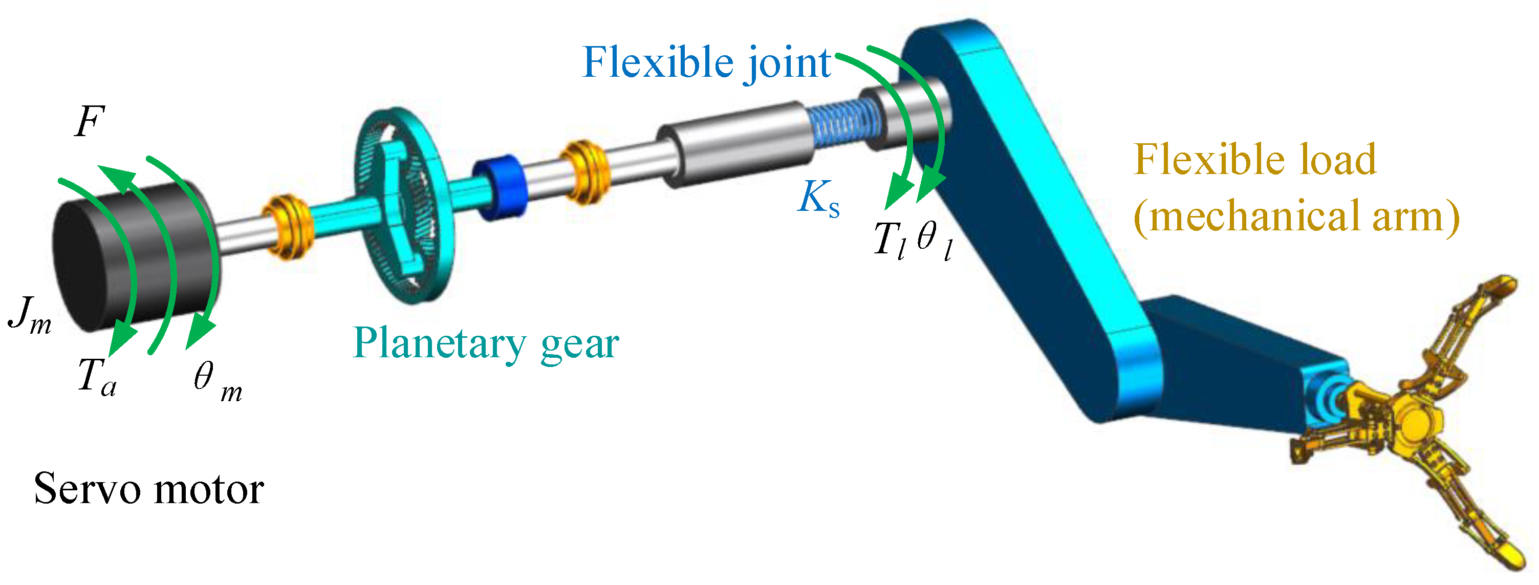
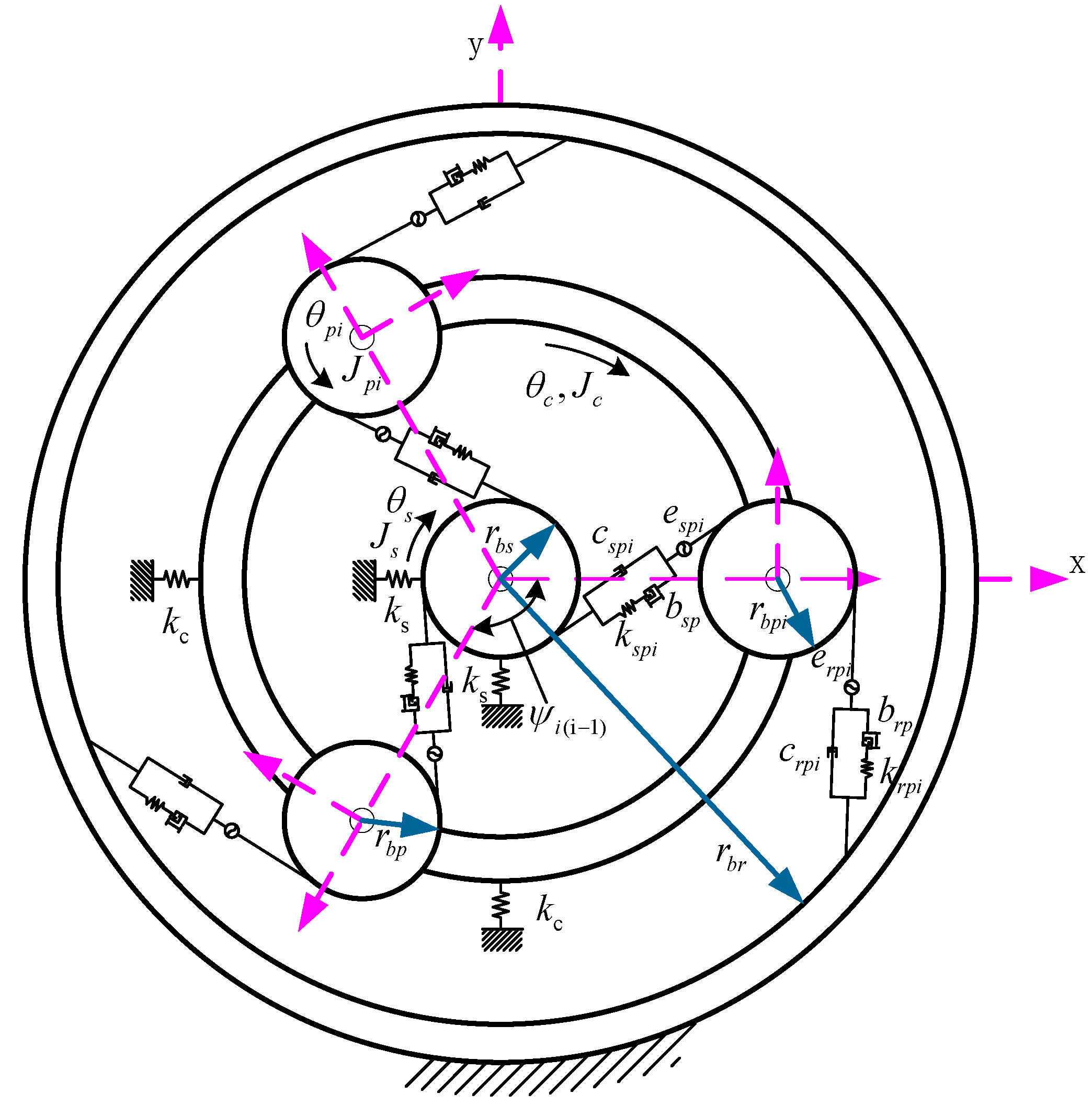
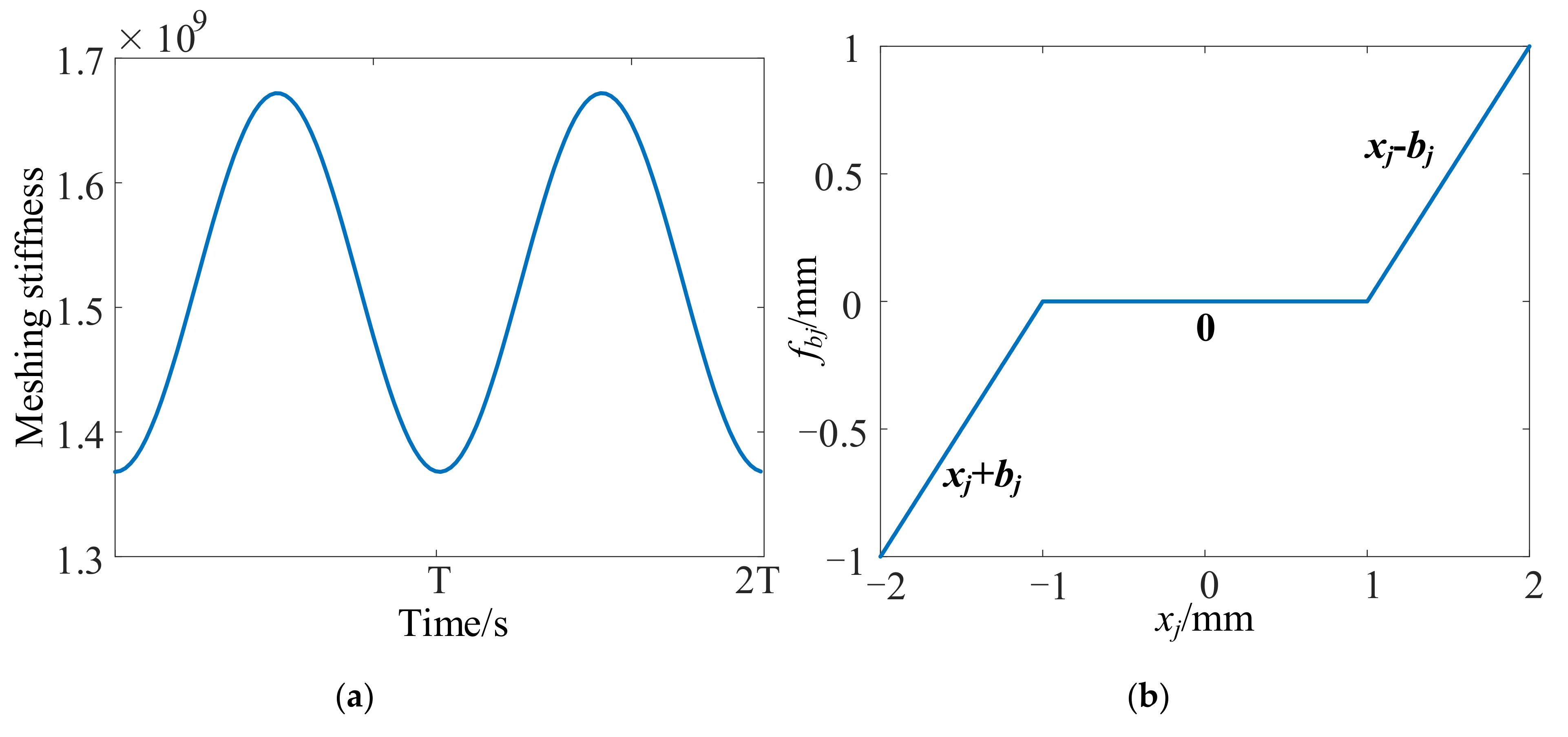
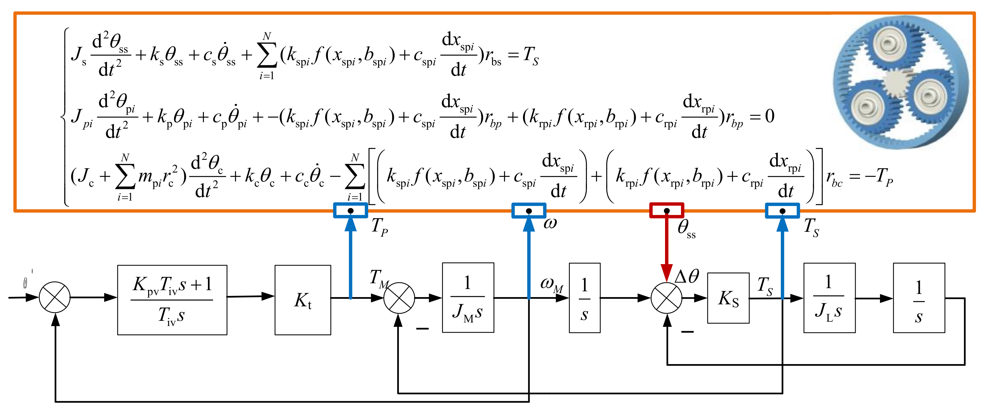
2. Dynamic Modeling of Flexible Joint Considering Gear Angle Error and Friction Torque

The robot joint servo system is composed of servo motor, deceleration components, transmission shafts, loads, etc. Gears are widely used in servo systems, which play a role in changing the transmission direction and adjusting the output speed of the motor. Due to the existence of factors such as backlash and time-varying meshing stiffness, a certain vibration of gear system will be generated when the gear is running, resulting in vibration displacement and affecting the operation of the motor and the load end. There is a certain torsional stiffness in the transmission shaft system and deceleration components, so there is a certain torsional deformation in the robot joint servo system as well. The joint considering torsional deformation is called the flexible joint, and it can be equivalent to a double inertia system. One end of the double inertia system is called the motor end and the other end is called the load end. The motor end and the load end are connected by a torsion spring. The model diagram of the flexible joint servo system is shown in Figure 1. The flow chart of dynamic model analysis is shown in Figure 2.

In Figure 1, $T_a$ represents the driving torque, ${\theta }_m$ represents the motor end angle, ${\theta }_l$ represents the load end angle, $F$ represents the friction torque, $K_s$ represents the torsional stiffness, $J_m$ represents the moment of inertia at the motor end, and $J_l$ represents the moment of inertia at the load end.

In addition, the load is subjected to friction torque during rotation. The models describing the friction torque in the servo system mainly include the LuGre model, the Coulomb model, and the Stribeck model. According to reference [24], different friction models are introduced. It can be seen that an approach for modeling systems with lubrication is the Stribeck friction model. In this paper, friction comes from the transmission system or coupling, etc., which contains lubrication. Therefore, the Stribeck model is adopted. The Stribeck model considers friction torque as a function of speed. The expression of the Stribeck model is shown in Equation (1).

$$F=g\left({\dot{\theta }}_l\right)\frac{{\dot{\theta }}_l}{\left|{\dot{\theta }}_l\right|}+{\sigma }_1{\dot{\theta }}_l=g\left({\dot{\theta }}_l\right)\mathrm{sgn}\left({\dot{\theta }}_l\right)+{\sigma }_1{\dot{\theta }}_l$$

(1)

where ${\sigma }_1$ represents the viscous friction coefficient, and $g\left({\dot{\theta }}_l\right)$ is related to the Stribeck model, as shown in Equation (2).

$$g\left({\dot{\theta }}_l\right)=M_c+\left(M_s-M_c\right)\exp \left[-{\left|\frac{{\dot{\theta }}_l}{{\theta }_s}\right|}^2\right]$$

(2)

where $M_c$ represents the Coulomb friction torque, $M_s$ represents the static friction torque, ${\theta }_s$ represents the friction speed.

The dynamic equation of the flexible joint considering the gear rotation angle error and the friction torque can be obtained according to the transmission relationship as shown in Equation (3).

$$\left\{\begin{array}{l}{J}_m{\ddot{\theta }}_m-K_s\left({\theta }_l-\left({\theta }_m+\Delta \theta \right)\right)=T_a\\ J_l{\ddot{\theta }}_l+K_s\left({\theta }_l-\left({\theta }_m+\Delta \theta \right)\right)=F\end{array}\right.$$

(3)

where $\Delta \theta$ represents the rotation angle error caused by the gear, which can be calculated by Equation (4). The planetary gear reducer is input from the planet carrier, and the sun gear is output, that is, $\Delta \theta ={\theta }_{ss}$. Considering the meshing stiffness, damping, and backlash of the gear system, the dynamic model of the planetary gear system is established by Lagrange method [25,26] as shown in Equation (4). ${\theta }_{ss}$, $J_s$ and $r_{bs}$ are the vibration angular displacement, the moment of inertia and the base circle radius of the sun gear, respectively. ${\theta }_{pi}$, $J_{pi}$, $m_{pi}$ and $r_{bpi}$ are the vibration angular displacement, the moment of inertia, the mass and the base circle radius of the planetary gear, respectively. ${\theta }_c$, $J_c$ and $r_{bc}$ are the vibration angular displacement, the moment of inertia and the radius of the planet carrier, respectively. $e_{spi}$, $b_{spi}$, $c_{spi}$ and $k_{spi}$ are the transmission error, the backlash, the damping and the stiffness of the meshing position of the sun gear and the planet gear, respectively. $e_{rpi}$, $b_{rpi}$, $c_{rpi}$ and $k_{rpi}$ are the transmission error, the gear backlash, the damping and the stiffness of the meshing part of the ring gear and the planetary gear, respectively.

$$\left\{\begin{array}{l}{J}_{\mathrm{s}}\frac{{\mathrm{d}}^2{\theta }_{\mathrm{ss}}}{\mathrm{d}{t}^2}+k_{\mathrm{s}}{\theta }_{\mathrm{ss}}+c_{\mathrm{s}}{\dot{\theta }}_{\mathrm{ss}}+{\displaystyle \sum _{i=1}^N(k_{\mathrm{sp}i}f(x_{\mathrm{sp}i},b_{\mathrm{sp}i})+c_{\mathrm{sp}i}\frac{\mathrm{d}{x}_{\mathrm{sp}i}}{\mathrm{d}t})r_{\mathrm{bs}}}=T_S\\ J_{pi}\frac{{\mathrm{d}}^2{\theta }_{\mathrm{p}i}}{\mathrm{d}{t}^2}+k_{\mathrm{p}}{\theta }_{\mathrm{p}i}+c_{\mathrm{p}}{\dot{\theta }}_{\mathrm{p}i}+-(k_{\mathrm{sp}i}f(x_{\mathrm{sp}i},b_{\mathrm{sp}i})+c_{\mathrm{sp}i}\frac{\mathrm{d}{x}_{\mathrm{sp}i}}{\mathrm{d}t})r_{bp}+(k_{\mathrm{rp}i}f(x_{\mathrm{rp}i},b_{\mathrm{rp}i})+c_{\mathrm{rp}i}\frac{\mathrm{d}{x}_{\mathrm{rp}i}}{\mathrm{d}t})r_{bp}=0\\ (J_{\mathrm{c}}+{\displaystyle \sum _{i=1}^N{m}_{\mathrm{p}i}{r}_{\mathrm{c}}^2})\frac{{\mathrm{d}}^2{\theta }_{\mathrm{c}}}{\mathrm{d}{t}^2}+k_{\mathrm{c}}{\theta }_{\mathrm{c}}+c_{\mathrm{c}}{\dot{\theta }}_{\mathrm{c}}-{\displaystyle \sum _{i=1}^N\left[\left(k_{\mathrm{sp}i}f(x_{\mathrm{sp}i},b_{\mathrm{sp}i})+c_{\mathrm{sp}i}\frac{\mathrm{d}{x}_{\mathrm{sp}i}}{\mathrm{d}t}\right)+\left(k_{\mathrm{rp}i}f(x_{\mathrm{rp}i},b_{\mathrm{rp}i})+c_{\mathrm{rp}i}\frac{\mathrm{d}{x}_{\mathrm{rp}i}}{\mathrm{d}t}\right)\right]r_{bc}}=-T_P\end{array}\right.$$

(4)

where $k_{\mathrm{s}}$, $k_{\mathrm{p}}$, and $k_{\mathrm{c}}$ are the supporting stiffnesses of the sun gear, the planetary gear, and the ring gear, respectively, and $c_{\mathrm{s}}$, $c_{\mathrm{p}}$ and $c_{\mathrm{c}}$ are the supporting damping of the sun gear, the planetary gear, and the ring gear, respectively.

In order to eliminate the influence of rigid body displacement and indefinite solution on the planetary gear system as shown in Figure 3, the Equation (4) is rewritten, and the dynamic transmission error is introduced as shown in Equation (5).

$$\left\{\begin{array}{l}{x}_{\mathrm{sp}i}=r_{\mathrm{bs}}{\theta }_{\mathrm{s}}-r_{\mathrm{bp}i}{\theta }_{\mathrm{p}i}-r_{\mathrm{c}}\cos \alpha {\theta }_{\mathrm{c}}-e_{\mathrm{sp}i}(t)\\ x_{\mathrm{rp}i}=r_{\mathrm{bp}i}{\theta }_{\mathrm{p}i}-r_{\mathrm{c}}\cos \alpha {\theta }_{\mathrm{c}}-e_{\mathrm{rp}i}(t)\end{array}\right.$$

(5)

where the stiffness and the static transmission error are in the form of finite harmonics, and the backlash is in the form of a piecewise function proposed by Kahraman [27], as shown in Equations (6)–(8).

$$\left\{\begin{array}{l}{k}_{\mathrm{sp}i}(t)=k_{\mathrm{hsp}}+k_{\mathrm{asp}}\cos (\omega t+\phi )\\ k_{\mathrm{rp}i}(t)=k_{\mathrm{hrp}}+k_{\mathrm{arp}}\cos (\omega t+\phi )\end{array}\right.$$

(6)

$$\left\{\begin{array}{l}{e}_{\mathrm{sp}i}(t)=e_{\mathrm{asp}}+e_{\mathrm{rsp}}\cos (\omega t+{\phi }_{\mathrm{e}})\\ e_{\mathrm{rp}i}(t)=e_{\mathrm{arp}}+e_{\mathrm{rrp}}\cos (\omega t+{\phi }_{\mathrm{e}})\end{array}\right.$$

(7)

$$f_{bj}=\left\{\begin{array}{c}{x}_j-b_j\\ 0\\ x_j+b_j\end{array}\right.\begin{array}{c}{x}_j>b_j\\ \left|x_j\right|\le b_j\\ x_j<-b_j\end{array}$$

(8)

where the meshing of the sun gear and the planetary gear is called the internal meshing, the meshing of the planetary gear and the ring gear is called the external meshing, $k_{hsp}$ and $k_{hrp}$ are the mean stiffnesses of internal and external meshing, respectively, $k_{asp}$ and $k_{arp}$ are the stiffness amplitudes of internal and external meshing, respectively, $e_{asp}$ and $e_{arp}$ are the mean static transmission errors of internal and external meshing, respectively, and $e_{rsp}$ and $e_{rrp}$ are the static transmission error amplitudes of internal and external meshing, respectively. In Equation (8), j (j = spi and rpi) represents the backlash of internal and external meshing, respectively.

A schematic diagram of stiffness and backlash of the gear system can be obtained as shown in Figure 4. In Figure 4a, $T$ represents a meshing cycle of the gear.

According to Equation (3), the dynamic equation considering gear angle error and friction model is a nonlinear equation, which brings difficulties to the design of servo system controller parameters. The influence of gear system and system friction torque is introduced into the double inertia system as the interference term of the system, which also belongs to the modeling error of the system. It is relatively smaller than load feedback and has no effect on the determination of PI parameters. In order to determine the controller parameters for the subsequent application of the pole assignment strategy, the influence of the gear angle error and the friction torque are ignored. After ignoring the nonlinear factors such as gear angle error and friction torque, the dynamic equation of the flexible joint servo system can be obtained as shown in Equation (9).

$$\left\{\begin{array}{l}{J}_m{\ddot{\theta }}_m-K_s\left({\theta }_l-{\theta }_m\right)=T_a\\ J_l{\ddot{\theta }}_l+K_s\left({\theta }_l-{\theta }_m\right)=0\end{array}\right.$$

(9)

According to Equation (9), the state space equation of the flexible joint can be obtained as shown in Equation (10).

$$\left[\begin{array}{c}{\dot{\theta }}_m\\ {\ddot{\theta }}_m\\ {\dot{\theta }}_l\\ {\ddot{\theta }}_l\end{array}\right]=\left[\begin{array}{cccc}0& 1& 0& 0\\ -\frac{K_s}{J_m}& 0& \frac{K_s}{J_m}& 0\\ 0& 0& 0& 1\\ \frac{K_s}{J_l}& 0& -\frac{K_s}{J_l}& 0\end{array}\right]\left[\begin{array}{c}{\theta }_m\\ {\dot{\theta }}_m\\ {\theta }_l\\ {\dot{\theta }}_l\end{array}\right]+\left[\begin{array}{cccc}0& 0& 0& 0\\ \frac{1}{J_m}& 0& 0& 0\\ 0& 0& 0& 0\\ 0& -\frac{1}{J_l}& 0& 0\end{array}\right]\left[\begin{array}{c}{T}_a\\ 0\\ 0\\ 0\end{array}\right]$$

(10)

According to Equation (10), the transfer function from the output speed of the motor to the driving torque can be obtained as shown in Equation (11).

$$\frac{{\dot{\theta }}_m}{T_a}=\frac{J_l{s}^2+K_s}{J_m{J}_l{s}^3+\left(J_m+J_l\right)K_{s}s}$$

(11)

We can represent Equation (11) in the form as shown in Equation (12).

$$\frac{{\dot{\theta }}_m}{T_a}=\frac{s^2+{\omega }_a^2}{J_m{s}^3+J_m{\omega }_n^{2}s}$$

(12)

where ${\omega }_a$ represents the anti-resonant frequency and ${\omega }_n$ represents the resonant frequency, and their expressions are shown in Equations (13) and (14).

$${\omega }_a=\sqrt{\frac{K_s}{J_l}}$$

(13)

$${\omega }_n={\omega }_a\sqrt{1+R}$$

(14)

In Equation (14), R represents the ratio of inertia between the load end and the motor end, and its expression is shown in Equation (15).

$$R=\frac{J_l}{J_m}$$

(15)

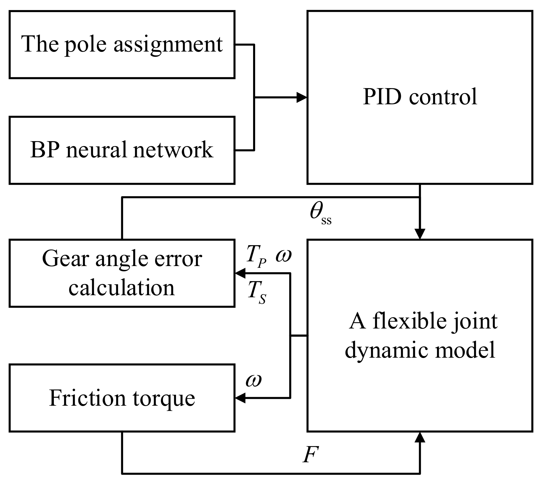
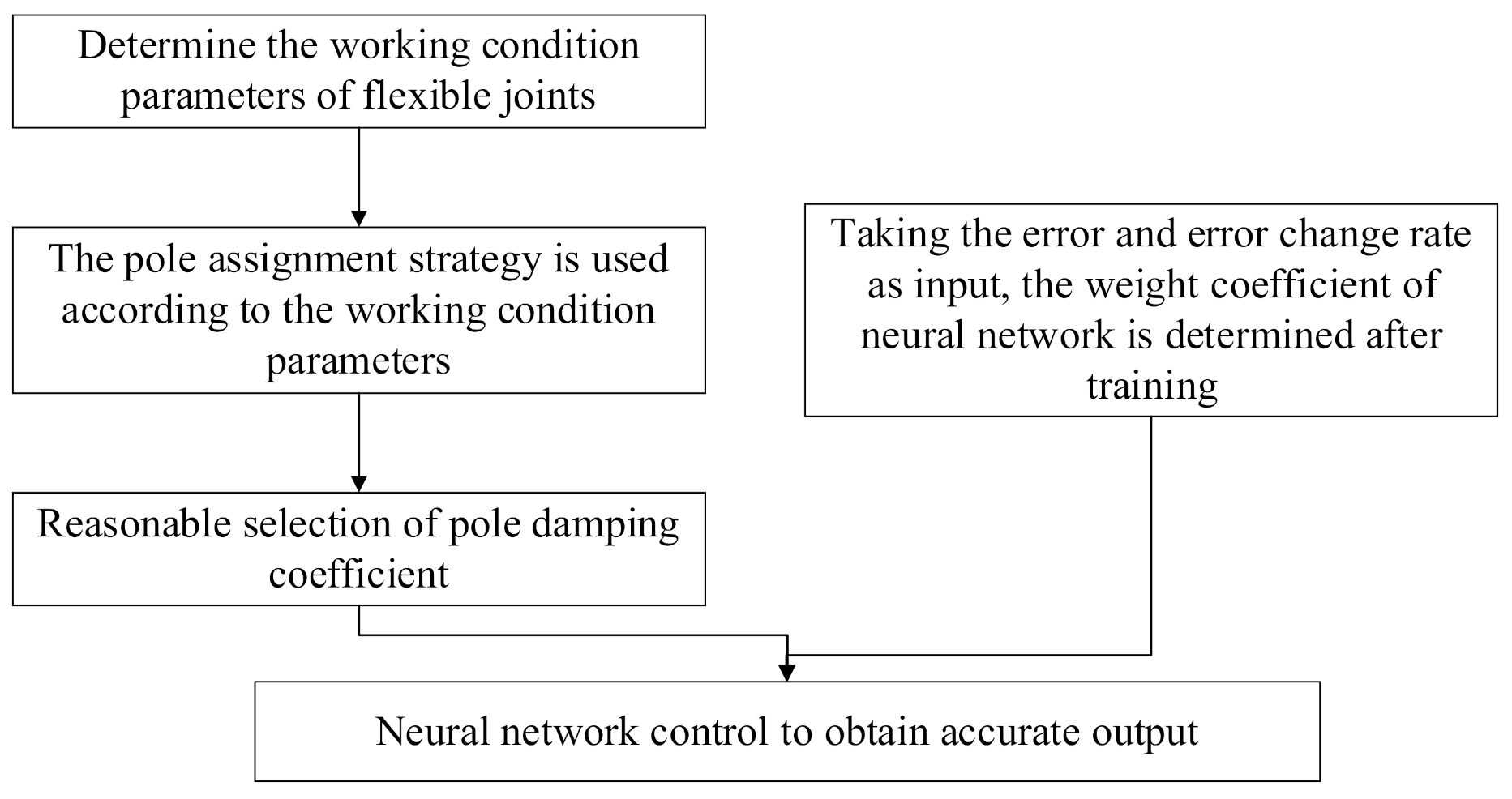
3. Joint Control Strategy Based on BP Neural Network and Pole Placement Method

The control strategy of the flexible joint servo system mostly adopts a three-loop control strategy, which contains current loop, speed loop and displacement loop. It can be known that the current loop and the speed loop have a larger bandwidth. The influence of the current loop can be ignored during the speed loop control strategy. This paper mainly studies the speed control of the flexible joint, so the influence of position loop is not considered. The output speed of the motor is easy to measure, so the speed of the motor is used as the feedback signal. Through the closed-loop control of the motor speed, the control of the output speed of the load is indirectly realized.

The PI control strategy is widely used in the speed control strategy of the servo system. Therefore, this paper uses PI control strategy to control the speed loop of the servo system. The control block diagram of the flexible joint servo system is shown in Figure 5.

The controller parameters play a key role in whether the flexible joint servo system can obtain stable speed output. Therefore, it is necessary to design the controller parameters according to the controlled object. In this paper, the pole assignment strategy is used to design controller parameters.

The moment of inertia of the load of the servo system in the mechanical arm flexible joint has obvious time-varying characteristics. It is difficult to obtain a stable control effect if the controller parameters are fixed. With the development of intelligent control, fuzzy logic systems and neural networks provide theoretical possibilities for changing controller parameters in real time. Compared with the PI controller with fixed parameters, the PI controller that can change parameters in real time can obtain more accurate control effects. Therefore, this paper uses the BP neural network to adjust the controller parameters in real time according to the error and the change rate of error. It is necessary to roughly determine the control parameters before using the BP neural network. In this paper, the pole assignment strategy is used to roughly determine the control parameters, and then the BP neural network is used to fine tune the controller parameters. The specific control flow is shown in Figure 6.

3.1. Controller Parameters Tuning Based on Pole Assignment

According to reference [15], the appropriate controller parameters are roughly determined by using the pole assignment strategy, which is ready for the next step of using the BP neural network. According to Equation (12), the closed-loop transfer function of the flexible joint servo system can be obtained as shown in Equation (16).

$$\frac{{\dot{\theta }}_m\left(s\right)}{{\dot{\theta }}^{\ast }\left(s\right)}=\frac{\left(K_{P}s+K_I\right)\left(s^2+{\omega }_a^2\right)}{J_m{s}^2\left(s^2+{\omega }_n^2\right)+\left(K_{P}s+K_I\right)\left(s^2+{\omega }_a^2\right)}$$

(16)

where ${\theta }^{\ast }$ represents the rated input angle, $K_p$ represents the proportional parameter of the controller, $K_I$ represents the integral parameter of the controller. We can represent the denominator of Equation (16) in the form of Equation (17).

$$\left\{\begin{array}{l}{J}_m{s}^2\left(s^2+{\omega }_n^2\right)+\left(K_{P}s+K_I\right)\left(s^2+{\omega }_a^2\right)=J_{m}M\\ M=\left(s^2+2{\xi }_{a1}{\omega }_{a1}s+{\omega }_{a1}^2\right)\left(s^2+2{\xi }_{b1}{\omega }_{b1}s+{\omega }_{b1}^2\right)\end{array}\right.$$

(17)

where ${\omega }_{a1}$ and ${\omega }_{b1}$ represent the natural frequencies of the pole; ${\xi }_{a1}$ and ${\xi }_{b1}$ represent the pole damping coefficient.

According to the equivalence of corresponding terms, Equation (18) holds.

$$\left\{\begin{array}{l}{K}_P=J_m\left(2{\xi }_{a1}{\omega }_{a1}+2{\xi }_{b1}{\omega }_{b1}\right)\\ K_I=\frac{J_m{\omega }_{a1}^2{\omega }_{b1}^2}{{\omega }_a^2}\\ {\omega }_{a1}^2+{\omega }_{b1}^2+4{\xi }_{a1}{\xi }_{b1}{\omega }_{a1}{\omega }_{b1}={\omega }_n^2+\frac{{\omega }_{a1}^2{\omega }_{b1}^2}{{\omega }_a^2}\\ {\xi }_{a1}{\omega }_{a1}{\omega }_{b1}^2+{\xi }_{b1}{\omega }_{b1}{\omega }_{a1}^2=\left({\xi }_{a1}{\omega }_{a1}+{\xi }_{b1}{\omega }_{b1}\right){\omega }_a^2\end{array}\right.$$

(18)

According to references [15,23], there are three different pole assignment strategies, which are the same amplitude, the same real part and the same damping coefficient. In this paper, the pole assignment method with the same amplitude is selected to design the controller parameters. The so-called pole assignment strategy with the same amplitude means that the poles have the same radius. Therefore, substituting ${\omega }_{a1}={\omega }_{b1}$ into Equation (18), Equation (19) can be obtained.

$$\left\{\begin{array}{l}{\omega }_{a1}={\omega }_{b1}={\omega }_a\\ {\xi }_{a1}{\xi }_{b1}=\frac{R}{4}\\ K_P=2J_m{\omega }_a\left({\xi }_{a1}+{\xi }_{b1}\right)\\ K_I=J_m{\omega }_a^2\end{array}\right.$$

(19)

According to Equation (19), the expression of controller parameters can be obtained. Therefore, the controller parameters can be adjusted by changing the pole damping coefficient.

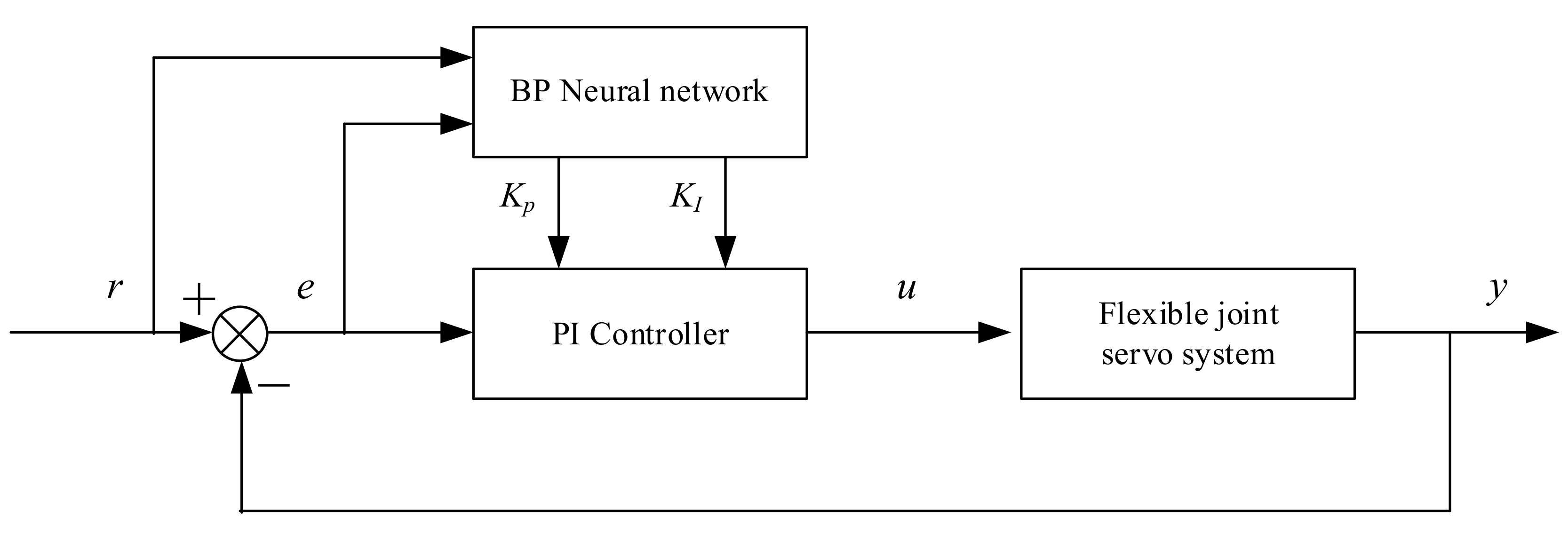
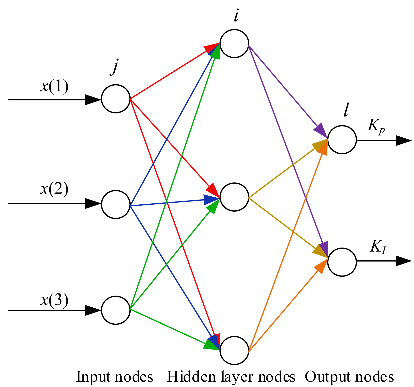
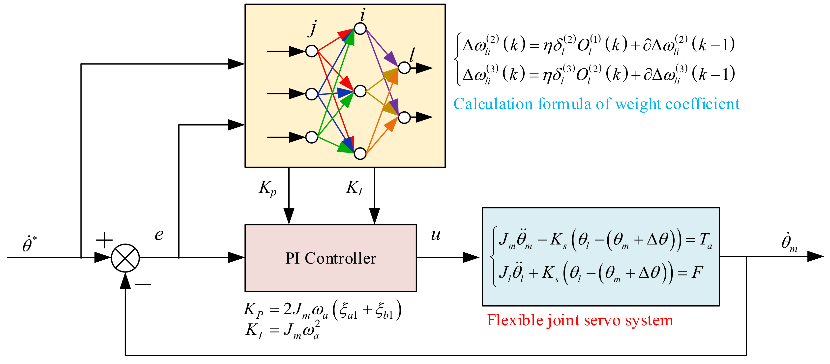
3.2. Controller Parameters Tuning Based on BP Neural Network

Neural network has the ability to approximate any nonlinear function and can realize the PI control strategy of the optimal controller parameter combination by learning the system performance. The BP neural network adjusts the PI controller parameters according to the operating state, and then achieves the optimization of a certain performance index. The PI controller using BP neural network is shown in Figure 7.

According to Figure 7, the output state of the neurons in the output layer corresponds to the proportional and integral parameters of the PI controller. Through the self-learning of the neural network and the adjustment of the weighting coefficient, its stable state corresponds to a certain optimal controller parameter. The BP neural network in Figure 7 adopts a three-layer structure, one input layer, one hidden layer and one output layer. The structure of the BP neural network is shown in Figure 8.

In Figure 8, $j$ represents an input layer node, $i$ represents a hidden layer node, and $l$ represents an output layer node. The input layer has m input nodes, the hidden layer has q hidden nodes, and the output layer has two output nodes.

The input node corresponds to the selected system operating state quantity, such as rated input, system output, error, etc. The output nodes correspond to the proportional parameter and integral parameter in the PI controller. Since the controller parameters cannot be negative, the neuron activation function of the output layer takes a non-negative Sigmoid function.

It can be seen from Figure 8 that the output of the input layer of the BP neural network is shown in Equation (20).

$$O_j^{(i)}=x\left(j\right),\begin{array}{cc}& j=1,2,3,\cdots ,m\end{array}$$

(20)

The input of the hidden layer is shown in Equation (21).

$${\mathrm{net}}_i^{\left(2\right)}\left(k\right)={\displaystyle \sum _{j=0}^m{\omega }_{ij}^{\left(2\right)}}{O}_j^{\left(1\right)}$$

(21)

where ${\omega }_{ij}^{\left(2\right)}$ represents the weighting coefficient from the input layer to the hidden layer.

The output of the hidden layer is shown in Equation (22).

$$O_j^{(2)}\left(k\right)=g\left({\mathrm{net}}_i^{\left(2\right)}\left(k\right)\right),\begin{array}{cc}& i=1,2,3,\cdots ,q\end{array}$$

(22)

where $g(x)$ represents the positive and negative symmetric Sigmoid function, and its expression is shown in Equation (23).

$$g\left(x\right)=\tanh \left(x\right)=\frac{e^x-e^{-x}}{e^x+e^{-x}}$$

(23)

The input of the two nodes in the output layer of the neural network is shown in Equation (24).

$${\mathrm{net}}_l^{\left(3\right)}\left(k\right)={\displaystyle \sum _{i=0}^q{\omega }_{li}^{\left(3\right)}}{O}_i^{\left(2\right)}\left(k\right)$$

(24)

where ${\omega }_{li}^{\left(3\right)}$ represents the weighting coefficient from the hidden layer to the output layer.

Thus, two outputs of the output layer can be obtained as shown in Equation (25).

$$O_l^{(3)}\left(k\right)=f\left({\mathrm{net}}_l^{\left(3\right)}\left(k\right)\right),\begin{array}{cc}& l=1,2\end{array}$$

(25)

where $f(x)$ represents the neuron activation function of the output layer, and its expression is shown in Equation (26).

$$f\left(x\right)=\frac{1}{2}\left(1+\tanh \left(x\right)\right)=\frac{e^x}{e^x+e^{-x}}$$

(26)

The two outputs of the output layer of the BP neural network are the PI controller parameters as shown in Equation (27).

$$\left\{\begin{array}{l}{O}_1^{(3)}\left(k\right)=K_P\\ O_2^{(3)}\left(k\right)=K_I\end{array}\right.$$

(27)

The performance index function selected in this paper is shown in Equation (28).

$$\left\{\begin{array}{l}E\left(k\right)=\frac{1}{2}{\left(r\left(k\right)-y\left(k\right)\right)}^2\\ {\dot{\theta }}^{\ast }\left(k\right)=r\left(k\right)\\ {\dot{\theta }}_m\left(k\right)=y\left(k\right)\end{array}\right.$$

(28)

where, r(k) represents the input node, which is the state quantity of system operation, and y(k) is the output node. The difference of them represents the error. In this paper, r(k) is the expected value of motor speed, and y(k) is the actual motor speed.

The gradient descent algorithm is used to modify the weight coefficient of the BP neural network, and its expression is shown in Equation (29).

$$\Delta {\omega }_{li}^{\left(3\right)}\left(k\right)=-\eta \frac{\partial E\left(k\right)}{\partial {\omega }_{li}^{\left(3\right)}}+\partial \Delta {\omega }_{li}^{\left(3\right)}\left(k-1\right)$$

(29)

where $\eta$ represents the learning rate, $\partial$ represents the inertia coefficient, which is used to make the contraction converge to the global minimum quickly.

According to Equation (29), Equation (30) can be obtained.

$$\frac{\partial E\left(k\right)}{\partial {\omega }_{li}^{\left(3\right)}}=\frac{\partial E\left(k\right)}{\partial y\left(k\right)}·\frac{\partial y\left(k\right)}{\partial u\left(k\right)}·\frac{\partial u\left(k\right)}{\partial O_l^{\left(3\right)}\left(k\right)}·\frac{\partial O_l^{\left(3\right)}\left(k\right)}{\partial {\mathrm{net}}_l^{\left(3\right)}\left(k\right)}·\frac{\partial {\mathrm{net}}_l^{\left(3\right)}\left(k\right)}{\partial {\omega }_{ll}^{\left(3\right)}\left(k\right)}$$

(30)

Due to the non-linear factors of the flexible joint servo system model, it is difficult to obtain $\partial y\left(k\right)/\partial u\left(k\right)$. We can use Equation (31) as an approximation of $\partial y\left(k\right)/\partial u\left(k\right)$.

$$\frac{\partial y\left(k\right)}{\partial u\left(k\right)}\approx \frac{y\left(k\right)-y\left(k-1\right)}{u\left(k\right)-u\left(k-1\right)}$$

(31)

Since $u(k)$ and $u\left(k-1\right)$ are very close, it is easy to cause the infinite phenomenon in Equation (31). Therefore, this paper uses Equation (32) instead of Equation (31).

$$\frac{\partial y\left(k\right)}{\partial u\left(k\right)}\approx \mathrm{sgn}\left(\frac{y\left(k\right)-y\left(k-1\right)}{u\left(k\right)-u\left(k-1\right)}\right)$$

(32)

According to the classical incremental numerical PID control algorithm, the expression $u\left(k\right)$ can be obtained as shown in Equation (33).

$$u\left(k\right)=u\left(k-1\right)+K_p\left(e\left(k\right)-e\left(k-1\right)\right)+K_{I}e\left(k\right)$$

(33)

According to Equation (27), Equation (33) can be written in the form of Equation (34).

$$u\left(k\right)=u\left(k-1\right)+O_1^{(3)}\left(e\left(k\right)-e\left(k-1\right)\right)+O_2^{(3)}e\left(k\right)$$

(34)

According to Equation (34), Equation (35) can be obtained.

$$\left\{\begin{array}{l}\frac{\partial u\left(k\right)}{\partial O_1^{\left(3\right)}\left(k\right)}=e\left(k\right)-e\left(k-1\right)\\ \frac{\partial u\left(k\right)}{\partial O_2^{\left(3\right)}\left(k\right)}=e\left(k\right)\end{array}\right.$$

(35)

According to Equations (33) and (35), the weight calculation formula of the output layer of the BP neural network can be obtained as shown in Equation (36).

$$\Delta {\omega }_{li}^{\left(3\right)}\left(k\right)=-\eta e\left(k\right)\frac{\partial y\left(k\right)}{\partial u\left(k\right)}\frac{\partial u\left(k\right)}{\partial O_l^{\left(3\right)}\left(k\right)}{f}^{\prime }\left({\mathrm{net}}_l^{\left(3\right)}\left(k\right)O_l^{\left(2\right)}\left(k\right)+\partial \Delta {\omega }_{li}^{\left(3\right)}\left(k-1\right)\right)$$

(36)

Substituting Equation (32) into Equation (36), and then Equation (37) holds.

$$\Delta {\omega }_{li}^{\left(3\right)}\left(k\right)=-\eta e\left(k\right)\mathrm{sgn}\left(\frac{y\left(k\right)-y\left(k-1\right)}{u\left(k\right)-u\left(k-1\right)}\right)\frac{\partial u\left(k\right)}{\partial O_l^{\left(3\right)}\left(k\right)}{f}^{\prime }\left({\mathrm{net}}_l^{\left(3\right)}\left(k\right)\right)O_l^{\left(2\right)}\left(k\right)+\partial \Delta {\omega }_{li}^{\left(3\right)}\left(k-1\right)$$

(37)

In order to simplify Equation (37), Equation (38) holds.

$${\delta }_l^{\left(3\right)}=e\left(k\right)\mathrm{sgn}\left(\frac{y\left(k\right)-y\left(k-1\right)}{u\left(k\right)-u\left(k-1\right)}\right)\frac{\partial u\left(k\right)}{\partial O_l^{\left(3\right)}\left(k\right)}{f}^{\prime }\left({\mathrm{net}}_l^{\left(3\right)}\left(k\right)\right)$$

(38)

According to Equation (38), the weight calculation formula of the output layer of the BP neural network can be obtained as shown in Equation (39).

$$\Delta {\omega }_{li}^{\left(3\right)}\left(k\right)=\eta {\delta }_l^{\left(3\right)}{O}_l^{\left(2\right)}\left(k\right)+\partial \Delta {\omega }_{li}^{\left(3\right)}\left(k-1\right)$$

(39)

Similarly, the formula for calculating the weight coefficient of the hidden layer can be obtained as shown in Equation (40).

$$\left\{\begin{array}{l}\Delta {\omega }_{li}^{\left(2\right)}\left(k\right)=\eta {\delta }_l^{\left(2\right)}{O}_l^{\left(1\right)}\left(k\right)+\partial \Delta {\omega }_{li}^{\left(2\right)}\left(k-1\right)\\ {\delta }_l^{\left(2\right)}=g^{\prime }\left({\mathrm{net}}_l^{\left(2\right)}\left(k\right)\right){\displaystyle \sum _{i=1}^2{\delta }_l^{\left(3\right)}{\omega }_{li}^{\left(3\right)}\left(k\right)}\end{array}\right.$$

(40)

The algorithm of PI controller based on BP neural network is shown below.

(1) Determine the structure of the BP neural network, that is, the number of input nodes m, the number of hidden layer nodes q, and the initial values of the weight coefficients of each layer of the neural network are ${\omega }_{li}^{\left(2\right)}\left(0\right)$ and ${\omega }_{li}^{\left(3\right)}\left(0\right)$, and the learning rate $\eta$ and the inertia coefficient $\partial$ are selected.

(2) $r\left(k\right)$ and $y\left(k\right)$ are obtained by sampling, and the time error $e\left(k\right)$ is calculated.

(3) Calculate the input and output values of each layer of the neural network, and adjust the controller parameters.

(4) Calculate $u\left(k\right)$ according to Equation (34).

(5) Carry out neural network learning and adjust the weighting coefficients online according to Equations (39) and (40) to realize the adaptive adjustment of PID parameters.

In summary, this paper adopts a control strategy based on BP neural network and pole assignment method to control the flexible joint servo system. The control block diagram is shown in Figure 9.

4. Numerical Simulation Analysis

In order to verify the effectiveness of the proposed control strategy, the simulation analysis of the flexible joint servo system is carried out based on Matlab and Simulink in this paper. Firstly, the influence of friction torque on the flexible joint servo system is illustrated through simulation analysis. Then the influence of different pole damping coefficient on the output of the servo system is analyzed, and the reasonable interval of the pole damping coefficient is given. Finally, the effectiveness of the proposed control strategy is verified by comparing the output errors of different control strategies.

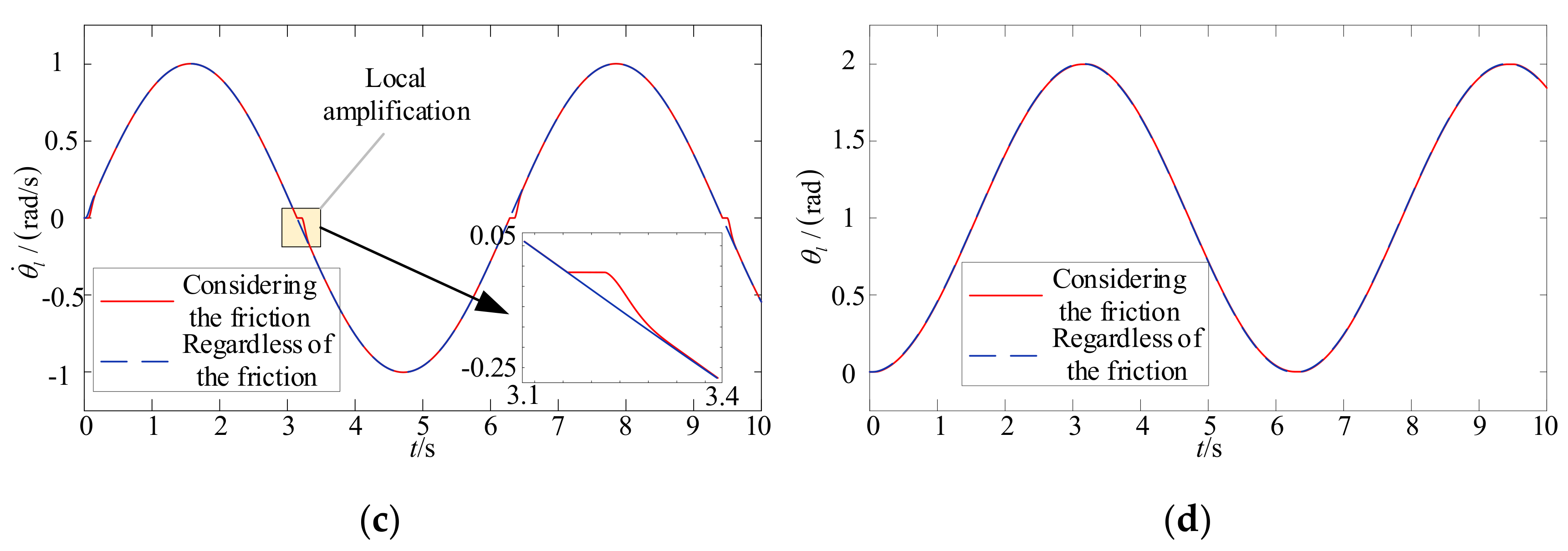
4.1. The Effect of Friction on the System

In the robotic arm flexible joint servo system, the servo motor drives the load to rotate. In the process of load rotation, it is affected by friction. In this paper, the Stribeck model shown in Equation (1) is used to describe the friction torque of the load. In order to analyze the influence of friction torque on the flexible joint servo system, the moment of inertia of the motor end is set to 0.05, the moment of inertia of the load end is set to 0.15, and the torsional stiffness of the joint is set to 300. In the simulation process, a sinusoidal signal is selected as the rated input signal of the motor end. Thus, the law of friction torque changing with time can be obtained as shown in Figure 10a. The influence of friction torque on the input torque required by the servo system is obtained as shown in Figure 10b. The influence of friction torque on the servo system is not only reflected in the required input torque. The friction torque also affects the output of the system speed. The influence of friction torque on the load end speed and rotation angle is shown in Figure 10c,d.

According to Figure 10a, it can be seen that when the friction torque changes in the direction of the speed, a sudden change will occur. This sudden change of friction torque is due to the static friction effect. According to Figure 10b, we can see that the sudden change of the friction torque will cause the sudden change of the required input torque, but the controller cannot provide the required driving torque within a short period of time, which will cause fluctuations in the output speed of the servo system. According to Figure 10c, we can clearly see this speed fluctuation. The speed fluctuation will have a certain effect on the angle of rotation, but according to Figure 10d, it can be seen that this effect is relatively weak.

In summary, the friction torque received by the flexible joint servo system will affect the input torque and load speed. Therefore, the influence of friction torque cannot be ignored for robots with high accuracy.

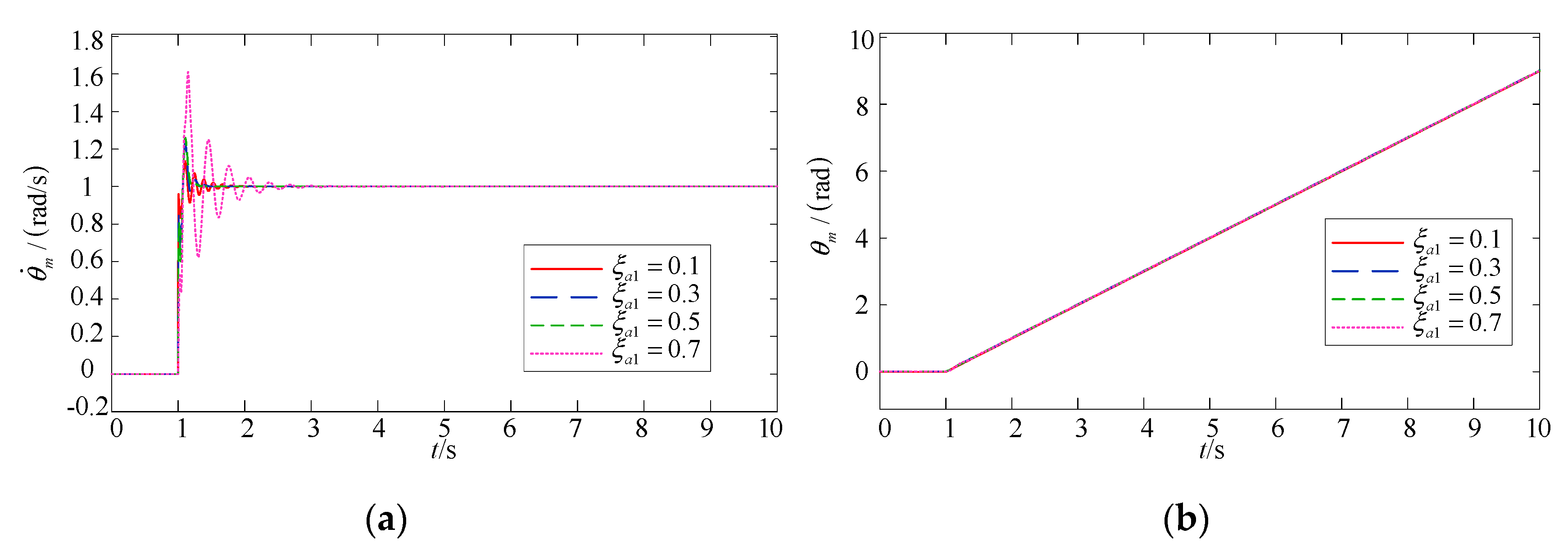
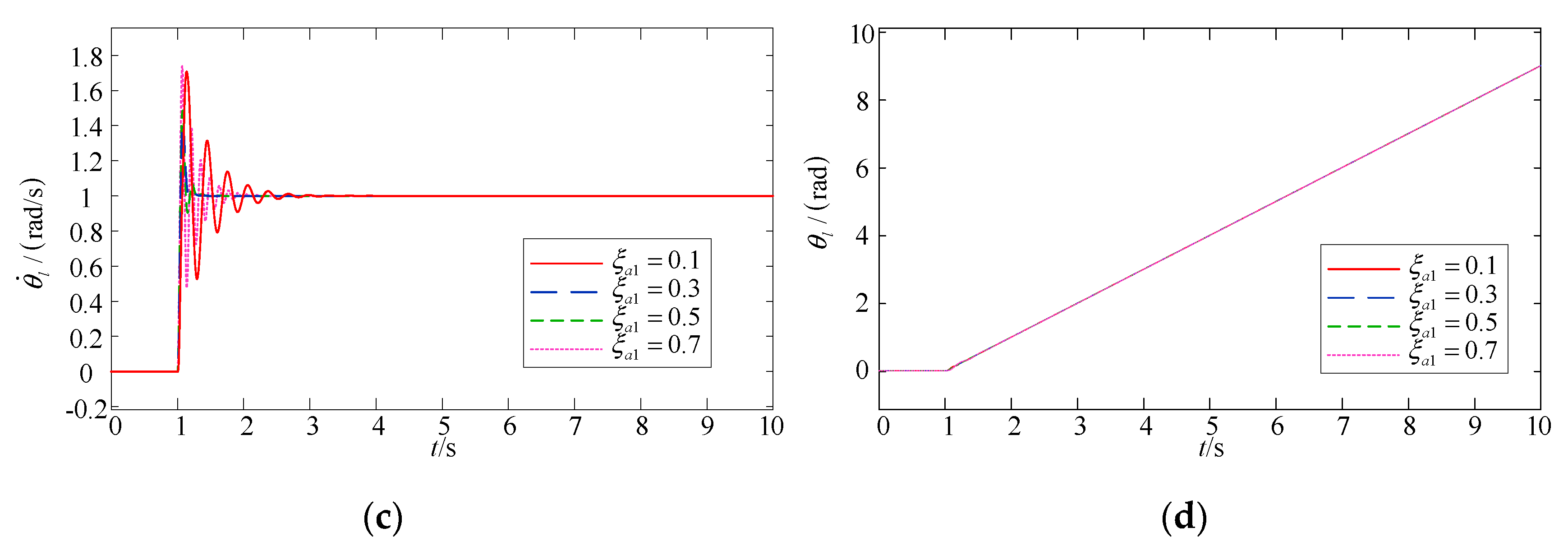
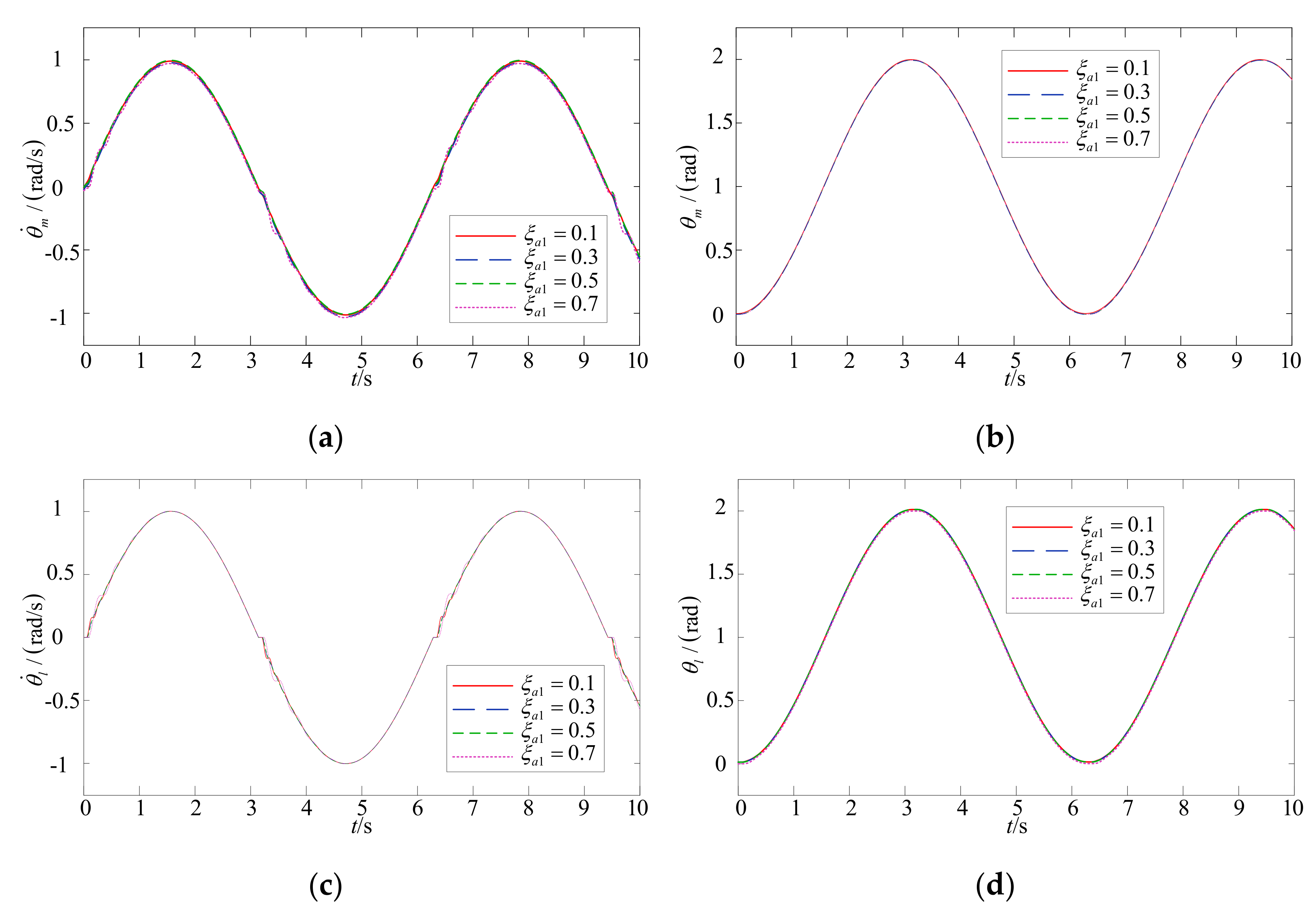
4.2. The Influence of Pole Damping Coefficient on System Output

The selection of the controller parameters plays a crucial role in the control effect of the flexible joint servo system. In this paper, the pole assignment strategy of the same amplitude is used to roughly design the controller parameters. According to Equation (19), it can be seen that the design of the controller parameters can be transformed into the selection of the pole damping coefficient. Different pole damping coefficient will affect the output of the system. In order to clarify the influence of the value of the pole damping coefficient on the output of the system. Within this paper, the moment of inertia at the motor end is set to 0.05, the moment of inertia at the load end is set to 0.15, and the torsional stiffness of the flexible joint is set to 500. In order to illustrate the influence of the pole damping coefficient, the rated signals of the motor speed are set as a step signal and a sinusoidal signal, respectively. Therefore, the output results of different pole damping coefficients at the motor end and load end can be obtained as shown in Figure 11 and Figure 12. Among them, Figure 11 shows the output results under the step signal and Figure 12 shows the output results of the sinusoidal signal.

According to Figure 11 and Figure 12, the value of the pole damping coefficient will affect the fluctuation of the output speed. This phenomenon is especially obvious under the step signal input. However, the value of the pole damping coefficient has a weaker effect on the angle of rotation. According to Figure 11, the value of the pole damping coefficient, whether too large or too small, will aggravate the fluctuation of the output speed. Based on this, it can be obtained that the ideal value range of the pole damping coefficient is 0.3–0.5 through numerical different simulation experiments. In this interval, the design of the PI controller parameters of the flexible joint servo system can obtain a relatively stable output.

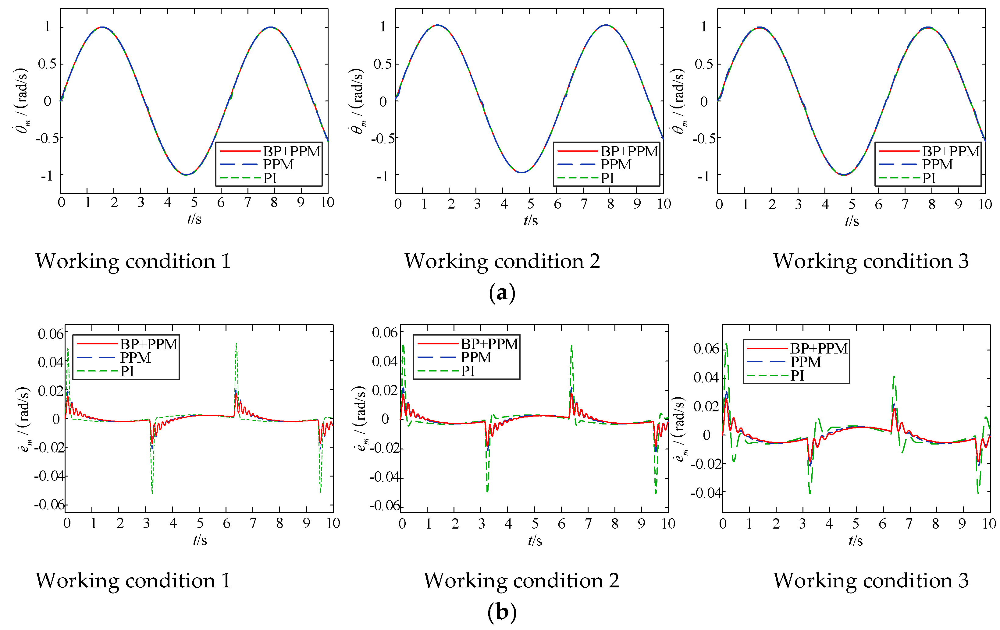
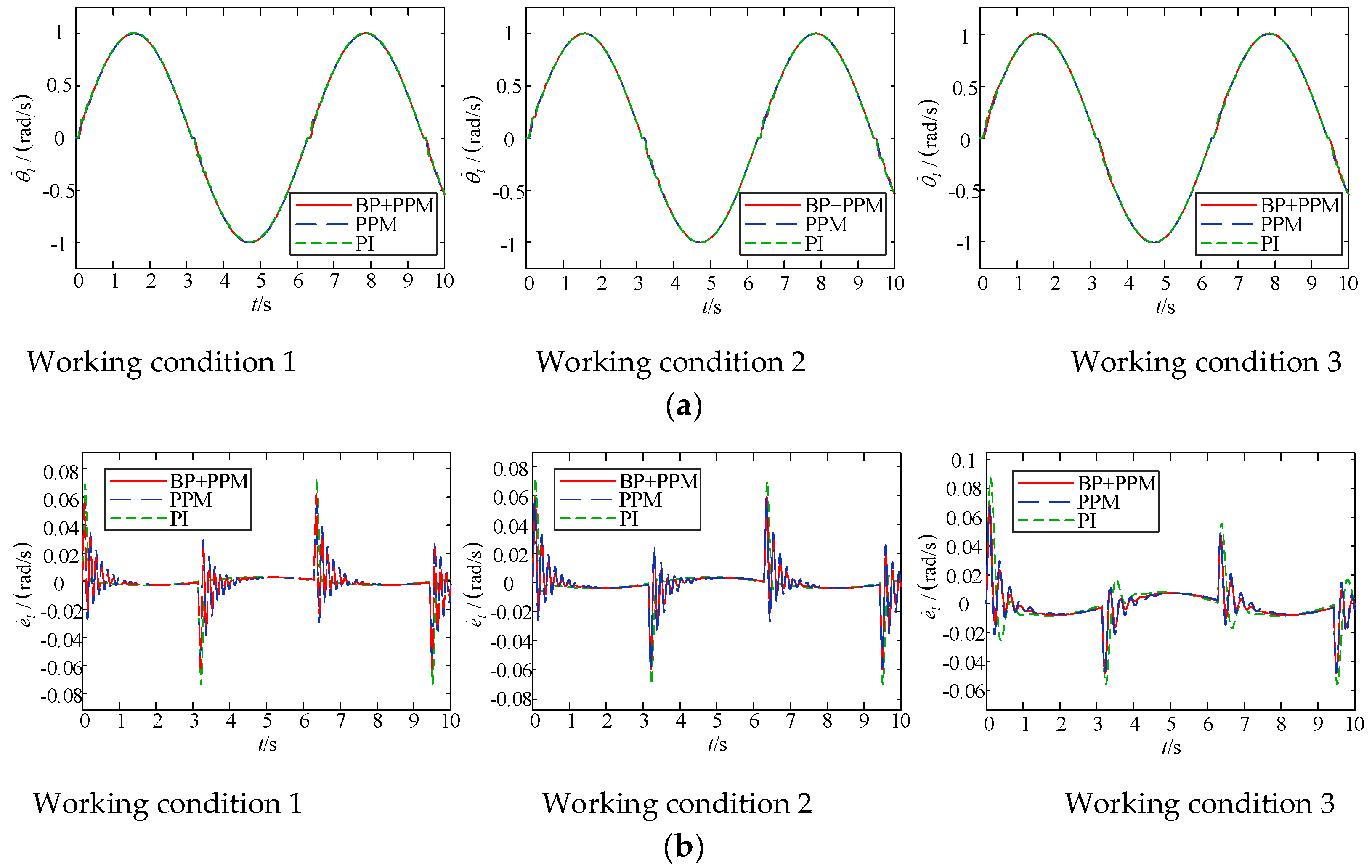
4.3. Joint Control Strategy of BP Neural Network and Pole Assignment

During the movement of the robot, the moment of inertia at the load end of the flexible joint will change. In order to make the robot obtain good output under different working conditions, this paper chooses three different working conditions to carry out simulation experiments. The parameters of the three different working conditions are shown in

Table 1. Parameters of the dual-flexible manipulator.

Parameters	Condition 1	Condition 2	Condition 3
Flexible load inertia Jl/kgm2	0.186	0.256	0.573
Motor inertia Jm/kgm2	0.062	0.062	0.062
Torsional stiffness Ks/Nm/rad	305	305	305
Anti-resonant frequency ωa	40.4943	34.5168	23.0713
Resonant frequency ωn	80.9885	78.1714	73.8352
Inertia ratio	3	4.1290	9.2419
Pole damping coefficient	0.3	0.3	0.3
Controller parameters for pole assignment	14/101	16/73	22/33
Common PI controller parameters	20/80	20/80	20/80

.

In order to verify the effectiveness of the control strategy proposed in this paper, the joint control strategy of BP neural network and pole assignment, the pole assignment control strategy, and the common PI control strategy are respectively selected to control the flexible joint. The three working conditions in Table 1 are selected for simulation, and the simulation results of different control strategies are obtained as shown in Figure 13 and Figure 14. Figure 13a shows the speed output at the motor end, Figure 13b shows the error of the speed output at the motor end. Figure 14a shows the speed output at the load end, Figure 14b shows the speed error at the load end.

According to Figure 13b, taking the maximum error of PI method as the benchmark, the percentage of other methods’ maximum errors to it is obtained.

The method of the joint control strategy of BP neural network and pole assignment in different working conditions: 30% (Working condition 1), 32% (Working condition 2) and 38% (Working condition 3).

The method of the joint control strategy of pole assignment in different working conditions: 40% (Working condition 1), 44% (Working condition 2) and 44% (Working condition 3).

According to Figure 13 and Figure 14, the control strategy proposed in this paper has small error under any working conditions, which shows that the control strategy proposed in this paper can effectively reduce the error and improve the control accuracy.

5. Conclusions

Based on the double inertia system, an integrated joint motor servo system model considering gear angle error and friction interference is established, and a joint control strategy based on BP neural network and pole assignment method is designed to suppress the vibration of the system. The following conclusions can be obtained through simulation analysis:

(1) When the friction torque changes in the direction of the speed, a sudden change will occur. This sudden change of friction torque will affect the input torque, and cause fluctuations in the output speed and the output rotation angle of the servo system.

(2) The pole damping coefficient will affect the fluctuation of the output speed. This phenomenon is especially obvious under the step signal input. In the range 0.3–0.5 of the pole damping coefficient, the design of the PI controller parameters of the flexible joint servo system can obtain a relatively stable output.

(3) The control strategy proposed in this paper has small error under different working conditions, which shows that the control strategy proposed in this paper can effectively reduce the error and improve the control accuracy.

References

1. Li, F.; Li, X.; Guo, Y.; Shang, D. Analysis of Contact Mechanical Characteristics of Flexible Parts in Harmonic Gear Reducer. Shock Vib. 2021, 2021, 5521320. [Google Scholar] [CrossRef]
2. Spong, M.W.; Hutchinson, S.; Vidyasagar, M. Robot Modeling and Control. Ind. Robot. 2006, 17, 709–737. [Google Scholar] [CrossRef]
3. Ma, C.; Cao, J.; Qiao, Y. Polynomial-Method-Based Design of Low-Order Controllers for Two-Mass Systems. IEEE Trans. Ind. Electron. 2013, 60, 969–978. [Google Scholar] [CrossRef]
4. Mirzaei, M.A.; Nazari-Heris, M.; Mohammadi-Ivatloo, B.; Zare, K.; Catalao, J. Network-constrained joint energy and flexible ramping reserve market clearing of power- and heat-based energy systems: A two-stage hybrid igdt–stochastic framework. IEEE Syst. J. 2020, 99, 1–10. [Google Scholar] [CrossRef]
5. O’Sullivan, T.M.; Bingham, C.M.; Schofield, N. High-Performance Control of Dual-Inertia Servo-Drive Systems Using Low-Cost Integrated SAW Torque Transducers. IEEE Trans. Ind. Electron. 2006, 53, 1226–1237. [Google Scholar] [CrossRef] [Green Version]
6. Bang, J.S.; Shim, H.; Park, S.K.; Seo, J.H. Robust Tracking and Vibration Suppression for a Two-Inertia System by Combining Backstepping Approach With Disturbance Observer. IEEE Trans. Ind. Electron. 2010, 57, 3197–3206. [Google Scholar] [CrossRef]
7. Yan, Z.; Lai, X.Z.; Meng, Q.X.; Zhang, P.; Wu, M. Tracking control of single-link flexible-joint manipulator with unmodeled dynamics and dead zone. Int. J. Robust Nonlinear Control 2020, 31, 1270–1287. [Google Scholar] [CrossRef]
8. Zuo, Y.F.; Mei, J.; Zhang, X.A.; Lee, C.H.T. Simultaneous Identification of Multiple Mechanical Parameters in a Servo Drive System Using Only One Speed. IEEE Trans. Power Electron. 2021, 36, 716–726. [Google Scholar] [CrossRef]
9. Sehoon, O.; Kyoungchul, K. High-Precision Robust Force Control of a Series Elastic Actuator. IEEE-ASME Trans. Mechatron. 2017, 22, 71–80. [Google Scholar] [CrossRef]
10. Li, T.; Zhu, R.; Bao, H.; Xiang, C.; Liu, H. Nonlinear Torsional Vibration Modeling and Bifurcation Characteristic Study of a Planetary Gear Train. J. Mech. Eng. 2011, 47, 76–83. [Google Scholar] [CrossRef]
11. Yang, H.; Li, X.; Xu, J.; Yang, Z.; Chen, R. Dynamic characteristics analysis of planetary gear system with internal and external excitation under turbulent wind load. Sci. Prog. 2021, 104, 1–21. [Google Scholar] [CrossRef]
12. Li, X.; Xu, J.; Yang, Z.; Chen, R.; Yang, H. The influence of tooth surface wear on dynamic characteristics of gear-bearing system based on fractal theory. J. Comput. Nonlinear Dyn. 2020, 15, 041004. [Google Scholar] [CrossRef]
13. Shao, M.; Huang, Y.; Silberschmidt, V.V. Intelligent Manipulator with Flexible Link and Joint: Modeling and Vibration Control. Shock. Vib. 2020, 2020, 4671358. [Google Scholar] [CrossRef] [Green Version]
14. Wang, L.P.; Wang, D.; Wu, J. Dynamic performance analysis of parallel manipulators based on two-inertia-system. Mech. Mach. Theory 2019, 137, 237–253. [Google Scholar] [CrossRef]
15. Zhang, G.; Furusho, J. Speed control of two-inertia system by PI/PID control. IEEE Trans. Ind. Electron. 2000, 47, 603–609. [Google Scholar] [CrossRef]
16. Fu, X.; Ai, H.; Li, C. Repetitive Learning Sliding Mode Stabilization Control for a Flexible-Base, Flexible-Link and Flexible-Joint Space Robot Capturing a Satellite. Appl. Sci. 2021, 11, 8077. [Google Scholar] [CrossRef]
17. Zheng, Z.W.; Su, J.; Kim, Y.I.; Kim, Y.C. Robust Disturbance Observer for Two-Inertia System. IEEE Trans. Ind. Electron. 2013, 60, 2700–2710. [Google Scholar] [CrossRef]
18. Cong, W.; Zheng, M.; Wang, Z.; Tomizuka, M. Robust Two-Degree-of-Freedom Iterative Learning Control for Flexibility Compensation of Industrial Robot Manipulators. In Proceedings of the International Conference on Robotics and Automation (ICRA) 2016 IEEE, Stockholm, Sweden, 16–21 May 2016. [Google Scholar]
19. Chang, W.; Li, Y.; Tong, S. Adaptive Fuzzy Backstepping Tracking Control for Flexible Robotic Manipulator. IEEE/CAA J. Autom. Sin. 2021, 8, 1923–1930. [Google Scholar] [CrossRef] [Green Version]
20. Yin, M.; Xu, Z.; Zhao, Z.; Wu, H. Mechanism and Position Tracking Control of a Robotic Manipulator Actuated by the Tendon-Sheath. J. Intell. Robot. Syst. 2020, 100, 849–862. [Google Scholar] [CrossRef]
21. Shang, D.; Li, X.; Yin, M.; Li, F. Control Method of Flexible Manipulator Servo System Based on a Combination of RBF Neural Network and Pole Placement Strategy. Mathematics 2021, 9, 896. [Google Scholar] [CrossRef]
22. Kawai, Y.; Yokokura, Y.; Ohishi, K.; Miyazaki, T. High-robust force control for environmental stiffness variation based on duality of two-inertia system. IEEE Trans. Ind. Electron. 2020, 68, 850–860. [Google Scholar] [CrossRef]
23. Li, X.; Shang, D.; Li, H.; Li, F. Resonant Suppression Method Based on PI control for Serial Manipulator Servo Drive System. Sci. Prog. 2020, 103. [Google Scholar] [CrossRef] [PubMed]
24. Matthew, B. The Mechanics of Jointed Structures. Overv. Const. Models 2018, 14, 207–221. [Google Scholar] [CrossRef]
25. Shuai, M.; Tza, B.; Gg Ja, B.; Xlc, D.; Hjg, E. Analytical investigation on load sharing characteristics of herringbone planetary gear train with flexible support and floating sun gear-sciencedirect. Mech. Mach. Theory. 2020, 144, 103670. [Google Scholar] [CrossRef]
26. Li, L.; Luo, Z.; He, F.; Sun, K.; Yan, X. An improved partial similitude method for dynamic characteristic of rotor systems based on Levenberg–Marquardt method. Mech. Syst. Signal Proc. 2022, 165, 108405. [Google Scholar] [CrossRef]
27. Kahraman, A.; Singh, R. Interactions between time-varying mesh stiffness and clearance non-linearities in a geared system. J. Sound Vib. 1991, 146, 135–156. [Google Scholar] [CrossRef]
Figure 1. Schematic diagram of flexible joint with gears.
Mathematics 09 03146 g001
Figure 2. Schematic diagram of flexible joint with gears.
Mathematics 09 03146 g002
Figure 3. Schematic diagram of gear rotation error.
Mathematics 09 03146 g003
Figure 4. Schematic diagram of meshing stiffness and gear backlash. (a) Schematic diagram of meshing stiffness (b) Schematic diagram of gear backlash.
Mathematics 09 03146 g004
Figure 5. The control block diagram of the flexible joint servo system.
Mathematics 09 03146 g005
Figure 6. The specific control flow of BP neural network.
Mathematics 09 03146 g006
Figure 7. PI controller based on BP neural network.
Mathematics 09 03146 g007
Figure 8. The structure of BP neural network.
Mathematics 09 03146 g008
Figure 9. Control block diagram of the flexible joint servo system.
Mathematics 09 03146 g009
Figure 10. The influence of friction torque on the system. (a) Image of friction torque (b) Influence of friction torque on required input torque. (c) Influence of friction torque on load speed (d) Influence of friction torque on load angle.
Mathematics 09 03146 g010aMathematics 09 03146 g010b
Figure 11. Simulation results under step signal. (a) Motor end speed output (b) Motor end angle output. (c) Load end speed output (d) Load end angle output.
Mathematics 09 03146 g011aMathematics 09 03146 g011b
Figure 12. Simulation results under sinusoidal signal. (a) Motor end speed output (b) Motor end angle output. (c) Load end speed output (d) Load end angle output.
Mathematics 09 03146 g012
Figure 13. Motor output under different control strategies. (a) Rotation speed at the motor end. (b) Rotational speed error at the motor end.
Mathematics 09 03146 g013
Figure 14. The load output under different control strategies. (a) Rotation speed at the load end. (b) Speed error at the load end.
Mathematics 09 03146 g014