Scalability of k-Tridiagonal Matrix Singular Value Decomposition

Abstract

Singular value decomposition has recently seen a great theoretical improvement for k-tridiagonal matrices, obtaining a considerable speed up over all previous implementations, but at the cost of not ordering the singular values. We provide here a refinement of this method, proving that reordering singular values does not affect performance. We complement our refinement with a scalability study on a real physical cluster setup, offering surprising results. Thus, this method provides a major step up over standard industry implementations.

1. Introduction

The singular value decomposition [1] of a matrix $\mathbf{M}\in {\mathbb{R}}^{m\times n}$ is $\mathbf{M}=\mathbf{U}\mathbf{S}{\mathbf{V}}^{\mathsf{T}}$, such that $\mathbf{U}\in {\mathbb{R}}^{m\times m}$ and $\mathbf{V}\in {\mathbb{R}}^{n\times n}$ are orthogonal matrices and $\mathbf{S}\in {\mathbb{R}}^{m\times n}$ is a rectangular diagonal matrix containing the singular values of $\mathbf{M}$, i.e., the square roots of the eigenvalues of ${\mathbf{M}}^{\mathsf{T}}\mathbf{M}$. One of the most important application of the singular value decomposition is principal component analysis [2,3], which exploits the Eckart–Young theorem [1], which states that the closest rank k approximation of $\mathbf{M}$ under the Frobenius norm is $\hat{\mathbf{M}}=\widehat{\mathbf{U}}\widehat{\mathbf{S}}{\widehat{\mathbf{V}}}^{\mathsf{T}}$, where $\widehat{\mathbf{S}}\in {\mathbb{R}}^{k\times k}$ are the largest k singular values of $\mathbf{M}$ and $\widehat{\mathbf{U}},\widehat{\mathbf{V}}$ are their corresponding singular vectors. If the diagonal entries of $\mathbf{S}$ are sorted in descending order, then $\widehat{\mathbf{S}}$ consists of the first k lines and columns of $\mathbf{S}$ whereas $\widehat{\mathbf{U}}$ and $\widehat{\mathbf{V}}$ consist of the first k columns of $\mathbf{U}$ and $\mathbf{V}$, respectively. The matrix $\widehat{\mathbf{T}}=\widehat{\mathbf{U}}\widehat{\mathbf{S}}$ gives the principal k components of $\mathbf{M}$ and is core to dimensionality reduction [2].

Some applications of obtained results are also relevant in ODE or PDE models [4]. For example, matrices involved in PDE are usually band matrices, such as double-banded matrices, encountered in the Lame equation, where, in particular, k-tridiagonal matrices also arise. Consequently, the tests that we ran as part of this paper are relevant in the context of the Lame equation [5]. Furthermore, fractional differential equations have also become popular in recent years [6,7].

Singular value decomposition is a very important tool that is core to the development of new technologies, being used, for example, in soft sensors [8], as well as for the estimataion of 5G channel parameters [9]. In fact, SVD shows its value as a computationally efficient dimensionality reduction method when confronted with large amounts of data [10], which is often sharded, a situation which has prompted innovations such as privacy-preserving SVD [11].

An important challenge when working with SVD is that most known exact algorithms [12,13,14,15,16] have complexity $\mathcal{O}\left(m^{2}n+m{n}^2+n^3\right)$, which led the literature to approximation methods [17]. The classical methods of numerically computing the SVD all involve bringing the matrix $\mathbf{M}$ to a bidiagonal form and using an iterative method to find its eigenvalues. Further refinements, such as implicit bidiagonalization, e.g., the IRLANB [18], IRRLANB [19] and AIRLB [20] algorithms, are the state-of-the-art for sparse matrices. This shows that core to a general SVD solver is a solver for a very particular matrix class—the bidiagonal matrices.

A recent direction in numerical computation research pertains to k-tridiagonal matrices [21,22,23,24,25,26,27,28,29], for which, important algorithms, such as block-diagonalization [21], matrix inverse [22,23,26] and singular value decomposition [30], are improved by several orders of magnitude. A k-tridiagonal matrix [22] $\mathbf{T}\in {\mathbb{R}}^{n\times n}$ is a matrix whose elements lay only on its main and kth upper and lower diagonals, i.e., there are some $\mathbf{d}\in {\mathbb{R}}^n$ and $\mathbf{a},\mathbf{b}\in {\mathbb{R}}^{n-k}$, such that

$$\mathbf{T}=\left[\begin{array}{cccccccc}{d}_1& 0& \cdots & 0& a_1& 0& \cdots & 0\\ 0& \ddots & 0& \cdots & 0& a_2& \ddots & ⋮\\ ⋮& 0& \ddots & \ddots & \cdots & \ddots & \ddots & 0\\ 0& \cdots & \ddots & \ddots & \ddots & \cdots & \ddots & a_{n-k}\\ b_1& 0& \cdots & \ddots & \ddots & \ddots & \cdots & 0\\ 0& b_2& \ddots & \cdots & \ddots & \ddots & 0& ⋮\\ ⋮& \ddots & \ddots & \ddots & \cdots & 0& d_{n-1}& 0\\ 0& \cdots & 0& b_{n-k}& 0& \cdots & 0& d_n\end{array}\right].$$

The key insight in this research direction is that, if pre- and post-processing are used to improve data locality, then the resulting algorithm is much faster, especially when the workload is found to be highly parallelizable.

While a recent paper [30] studied complexity, in this paper, we make a thorough experimental study of the applicability and benefit of the SVD algorithm for k-tridiagonal matrices on a grid system and investigate their true scalability. Moreover, we improve on the algorithm of [30] by also sorting the singular values of $\mathbf{S}$, and confirm that this additional post-processing does not alter the scaling potential. In the previous published results, the new optimized algorithm for SVD of the k-tridiagonal matrix is presented, whereas the current paper focuses on parallelization and performance evaluation in terms of scalability.

2. Background

In this section, we shortly review some proprieties of k-tridiagonal matrices that allow for their efficient processing. An important property of k-tridiagonal matrices is that the connected components of the underlaying graph of $\mathbf{T}$ are the equivalence classes modulo k [21], i.e.,

$${\overline{r}}_{n,k}=\left\{i\in 1,\cdots ,n\mid i\equiv r(\mathrm{mod} k)\right\}.$$

Then, if we let ${\mathbf{P}}_{{\overline{r}}_{n,k}}\in {\mathbb{R}}^{n\times \left|{\overline{r}}_{n,k}\right|}$, such that the $i^{th}$ column of ${\mathbf{P}}_{{\overline{r}}_{n,k}}$ is the canonical vector ${\mathbf{e}}_{r+k\left(i-1\right)}$, then the permutation matrix

$${\mathbf{P}}_{{\sigma }_{n,k}}=\left[\begin{array}{cccc}{\mathbf{P}}_{{\overline{1}}_{n,k}}& {\mathbf{P}}_{{\overline{2}}_{n,k}}& \cdots & {\mathbf{P}}_{{\overline{k}}_{n,k}}\end{array}\right]$$

pivots $\mathbf{T}$ into its block diagonal form [21],

$$\mathbf{T}={\mathbf{P}}_{{\sigma }_{n,k}}\left({\mathbf{T}}^1\oplus {\mathbf{T}}^2\oplus \cdots \oplus {\mathbf{T}}^k\right){\mathbf{P}}_{{\sigma }_{n,k}}^{\mathsf{T}},$$

where its blocks ${\mathbf{T}}^i\in {\mathbb{R}}^{\left|{\overline{r}}_{n,k}\right|\times \left|{\overline{r}}_{n,k}\right|}$ are tridiagonal matrices.

Thus, if the singular value decomposition of each block is ${\mathbf{T}}^i={\mathbf{U}}^i{\mathbf{S}}^i{{\mathbf{V}}^i}^{\mathsf{T}}$, then [30]

$$\begin{array}{cc}\hfill \mathbf{T}=& {\mathbf{P}}_{{\sigma }_{n,k}}\left({\oplus }_{i=1}^k{\mathbf{U}}^i{\mathbf{S}}^i{{\mathbf{V}}^i}^{\mathsf{T}}\right){\mathbf{P}}_{{\sigma }_{n,k}}^{\mathsf{T}}\hfill \\ \hfill =& \underset{\mathbf{U}}{\underbrace{\left({\mathbf{P}}_{{\sigma }_{n,k}}{\oplus }_{i=1}^k{\mathbf{U}}^i\right)}}\underset{\mathbf{S}}{\underbrace{{\oplus }_{i=1}^k{\mathbf{S}}^i}}\underset{{\mathbf{V}}^{\mathsf{T}}}{\underbrace{{\left({\mathbf{P}}_{{\sigma }_{n,k}}{\oplus }_{i=1}^k{\mathbf{V}}^i\right)}^{\mathsf{T}}}},\hfill \end{array}$$

(1)

where $\mathbf{S}$ are the singular values of $\mathbf{T}$, and $\mathbf{U}$ and $\mathbf{V}$ are the singular vectors of $\mathbf{T}$, but the diagonal matrix $\mathbf{S}$ is not necessarily sorted, as is conventional, which may hinder certain applications, such as the truncated SVD used for PCA.

3. Parallel Singular Value Decomposition for $\mathit{k}$-Tridiagonal Matrices

In this section, we make a modification to the SVD algorithm of [30] to obtain the sorted list of singular values.

For any permutation matrix ${\mathbf{P}}_{\tau }$, using Equation (1), we obtain

$$\mathbf{T}=\underset{{\mathbf{U}}_{\tau }}{\underbrace{\left({\mathbf{P}}_{{\sigma }_{n,k}}{\oplus }_{i=1}^k{\mathbf{U}}^i{\mathbf{P}}_{\tau }^{\mathsf{T}}\right)}}\underset{{\mathbf{S}}_{\tau }}{\underbrace{\left({\mathbf{P}}_{\tau }{\oplus }_{i=1}^k{\mathbf{S}}^i{\mathbf{P}}_{\tau }^{\mathsf{T}}\right)}}\underset{{\mathbf{V}}_{\tau }^{\mathsf{T}}}{\underbrace{{\left({\mathbf{P}}_{{\sigma }_{n,k}}{\oplus }_{i=1}^k{\mathbf{V}}^i{\mathbf{P}}_{\tau }^{\mathsf{T}}\right)}^{\mathsf{T}}}}.$$

and if $\tau$ sorts $\mathbf{S}$ descendingly, this is the conventional SVD.

Notably, determining $\tau$ can be achieved by a usual algorithm in $\mathcal{O}\left(nlogn\right)$. However, there are more interesting options, such as using an additional thread for a job scheduler based upon a k-size heap in time $\mathcal{O}\left(nlogk\right)$, or having a hierarchical job structure (parallel merge sort), which also takes time $\mathcal{O}\left(nlogk\right)$. The main benefit of a heap is that it can be used as a scheduler and prioritize the running threads, which can be used to halt the producer in the case of a truncated SVD.

We have thus proven the following result:

Theorem 1.

Let the performance of a black box conventional SVD algorithm be $T\left(n\right)$ for $n\times n$ matrices. Then, our algorithm allows for computing the conventional SVD of a k-tridiagonal $n\times n$ matrix with complexity $min(k/t,k)·\left(T(n/k)+\mathcal{O}\left(n^2/k^2\right)\right)+\mathcal{O}\left(nlogk\right)$, where t is the number of maximum concurrent threads.

Proof. 

The first term comes from the result of [30], whereas the second is due to the complexity of merging k vectors. □

We now illustrate Theorem 1 through an explicit algorithm.

Notice that, for the truncation of all singular values lower than $ϵ$, the Algorithm 1 can be used almost as-is. It is sufficient to report $S_{j,j}=-1$ for truncated singular values, and redefine

$${\mathbf{c}}^i=\left\{j\mid {\mathbf{v}}_j=\left(-s,i,.\right),s>0\right\}.$$

Algorithm 1 Parallel conventional SVD for k-tridiagonal matrices

1: procedureKTriConvSVD(n, k, $\mathbf{d}$, $\mathbf{a}$, $\mathbf{b}$) 2:    Share the memory $\mathbf{d},\mathbf{a},\mathbf{b}$ 3:    Start threads kTriConvSVDBlock(n, k, i) for $1\le i\le n$ 4:    Wait for all ${\mathbf{S}}^i$ to arrive 5:    Compute the augmented vectors ${\mathbf{v}}_j^i=\left(-{\mathbf{S}}_{j,j}^i,i,j\right)$ 6:    Merge (in a stable manner) ${\mathbf{v}}^i$s w.r.t. lex order into $\mathbf{v}$ 7:    Compute ${\mathbf{c}}^i=\left\{j\mid {\mathbf{v}}_j=\left(.,i,.\right)\right\}$ (in a stable manner) 8:    Post ${\mathbf{c}}^i$ to their respective worker threads 9: end procedure 10: procedureKTriConvSVDBlock(n, k, i) 11:    Obtain the width of ${\mathbf{T}}^i$, $w^i=1+⌊\frac{n-i}{k}⌋$. 12:    Obtain selector vector, ${\mathbf{s}}_{j\in \overline{1,w^i}}^i = \left(j-1\right)k+i$ 13:    Obtain ${\mathbf{T}}^i$’s diagonals ${\mathbf{d}}_j^i={\mathbf{d}}_{{\mathbf{s}}_j^i};{\mathbf{a}}_j^i={\mathbf{a}}_{{\mathbf{s}}_j^i};{\mathbf{b}}_j^i={\mathbf{b}}_{{\mathbf{s}}_j^i};$ 14:    Perform the SVD of ${\mathbf{T}}^i={\mathbf{U}}^i{\mathbf{S}}^i{{\mathbf{V}}^i}^{\mathsf{T}}$ 15:    Post ${\mathbf{S}}^i$ to the scheduler 16:    Await from the scheduler the target columns ${\mathbf{c}}^i={\mathbf{s}}^i{\mathbf{P}}_{\tau }^{\mathsf{T}}$ 17:    Copy ${\mathbf{S}}_{x,x}$ to ${\mathbf{S}}_{{\mathbf{c}}_x^i,{\mathbf{c}}_x^i}$ 18:    Copy ${{\mathbf{U}}^i}_{y,x}$ to ${\mathbf{U}}_{{\mathbf{s}}_y^i,{\mathbf{c}}_x^i}$ (obtaining ${\mathbf{P}}_{{\overline{i}}_{n,k}}{\mathbf{U}}^i{\mathbf{P}}_{\tau }^{\mathsf{T}}$) 19:    Copy ${{\mathbf{V}}^i}_{y,x}$ to ${\mathbf{V}}_{{\mathbf{s}}_y^i,{\mathbf{c}}_x^i}$ (obtaining ${\mathbf{P}}_{{\overline{i}}_{n,k}}{\mathbf{V}}^i{\mathbf{P}}_{\tau }^{\mathsf{T}}$) 20: end procedure

Regarding the numerical stability of the proposed method, outside of the calls to the underlying black box algorithm applied to the blocks, our algorithm does not involve floating-point operations. Thus, numerical stability is a function of just the black box SVD solver used for the blocks.

4. Numerical Examples

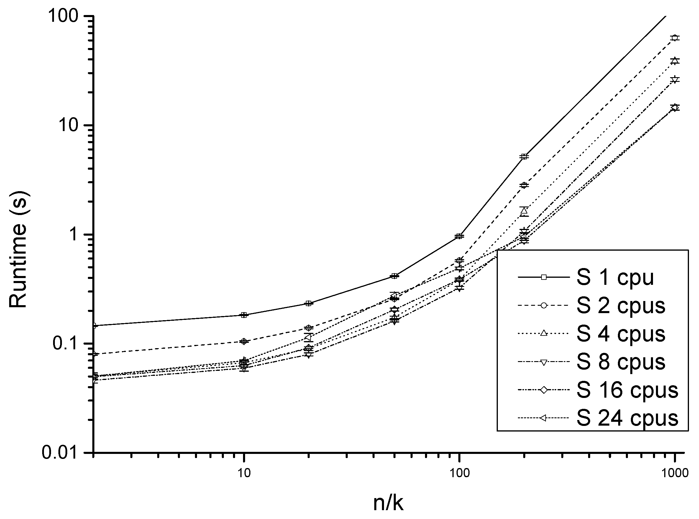
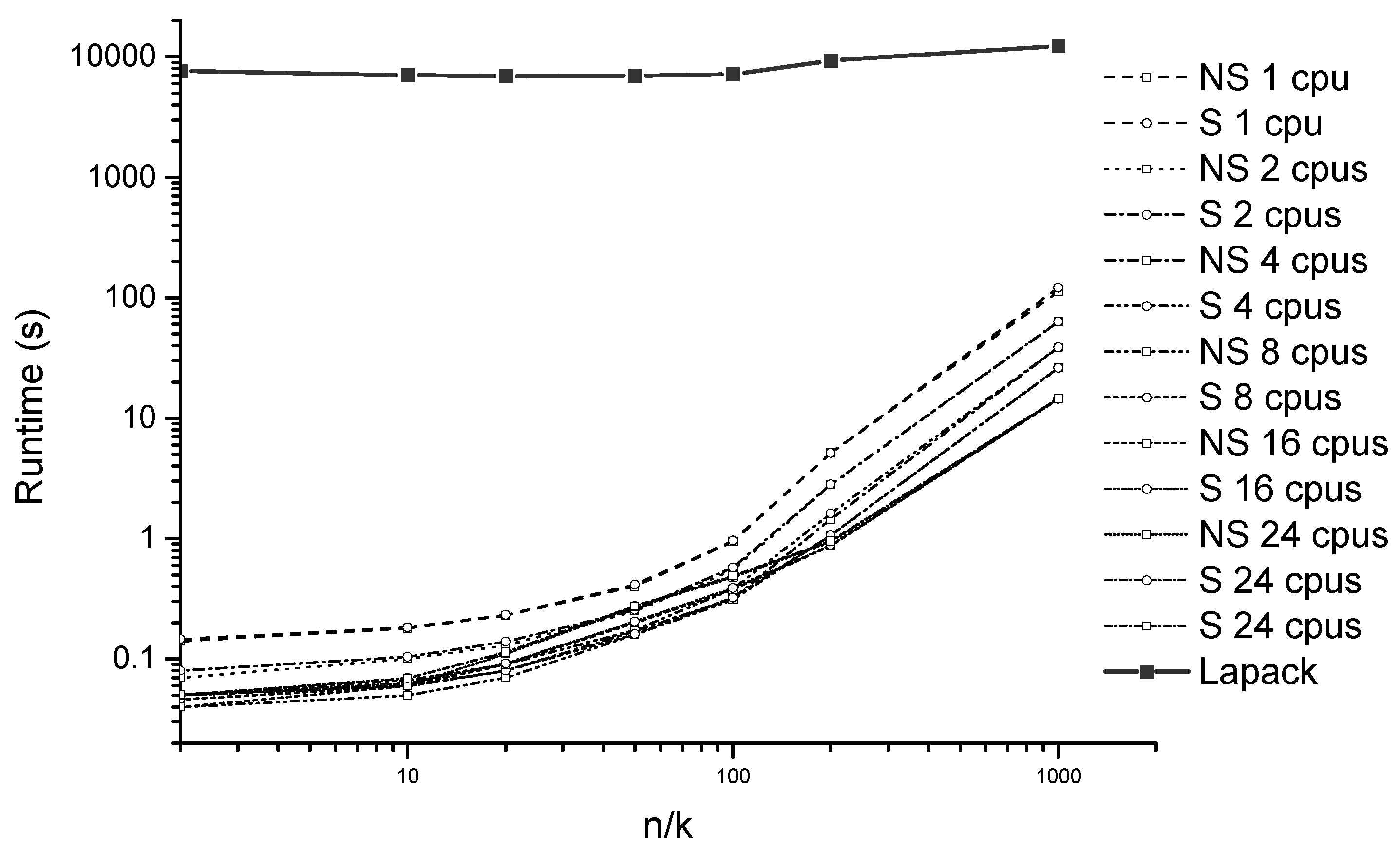
In this section, we exemplify our algorithm on a matrix similar to those considered by other authors [22,30], and another that also highlights the fact that our algorithm also handles non-symmetric matrices.

Firstly, we consider the matrix

$$\mathbf{T}=\left[\begin{array}{cccccccccc}1& 0& 0& 0& 1& 0& 0& 0& 0& 0\\ 0& 2& 0& 0& 0& 1& 0& 0& 0& 0\\ 0& 0& 2& 0& 0& 0& 1& 0& 0& 0\\ 0& 0& 0& 2& 0& 0& 0& 1& 0& 0\\ 1& 0& 0& 0& 2& 0& 0& 0& 1& 0\\ 0& 1& 0& 0& 0& 2& 0& 0& 0& 1\\ 0& 0& 1& 0& 0& 0& 2& 0& 0& 0\\ 0& 0& 0& 1& 0& 0& 0& 2& 0& 0\\ 0& 0& 0& 0& 1& 0& 0& 0& 2& 0\\ 0& 0& 0& 0& 0& 1& 0& 0& 0& 2\end{array}\right],$$

or, equivalently,

$$\mathbf{d}=\left[1,2,2,2,2,2,2,2,2,2\right];\mathbf{a}=\mathbf{b}=\left[1,1,1,1,1,1\right]$$

We then obtain the block-diagonal form of $\mathbf{T}$,

$${\mathbf{T}}^1=\left[\begin{array}{ccc}1& 1& 0\\ 1& 2& 1\\ 0& 1& 2\end{array}\right];{\mathbf{T}}^2=\left[\begin{array}{ccc}2& 1& 0\\ 1& 2& 1\\ 0& 1& 2\end{array}\right];{\mathbf{T}}^3={\mathbf{T}}^4=\left[\begin{array}{cc}2& 1\\ 1& 2\end{array}\right].$$

Now, we perform the SVD on each block, as follows

$${\mathbf{T}}^1\approx \left[\begin{array}{ccc}-0.328& 0.591& 0.737\\ -0.737& 0.328& -0.591\\ -0.591& -0.737& 0.328\end{array}\right]\left[\begin{array}{ccc}3.247& 0& 0\\ 0& 1.555& 0\\ 0& 0& 0.198\end{array}\right]{\left[\begin{array}{ccc}-0.328& 0.591& 0.737\\ -0.737& 0.328& -0.591\\ -0.591& -0.737& 0.328\end{array}\right]}^{\mathsf{T}},$$

$${\mathbf{T}}^2\approx \left[\begin{array}{ccc}-0.500& 0.707& 0.500\\ -0.707& -0.000& -0.707\\ -0.500& -0.707& 0.500\end{array}\right]\left[\begin{array}{ccc}3.414& 0& 0\\ 0& 2.000& 0\\ 0& 0& 0.586\end{array}\right]{\left[\begin{array}{ccc}-0.500& 0.707& 0.500\\ -0.707& -0.000& -0.707\\ -0.500& -0.707& 0.500\end{array}\right]}^{\mathsf{T}},$$

$${\mathbf{T}}^3={\mathbf{T}}^4\approx \left[\begin{array}{cc}-0.707& -0.707\\ -0.707& 0.707\end{array}\right]\left[\begin{array}{cc}3.000& 0\\ 0& 1.000\end{array}\right]{\left[\begin{array}{cc}-0.707& -0.707\\ -0.707& 0.707\end{array}\right]}^{\mathsf{T}}.$$

The augmented vectors ${\mathbf{v}}^i$ are

$$\begin{array}{cc}\hfill {\mathbf{v}}^1\approx & {\left[\begin{array}{ccc}-3.247& -1.555& -0.198\\ 1& 1& 1\\ 1& 2& 3\end{array}\right]}^{\mathsf{T}},\hfill \\ \hfill {\mathbf{v}}^2\approx & {\left[\begin{array}{ccc}-3.414& -2.000& -0.586\\ 2& 2& 2\\ 1& 2& 3\end{array}\right]}^{\mathsf{T}},\hfill \\ \hfill {\mathbf{v}}^3\approx & {\left[\begin{array}{cc}-3.000& -1.000\\ 3& 3\\ 1& 2\end{array}\right]}^{\mathsf{T}},{\mathbf{v}}^4\approx {\left[\begin{array}{cc}-3.000& -1.000\\ 4& 4\\ 1& 2\end{array}\right]}^{\mathsf{T}},\hfill \end{array}$$

and thus the merged vector $\mathbf{v}$ is

$$\mathbf{v}\approx {\left[\begin{array}{cccccccccc}-3.414& -3.247& -3.000& -3.000& -2.000& -1.555& -1.000& -1.000& -0.586& -0.198\\ 2& 1& 3& 4& 2& 1& 3& 4& 2& 1\\ 1& 1& 1& 1& 2& 2& 2& 2& 3& 3\end{array}\right]}^{\mathsf{T}}$$

from which, we obtain the column selectors ${\mathbf{c}}^i$,

$${\mathbf{c}}^1={\left[\begin{array}{ccc}2& 6& 10\end{array}\right]}^{\mathsf{T}}{\mathbf{c}}^2={\left[\begin{array}{ccc}1& 5& 9\end{array}\right]}^{\mathsf{T}}{\mathbf{c}}^3={\left[\begin{array}{cc}3& 7\end{array}\right]}^{\mathsf{T}}{\mathbf{c}}^4={\left[\begin{array}{cc}4& 8\end{array}\right]}^{\mathsf{T}}$$

while the original row selectors ${\mathbf{s}}^i$ were,

$${\mathbf{s}}^1={\left[\begin{array}{ccc}1& 5& 9\end{array}\right]}^{\mathsf{T}}{\mathbf{s}}^2={\left[\begin{array}{ccc}2& 6& 10\end{array}\right]}^{\mathsf{T}}{\mathbf{s}}^3={\left[\begin{array}{cc}3& 7\end{array}\right]}^{\mathsf{T}}{\mathbf{s}}^4={\left[\begin{array}{cc}4& 8\end{array}\right]}^{\mathsf{T}}$$

hence, we obtain the decomposition

$$\mathbf{U}=\mathbf{V}=\left[\begin{array}{cccccccccc}0& -0.328& 0& 0& 0& 0.591& 0& 0& 0& -0.737\\ -0.500& -0& 0& 0& -0.707& 0& 0& 0& 0.500& 0\\ 0& 0& -0.707& 0& 0& 0& -0.707& 0& 0& 0\\ 0& 0& 0& -0.707& 0& 0& 0& -0.707& 0& 0\\ 0& -0.737& 0& 0& 0& 0.328& 0& 0& 0& 0.591\\ -0.707& 0& 0& 0& 0& 0& 0& 0& -0.707& 0\\ 0& 0& -0.707& 0& 0& 0& 0.707& 0& 0& 0\\ 0& 0& 0& -0.707& 0& 0& 0& 0.707& 0& 0\\ 0& -0.591& 0& 0& 0& -0.737& 0& 0& 0& -0.328\\ -0.500& 0& 0& 0& 0.707& 0& 0& 0& 0.500& 0\end{array}\right],$$

$$\mathbf{S}=\mathrm{diag}\left(\left[\begin{array}{cccccccccc}-3.414& -3.247& -3.000& -3.000& -2.000& -1.555& -1.000& -1.000& -0.586& -0.198\end{array}\right]\right).$$

Furthermore, we consider the matrix

$$\mathbf{T}=\left[\begin{array}{cccccccccc}1& 0& 0& 0& 1& 0& 0& 0& 0& 0\\ 0& 2& 0& 0& 0& 1& 0& 0& 0& 0\\ 0& 0& 2& 0& 0& 0& 1& 0& 0& 0\\ 0& 0& 0& 2& 0& 0& 0& 1& 0& 0\\ -1& 0& 0& 0& 2& 0& 0& 0& 1& 0\\ 0& -1& 0& 0& 0& 2& 0& 0& 0& 1\\ 0& 0& -1& 0& 0& 0& 2& 0& 0& 0\\ 0& 0& 0& -1& 0& 0& 0& 2& 0& 0\\ 0& 0& 0& 0& -1& 0& 0& 0& 2& 0\\ 0& 0& 0& 0& 0& -1& 0& 0& 0& 2\end{array}\right],$$

or, equivalently,

$$\mathbf{d}=\left[1,2,2,2,2,2,2,2,2,2\right];\mathbf{b}=-\mathbf{a}=-\left[1,1,1,1,1,1\right]$$

We then obtain the block-diagonal form of $\mathbf{T}$,

$${\mathbf{T}}^1=\left[\begin{array}{ccc}1& 1& 0\\ -1& 2& 1\\ 0& -1& 2\end{array}\right];{\mathbf{T}}^2=\left[\begin{array}{ccc}2& 1& 0\\ -1& 2& 1\\ 0& -1& 2\end{array}\right];{\mathbf{T}}^3={\mathbf{T}}^4=\left[\begin{array}{cc}2& 1\\ -1& 2\end{array}\right].$$

Now, we perform the SVD on each block, as follows

$${\mathbf{T}}^1\approx \left[\begin{array}{ccc}-0.268& -0.208& -0.940\\ -0.940& 0.268& 0.208\\ 0.208& 0.940& 0.268\end{array}\right]\left[\begin{array}{ccc}2.507& 0& 0\\ 0& 2.285& 0\\ 0& 0& 1.221\end{array}\right]{\left[\begin{array}{ccc}0.268& -0.208& -0.940\\ -0.940& -0.268& -0.208\\ -0.208& 0.940& -0.268\end{array}\right]}^{\mathsf{T}},$$

$${\mathbf{T}}^2\approx \left[\begin{array}{ccc}-0.408& -0.577& -0.707\\ -0.816& 0.577& 0.000\\ 0.408& 0.577& 0.500\end{array}\right]\left[\begin{array}{ccc}2.449& 0& 0\\ 0& 2.449& 0\\ 0& 0& 2.000\end{array}\right]{\left[\begin{array}{ccc}0.000& -0.707& -0.707\\ -1.000& 0.000& 0.000\\ 0.000& 0.707& -0.707\end{array}\right]}^{\mathsf{T}},$$

$${\mathbf{T}}^3={\mathbf{T}}^4\approx \left[\begin{array}{cc}-0.894& -0.447\\ -0.447& 0.894\end{array}\right]\left[\begin{array}{cc}2.236& 0\\ 0& 2.236\end{array}\right]{\left[\begin{array}{cc}-1& 0\\ -0& 1\end{array}\right]}^{\mathsf{T}}.$$

The augmented vectors ${\mathbf{v}}^i$ are

$$\begin{array}{cc}\hfill {\mathbf{v}}^1\approx & {\left[\begin{array}{ccc}-2.507& -2.285& -1.221\\ 1& 1& 1\\ 1& 2& 3\end{array}\right]}^{\mathsf{T}},\hfill \\ \hfill {\mathbf{v}}^2\approx & {\left[\begin{array}{ccc}-2.449& -2.449& -2.000\\ 2& 2& 2\\ 1& 2& 3\end{array}\right]}^{\mathsf{T}},\hfill \\ \hfill {\mathbf{v}}^3\approx & {\left[\begin{array}{cc}-2.236& -2.236\\ 3& 3\\ 1& 2\end{array}\right]}^{\mathsf{T}},{\mathbf{v}}^4\approx {\left[\begin{array}{cc}-2.236& -2.236\\ 4& 4\\ 1& 2\end{array}\right]}^{\mathsf{T}},\hfill \end{array}$$

and thus, the merged vector $\mathbf{v}$ is

$$\mathbf{v}\approx {\left[\begin{array}{cccccccccc}-2.507& -2.449& -2.449& -2.285& -2.236& -2.236& -2.236& -2.236& -2.000& -1.221\\ 1& 2& 2& 1& 3& 3& 4& 4& 2& 1\\ 1& 1& 2& 2& 1& 2& 1& 2& 3& 3\end{array}\right]}^{\mathsf{T}}$$

from which, we obtain the column selectors ${\mathbf{c}}^i$,

$${\mathbf{c}}^1={\left[\begin{array}{ccc}1& 4& 10\end{array}\right]}^{\mathsf{T}}{\mathbf{c}}^2={\left[\begin{array}{ccc}2& 3& 9\end{array}\right]}^{\mathsf{T}}{\mathbf{c}}^3={\left[\begin{array}{cc}5& 6\end{array}\right]}^{\mathsf{T}}{\mathbf{c}}^4={\left[\begin{array}{cc}7& 8\end{array}\right]}^{\mathsf{T}}$$

while the original row selectors ${\mathbf{s}}^i$ were

$${\mathbf{s}}^1={\left[\begin{array}{ccc}1& 5& 9\end{array}\right]}^{\mathsf{T}}{\mathbf{s}}^2={\left[\begin{array}{ccc}2& 6& 10\end{array}\right]}^{\mathsf{T}}{\mathbf{s}}^3={\left[\begin{array}{cc}3& 7\end{array}\right]}^{\mathsf{T}}{\mathbf{s}}^4={\left[\begin{array}{cc}4& 8\end{array}\right]}^{\mathsf{T}}$$

hence, we obtain the decomposition

$$\mathbf{U}=\left[\begin{array}{cccccccccc}-0.268& 0& 0& -0.208& 0& 0& 0& 0& 0& -0.940\\ 0& -0.408& -0.577& 0& 0& 0& 0& 0& -0.707& 0\\ 0& 0& 0& 0& -0.894& 0.447& 0& 0& 0& 0\\ 0& 0& 0& 0& 0& 0& -0.894& 0.447& 0& 0\\ -0.940& 0& 0& 0.268& 0& 0& 0& 0& 0& 0.208\\ 0& -0.816& 0.577& 0& 0& 0& 0& 0& 0.000& 0\\ 0& 0& 0& 0& 0.447& 0.894& 0& 0& 0& 0\\ 0& 0& 0& 0& 0& 0& -0.894& 0.447& 0& 0\\ 0.208& 0& 0& 0.940& 0& 0& 0& 0& 0& -0.268\\ 0& 0.408& 0.577& 0& 0& 0& 0& 0& -0.707& 0\end{array}\right],$$

$$-\mathbf{S}=\mathrm{diag}\left(\left[\begin{array}{cccccccccc}-2.507& -2.449& -2.449& -2.285& -2.236& -2.236& -2.236& -2.236& -2.000& -1.221\end{array}\right]\right).$$

$$\mathbf{V}=\left[\begin{array}{cccccccccc}0.268& 0& 0& -0.208& 0& 0& 0& 0& 0& -0.940\\ 0& 0.000& -0.707& 0& 0& 0& 0& 0& -0.707& 0\\ 0& 0& 0& 0& -1.000& 0.000& 0& 0& 0& 0\\ 0& 0& 0& 0& 0& 0& -1.000& 0.000& 0& 0\\ -0.940& 0& 0& -0.268& 0& 0& 0& 0& 0& -0.208\\ 0& -1.000& 0.000& 0& 0& 0& 0& 0& 0.000& 0\\ 0& 0& 0& 0& 0.000& 1.000& 0& 0& 0& 0\\ 0& 0& 0& 0& 0& 0& 0.000& 1.000& 0& 0\\ -0.208& 0& 0& 0.940& 0& 0& 0& 0& 0& -0.268\\ 0& 0.000& 0.707& 0& 0& 0& 0& 0& -0.707& 0\end{array}\right],$$

5. Evaluation

In this section, we present a comparison between Algorithm 1 and the industry standard for full SVD implementations, the Lapack library. We used Lapack DGESVD rutine, the standard method. It computes the SVD of a real $n\times m$ matrix, optionally computing the left and/or right singular vectors. Our code was developed to obtain real results on many random matrix inputs, and to show that Lapack does indeed not know to take advantage of $n/k$. Experimental data serves to validate Theorem 1, and, given the small RSD, it can clearly be extrapolated.

Regarding the dataset, any bidiagonal or tridiagonal matrix dataset can be used, using any black box solver, like the one presented in [31]. However, such matrices are only 1-tridiagonal; thus, our algorithm will simply be called the black box. To our knowledge, there is no standard k-tridiagonal matrix dataset, which is why we generated random matrices.

In order to validate and compare our scalability of k-tridiagonal matrix singular value decomposition, we have built an experimental infrastructure using dedicated computing servers. The compute node used is a dual-socket one with a CPU architecture based on XEON E5-2640 v3 running at 2.60 GHz. It has 16 cores and 32 hyper-threads (hyper-threading enabled). The amount of memory available is 128 GB RAM, which is relevant for the size of the matrix you can load in the memory. Being a shared cluster, we have used a shared NFS storage connected through 10Gbps ethernet. The NFS backend is formed of 900 GB SAS disks in RAID6 (this is relevant for the time needed to read the input matrix). The amount of memory and storage description was given here for practical purposes, but was not taken into account in our measurements and comparisons. In our experimental setup, we measured the amount of time needed for computing the k-tridiagonal matrix singular value decomposition (without reading and writing the inputs and outputs). Regarding the software base, the compute node was running a CentOS7, with the latest updates of the time of writing this paper (CentOS 7.7), and a hand built compiler gcc gnu-5.4.0 (to take full advantage of the architecture). The parallelization was performed using OpenMP flags (so multi-threaded).

Please note that the 24-core experiment uses the hyper-threads, which are not as efficient as a fully-fledged core, but we wanted to see how it scales.

We firstly investigate the reliability of our measurements. We evaluate our method on 10,000 × 10,000 k-tridiagonal matrices with entries of uniformly distributed integers in the interval $\left[0, 100\right]$ for various values of k (10, 50, 100, 200, 500, 1000, 5000) using multiple setups (1, 2, 4, 8, 16, 24 CPUs). We perform 1000 such experiments and plot the mean and standard deviation of our proposed code in Figure 1. The variability of this method can be quantified by the relative standard deviation (RSD), which varies between 1.05% and 9.95% for the measurements we have performed.

Finally, we evaluate whether industry standard software, such as Lapack, can detect and use the sparsity of our data. We consider $10,000\times 10,0000$ matrices with entries of uniformly distributed integers in the interval $\left[0, 100\right]$, and multiple values of k (10, 50, 100, 200, 500, 1000, 5000). We plot in Figure 2 the mean runtime of Lapack, the parallel code of [30] and our proposed code, where the parallel codes are ran on 1, 2, 4, 8, 16, 24 cpus. From the graph, we can see that sorting the eigenvalues adds almost no cost (<5 ms), and that both methods produce much better results than Lapack. Thus, considering its low variability, our method provides a great improvement over Lapack, not only on average, but even in the worst cases.

While many algorithms have been developed for general banded matrices, the k-tridiagonal form allows for even further optimization. For example, notice that, as the matrix becomes wider-banded (i.e., as k increases), our algorithm gets better whereas the previous algorithm [32] gets worse, i.e., when $k=n$, the previous algorithm is worse than the traditional full-matrix BCD SVD.

6. Conclusions

Considering the great theoretical improvement of singular value decomposition for k-tridiagonal matrices [30] as a starting point, we proved here that sorting the singular values does not alter the performance, nor the scaling potential. Furthermore, a complete scaling scenario has been treated, showing surprising results, which emphasize the endless scalability potential of such methods, providing a considerable burst to industry standard implementations. The singular value decomposition method is a very important tool that is core to the development of new technologies especially in communications, so any new improved implementation adds a valuable benefit.

References

1. Horn, R.A.; Horn, R.A.; Johnson, C.R. Matrix Analysis; Cambridge University Press: Cambridge, UK, 1990. [Google Scholar]
2. Bishop, C.M. Pattern Recognition and Machine Learning; Springer Science+ Business Media: New York, NY, USA, 2006. [Google Scholar]
3. Jolliffe, I.T.; Cadima, J. Principal component analysis: A review and recent developments. Philos. Trans. R. Soc. A Math. Phys. Eng. Sci. 2016, 374, 20150202. [Google Scholar] [CrossRef] [PubMed]
4. Luo, W.H.; Huang, T.Z.; Gu, X.M.; Liu, Y. Barycentric rational collocation methods for a class of nonlinear parabolic partial differential equations. Appl. Math. Lett. 2017, 68, 13–19. [Google Scholar] [CrossRef]
5. McMillen, T.; Bourget, A.; Agnew, A. On the zeros of complex Van Vleck polynomials. J. Comput. Appl. Math. 2009, 223, 862–871. [Google Scholar] [CrossRef] [Green Version]
6. Gu, X.M.; Sun, H.W.; Zhao, Y.L.; Zheng, X. An implicit difference scheme for time-fractional diffusion equations with a time-invariant type variable order. Appl. Math. Lett. 2021, 120, 107270. [Google Scholar] [CrossRef]
7. Luo, W.H.; Gu, X.M.; Yang, L.; Meng, J. A Lagrange-quadratic spline optimal collocation method for the time tempered fractional diffusion equation. Math. Comput. Simul. 2021, 182, 1–24. [Google Scholar] [CrossRef]
8. Peng, W.; Xin, B. An integrated autoencoder-based filter for sparse big data. J. Control. Decis. 2020, 8, 260–268. [Google Scholar] [CrossRef]
9. Ruble, M.; Güvenç, İ. Multilinear Singular Value Decomposition for Millimeter Wave Channel Parameter Estimation. IEEE Access 2020, 8, 75592–75606. [Google Scholar] [CrossRef]
10. He, Y.L.; Tian, Y.; Xu, Y.; Zhu, Q.X. Novel soft sensor development using echo state network integrated with singular value decomposition: Application to complex chemical processes. Chemom. Intell. Lab. Syst. 2020, 200, 103981. [Google Scholar] [CrossRef]
11. Han, S.; Ng, W.K.; Philip, S.Y. Privacy-preserving singular value decomposition. In Proceedings of the 2009 IEEE 25th International Conference on Data Engineering, Shanghai, China, 29 March–2 April 2009; pp. 1267–1270. [Google Scholar]
12. Chan, T.F. An improved algorithm for computing the singular value decomposition. ACM Trans. Math. Softw. (TOMS) 1982, 8, 72–83. [Google Scholar] [CrossRef]
13. Gu, M.; Eisenstat, S.C. A divide-and-conquer algorithm for the bidiagonal SVD. SIAM J. Matrix Anal. Appl. 1995, 16, 79–92. [Google Scholar] [CrossRef]
14. Nakatsukasa, Y.; Higham, N.J. Stable and efficient spectral divide and conquer algorithms for the symmetric eigenvalue decomposition and the SVD. SIAM J. Sci. Comput. 2013, 35, A1325–A1349. [Google Scholar] [CrossRef]
15. de Rijk, P. A one-sided Jacobi algorithm for computing the singular value decomposition on a vector computer. SIAM J. Sci. Stat. Comput. 1989, 10, 359–371. [Google Scholar] [CrossRef]
16. Konda, T.; Nakamura, Y. A new algorithm for singular value decomposition and its parallelization. Parallel Comput. 2009, 35, 331–344. [Google Scholar] [CrossRef]
17. Musco, C.; Musco, C. Randomized block Krylov methods for stronger and faster approximate singular value decomposition. In Proceedings of the Annual Conference on Neural Information Processing Systems 2015, Montreal, QC, Canada, 7–12 December 2015; pp. 1396–1404. [Google Scholar]
18. Kokiopoulou, E.; Bekas, C.; Gallopoulos, E. Computing smallest singular triplets with implicitly restarted Lanczos bidiagonalization. Appl. Numer. Math. 2004, 49, 39–61. [Google Scholar] [CrossRef] [Green Version]
19. Niu, D.; Yuan, X. An implicitly restarted Lanczos bidiagonalization method with refined harmonic shifts for computing smallest singular triplets. J. Comput. Appl. Math. 2014, 260, 208–217. [Google Scholar] [CrossRef]
20. Ishida, Y.; Takata, M.; Kimura, K.; Nakamura, Y. An Improvement of Augmented Implicitly Restarted Lanczos Bidiagonalization Method. In Proceedings of the International Conference on Parallel and Distributed Processing Techniques and Applications (PDPTA). The Steering Committee of The World Congress in Computer Science, Computer Engineering and Applied Computing (WorldComp), Las Vegas, NV, USA, 17–20 July 2017; pp. 281–287. [Google Scholar]
21. Sogabe, T.; El-Mikkawy, M. Fast block diagonalization of k-tridiagonal matrices. Appl. Math. Comput. 2011, 218, 2740–2743. [Google Scholar] [CrossRef]
22. El-Mikkawy, M.; Atlan, F. A novel algorithm for inverting a general k-tridiagonal matrix. Appl. Math. Lett. 2014, 32, 41–47. [Google Scholar] [CrossRef]
23. El-Mikkawy, M.; Atlan, F. A new recursive algorithm for inverting general k-tridiagonal matrices. Appl. Math. Lett. 2015, 44, 34–39. [Google Scholar] [CrossRef]
24. Sogabe, T.; Yılmaz, F. A note on a fast breakdown-free algorithm for computing the determinants and the permanents of k-tridiagonal matrices. Appl. Math. Comput. 2014, 249, 98–102. [Google Scholar] [CrossRef]
25. Kirklar, E.; Yilmaz, F. A Note on k-Tridiagonal k-Toeplitz Matrices. Ala. J. Math. 2015, 3, 39. [Google Scholar]
26. Jia, J.; Li, S. Symbolic algorithms for the inverses of general k-tridiagonal matrices. Comput. Math. Appl. 2015, 70, 3032–3042. [Google Scholar] [CrossRef]
27. Ohashi, A.; Usuda, T.; Sogabe, T. On Tensor product decomposition of k-tridiagonal toeplitz matrices. Int. J. Pure Appl. Math. 2015, 103, 537–545. [Google Scholar] [CrossRef]
28. Takahira, S.; Sogabe, T.; Usuda, T. Bidiagonalization of (k, k+ 1)-tridiagonal matrices. Spec. Matrices 2019, 7, 20–26. [Google Scholar] [CrossRef]
29. Küçük, A.Z.; Özen, M.; İnce, H. Recursive and Combinational Formulas for Permanents of General k-tridiagonal Toeplitz Matrices. Filomat 2019, 33, 307–317. [Google Scholar]
30. Tănăsescu, A.; Popescu, P.G. A fast singular value decomposition algorithm of general k-tridiagonal matrices. J. Comput. Sci. 2019, 31, 1–5. [Google Scholar] [CrossRef]
31. Marques, O.; Demmel, J.; Vasconcelos, P.B. Bidiagonal SVD Computation via an Associated Tridiagonal Eigenproblem. ACM Trans. Math. Softw. (TOMS) 2020, 46, 1–25. [Google Scholar] [CrossRef]
32. Liao, X.; Li, S.; Cheng, L.; Gu, M. An improved divide-and-conquer algorithm for the banded matrices with narrow bandwidths. Comput. Math. Appl. 2016, 71, 1933–1943. [Google Scholar] [CrossRef]
Figure 1. Average runtime of our proposed algorithm for n = 10,000 and multiple values of k and multiple numbers of cpus.
Mathematics 09 03123 g001
Figure 2. Average runtime of our proposed algorithm (marked S in the legend), the algorithm of [30] (marked NS in the legend) and Lapack for n = 10 , 000 and multiple values of k and multiple numbers of cpus.
Mathematics 09 03123 g002
Publisher’s Note: MDPI stays neutral with regard to jurisdictional claims in published maps and institutional affiliations.