An Extended log-Lindley-G Family: Properties and Experiments in Repairable Data

Abstract

In this article, two new families of distributions are proposed: the generalized log-Lindley-G (GLL-G) and its counterpart, the GLL*-G. These families can be justified by their relation to the log-Lindley model, an important assumption for describing social and economic phenomena. Specific GLL models are introduced and studied. We show that the GLL density is rewritten as a two-member linear combination of the exponentiated G-densities and that, consequently, many of its mathematical properties arise directly, such as moment-based expressions. A maximum likelihood estimation procedure for the GLL parameters is provided and the behavior of the resulting estimates is evaluated by Monte Carlo experiments. An application to repairable data is made. The results argue for the use of the exponential law as the basis for the GLL-G family.

1. Introduction

Providing flexible and accurate distributions is sought in a variety of contexts, including public health, biomedical studies, and reliability (for a fuller discussion, see [1]). Lindley [2] pioneered the one-parameter Lindley distribution, to which several extensions have been developed [3]. Abouammoh and Kayid [4] developed a general form for Lindey-based extended models. Al-Babtain et al. [5] proposed a new version for a discrete analog of the continuous Lindley law. Beyond extensions of the Lindley distribution, improved statistical inference tools have been derived from it [6,7,8,9].

Recently, Gómez-Déniz et al. [10] have proposed the log-Lindley (LL) distribution with probability density function (pdf)

$$f(x;\lambda ,\sigma )=\frac{{\sigma }^2}{1+\lambda \sigma }(\lambda -logx)x^{\sigma -1},0<x<1,\lambda \ge 0,\sigma >0.$$

(1)

According to Zakerzadeh and Dolati [11], this distribution may be also developed from the generalized Lindley law and has simple moment-based expressions and important reliability properties. The new model has been successfully applied in the current context on which the LL cdf is often used to misinterpret the prime principle (Gómez-Déniz et al. [10]). Our proposal is an alternative to the family proposed by Jones [12], who furnished a flexible family of models from Beta random variables. This family of distributions is able to model symmetric and skewed data sets with varying tail weights. Further, Zografos and Balakrishnan [13], Ristic and Balakrishnan [14] and Amini et al. [15] suggested a family of distributions spawned from the gamma random variables. In a similar vein, we present two new families of distributions generated from log-Lindley random variables through the following definition.

Recently, Alzaatreh et al. [16] introduced the T-X family—constructed from a random variable $T\in [a,b]$ for $a<b$ with density $r\left(t\right)$—having cumulative distribution function (cdf)

$$F\left(x\right)={\int }_a^{L\left[G\right(x\left)\right]}r\left(t\right)\mathrm{d}t,$$

(2)

and its associated pdf is

$$f\left(x\right)=\left\{\frac{d}{dx}L\left[G\left(x\right)\right]\right\}r\left(L\left[G\right(x\left)\right]\right),$$

(3)

where $L\left[G\right(x\left)\right]$ satisfies the following conditions: i. $L\left[G\right(x\left)\right]\in [a,b]$; ii. $L\left[G\right(x\left)\right]$ is differentiable and non-descending monotonous; and iii. $L\left[G\right(x\left)\right]\to a$ when $x\to -\infty$ and $L\left[G\right(x\left)\right]\to b$ when $x\to \infty$.

Based on the T-X generator defined by Equation (2), we introduce two new families of continuous distributions termed generalized log-Lindley-G distributions by integrating the LL density function.

Definition 1.

Denote $F(·)$ and $\overline{F}(·)$ as the cdf and the survival function of a random variable with the pdf $f(·)$. We announce two new families of distributions having pdfs

$$g_{\overline{F}}(x;\lambda ,\sigma )=\frac{{\sigma }^2}{1+\lambda \sigma }\left(\lambda -log\overline{F}\left(x\right)\right)\overline{F}{\left(x\right)}^{\sigma -1}f\left(x\right)$$

(4)

and

$$g_F(x;\lambda ,\sigma )=\frac{{\sigma }^2}{1+\lambda \sigma }\left(\lambda -logF\left(x\right)\right)F{\left(x\right)}^{\sigma -1}f\left(x\right).$$

(5)

The proposed family can actually be obtained from the log-Lindley family of Gómez-Déniz et al. [10] and the T-X generator, taking into account the integrals

$${\overline{G}}_{\overline{F}}(x;\lambda ,\sigma )=\frac{{\sigma }^2}{1+\lambda \sigma }{\int }_0^{\overline{F}\left(x\right)}(\lambda -logt)t^{\sigma -1}\mathrm{d}t$$

(6)

and

$$G_F(x;\lambda ,\sigma )=\frac{{\sigma }^2}{1+\lambda \sigma }{\int }_0^{F\left(x\right)}(\lambda -logt)t^{\sigma -1}\mathrm{d}t,$$

(7)

respectively.

First, we define the density functions of $r\left(t\right)$ in (2) as

$$r_{\overline{F}}(t;\lambda ,\sigma )=\frac{{\sigma }^2}{1+\lambda \sigma }\left[\lambda -log(1-t)\right]{(1-t)}^{\sigma -1},0<t<1,$$

(8)

and

$$r_F(t;\lambda ,\sigma )=\frac{{\sigma }^2}{1+\lambda \sigma }\left[\lambda -log\left(t\right)\right]t^{\sigma -1},0<t<1,$$

(9)

and replacing $L\left[G\right(x\left)\right]$ by $G^{\alpha }\left(x\right)$ in (2), we have the two cdf of the generalized log-Lindley-G family, respectively, as

$$\begin{array}{cc}\hfill F^{*}(x;\alpha ,\lambda ,\sigma ,\mathbf{\zeta })& =\frac{{\sigma }^2}{1+\lambda \sigma }{\int }_0^{G^{\alpha }(x;\mathbf{\zeta })}\left(\lambda -log[1-t]\right){(1-t)}^{\sigma -1}\mathrm{d}t\hfill \\ \hfill & =1-\frac{1}{1+\lambda \sigma }{\left[1-G^{\alpha }(x;\mathbf{\zeta })\right]}^{\sigma }\left\{1+\sigma [\lambda -log(1-G^{\alpha }(x;\mathbf{\zeta }))]\right\}\hfill \end{array}$$

(10)

and

$$\begin{array}{cc}\hfill F(x;\alpha ,\lambda ,\sigma ,\mathbf{\zeta })& =\frac{{\sigma }^2}{1+\lambda \sigma }{\int }_0^{G^{\alpha }(x;\mathbf{\zeta })}\left(\lambda -log\left[t\right]\right)t^{\sigma -1}\mathrm{d}t\hfill \\ \hfill & =\frac{1}{1+\lambda \sigma }{G}^{\alpha \sigma }(x;\mathbf{\zeta })\left\{1+\sigma [\lambda -log\left(G^{\alpha }(x;\mathbf{\zeta })\right)]\right\},\hfill \end{array}$$

(11)

where $G(x;\mathbf{\zeta })$ and $g(x;\mathbf{\zeta })$ depend on a parameter vector $\mathbf{\zeta }$ and $\alpha ,\lambda ,\sigma$ are three additional parameters. Henceforth, we will refer to these families as GLL-G, $F(·)$, and ${\mathrm{GLL}}^{*}$-G, $F^{*}(·)$ families.

The structure of the paper is as follows. In Section 2 we propose two new families of distributions arising from the LL model. Section 3 brings some special models in these families. In Section 4 we derive an extension for the density of the family GLL-G. In Section 5, we derive several mathematical properties of the GLL-G family, including, along with ordinary and incomplete moments, mean deviations and the moments of residual and reversed lifetime. Rényi, Shannon, and Mathai-Haubold entropies and order statistics are studied in Section 6 and  Section 7, respectively. An estimation procedure for the GLL-G parameters is given in Section 8. Section 9 and Section 10 deal with the numerical results, while Section 11 contains the concluding thoughts.

2. The GLL-G Family

Here, we introduce two new families of distributions having cdfs (10) and (11) by incorporating two additional shape parameters, $\alpha >0$ and $\sigma >0$, and one scale parameter, $\lambda \ge 0$, to yield a more flexible generator. By differentiating (10) and (11), the associated pdfs are, respectively,

$$\begin{array}{cc}\hfill f^{*}(x;\alpha ,\lambda ,\sigma ,\mathbf{\zeta })=& \frac{\alpha {\sigma }^2}{1+\lambda \sigma }g(x;\zeta )G^{\alpha -1}(x;\mathbf{\zeta }){\left(1-G^{\alpha }(x;\mathbf{\zeta })\right)}^{\sigma -1}\hfill \\ \hfill & \times \left(\lambda -log[1-G^{\alpha }(x;\mathbf{\zeta })]\right)\hfill \end{array}$$

(12)

and

$$f(x;\alpha ,\lambda ,\sigma ,\zeta )=\frac{\alpha {\sigma }^2}{1+\lambda \sigma }g(x;\zeta )G^{\alpha \sigma -1}(x;\mathbf{\zeta })\left(\lambda -log\left[G^{\alpha }(x;\mathbf{\zeta })\right]\right).$$

(13)

The hazard rate functions (hrfs) of the proposed families defined in (10) and (11) are given as

$$h^{*}(x;\alpha ,\lambda ,\sigma ,\mathbf{\zeta })=\frac{\alpha \sigma g(x;\mathbf{\zeta })G^{\alpha -1}(x;\mathbf{\zeta })\left(\lambda -log\left[1-G^{\alpha }(x;\mathbf{\zeta })\right]\right)}{(1-G^{\alpha }(x;\mathbf{\zeta }))\left[1+\sigma (\lambda -log[1-G^{\alpha }(x;\mathbf{\zeta })])\right]}$$

and

$$h(x;\alpha ,\lambda ,\sigma ,\zeta )=\frac{\alpha \sigma g(x;\mathbf{\zeta })\left(\lambda -log\left[G^{\alpha }(x;\mathbf{\zeta })\right]\right)}{G(x;\mathbf{\zeta })[\sigma log\left[G^{\alpha }(x;\mathbf{\zeta })\right]-(1+\lambda \sigma )(1-G^{-\alpha \sigma }(x;\mathbf{\zeta }))]},$$

(14)

respectively.

Now, we offer expressions for the quantile functions related to (10) and (11). Based on the work of Jodrá and Jiménez-Gamero [17], it holds from $F\left(X\right)=U$ and $F^{*}\left(X^{*}\right)=U$ that, respectively,

$$X=Q_{\mathrm{baseline}}\left({exp}^{1/\alpha \sigma }\left(1+\lambda \sigma \right){exp}^{1/\alpha \sigma }\left\{W\left[\frac{-U(1+\lambda \sigma )}{exp(1+\lambda \sigma )}\right]\right\}\right),$$

(15)

and

$$X^{*}=Q_{\mathrm{baseline}}\left({\left[1-{exp}^{1/\sigma }\left(1+\lambda \sigma \right){exp}^{1/\sigma }\left\{W\left[\frac{-(1-U)(1+\lambda \sigma )}{exp(1+\lambda \sigma )}\right]\right\}\right]}^{1/\alpha }\right),$$

(16)

where $W(·)$ is the secondary branch Lambert W function. The last identities furnish random number generators (RNGs) for distributions $F^{*}(·)$ and $F(·)$.

Some notable existing members of the families (12) and (13) are introduced in

Table 1. Particular and special cases defined from the proposed families. ${\mathbb{I}}_A\left(x\right)$ means the indicator function in set A.

Family	Survival Function (Parameter Restriction)	Density	Reference
Lindley distribution
$f^{*}\left(x\right)$	$1-G\left(x\right)=exp\{-\lambda x\}$ ($\alpha =1$ and $\eta =\sigma \lambda$)	$f^{*}\left(x\right)=\frac{{\eta }^2}{1+\eta }(1+x)exp\{-\eta x\}{\mathbb{I}}_{(0,\infty )}\left(x\right)$	[18]
log-Lindley distribution
$f\left(x\right)$	$G\left(x\right)=x$ ($\alpha =1$ and $\eta =\sigma \lambda$)	$f\left(x\right)=\frac{{\sigma }^2}{1+\lambda \sigma }(\lambda -logx)x^{\sigma -1}{\mathbb{I}}_{(0,1)}\left(x\right)$	[10]
Power-Lindley distribution
$f^{*}\left(x\right)$	$\overline{G}\left(x\right)=exp\left\{\lambda x^{\beta }\right\}$ ($\alpha =1$)	$f^{*}\left(x\right)=\frac{\beta {\eta }^2}{1+\eta }(1+x^{\beta })x^{\beta -1}exp\{-\eta x^{\beta }\}{\mathbb{I}}_{(0,\infty )}\left(x\right)$	[19]
Power log-Lindley distribution
$f\left(x\right)$	$\overline{G}\left(x\right)=x$	$f\left(x\right)=\frac{\alpha {\sigma }^2}{1+\lambda \sigma }(\lambda -log{x}^{\alpha })x^{\alpha \sigma -1}{\mathbb{I}}_{(0,1)}\left(x\right)$	[new]
The inverse-Lindley distribution
$f\left(x\right)$	$G\left(x\right)=exp\{-\lambda x^{-1}\}$ ($\alpha =1$)	$f\left(x\right)=\frac{{\eta }^2}{1+\eta }\left(\frac{1+x}{x^3}\right)exp\{-\eta x^{-1}\}{\mathbb{I}}_{(0,\infty )}\left(x\right)$	[20]
The inverse power Lindley distribution
$f\left(x\right)$	$G\left(x\right)=exp\{-\lambda x^{-\gamma }\}$ ($\alpha =1$)	$f\left(x\right)=\frac{\gamma {\eta }^2}{1+\eta }\left(\frac{1+x^{\gamma }}{x^{2\gamma +1}}\right)exp\{-\eta x^{-\gamma }\}{\mathbb{I}}_{(0,\infty )}\left(x\right)$	[21]
The weighted log-Lindley distribution
$f\left(x\right)$	$\sigma =\beta +\gamma$ and $G\left(x\right)=x$ ($\alpha =1$)	$f\left(x\right)=\frac{{(\beta +\gamma )}^2}{1+(\beta +\gamma )\lambda }(\lambda -logx)x^{\beta +\gamma -1}{\mathbb{I}}_{(0,1)}\left(x\right)$	[new]
Generalized inverse-Lindley distribution
$f\left(x\right)$	$G\left(x\right)=exp\{-\lambda x^{-\beta }\}$ ($\alpha =1$)	$f\left(x\right)=\frac{\beta {\eta }^2}{1+\eta }(1+x^{-\beta })x^{-\beta -1}exp\{-\eta x^{-\beta }\}{\mathbb{I}}_{(0,\infty )}\left(x\right)$	[22]
Generalized weighted Lindley distribution
$f^{*}\left(x\right)$	$G\left(x\right)=exp\{-{\left(\lambda x\right)}^{\beta }\}$ ($\alpha =\sigma =1$)	$f^{*}\left(x\right)=\frac{\beta {\lambda }^{\beta }}{1+\lambda }\left(\lambda +{\left(\lambda x\right)}^{\beta }\right)x^{\beta -1}exp\{-{\left(\lambda x\right)}^{\beta }\}{\mathbb{I}}_{(0,\infty )}\left(x\right)$	[23]
Lindley-exponential distribution
$f\left(x\right)$	$G\left(x\right)={\left(1-exp\{-\theta x\}\right)}^{\lambda }$ ($\alpha =1$)	$f\left(x\right)=\frac{\theta {\eta }^2}{1+\eta }{e}^{-\theta x}{\left(1-e^{-\theta x}\right)}^{\eta -1}\left(1-log[1-exp\{-\theta x\left\}\right]\right){\mathbb{I}}_{(0,\infty )}\left(x\right)$	[24]
Transformed gamma distribution
$f\left(x\right)$	$G\left(x\right)=x$ ($\alpha =1$ and $\lambda =0$)	$f\left(x\right)={\sigma }^2{(1-x)}^{\sigma -1}[-log(1-x)]{\mathbb{I}}_{(0,1)}\left(x\right)$	[25]
log-gamma generated family
$f\left(x\right)$	($\alpha =1$ and $\lambda =0$)	$f\left(x\right)={\sigma }^2{x}^{\sigma -1}(-logx){\mathbb{I}}_{(0,1)}\left(x\right)$	[15]

.

3. Special GLL Generalized Laws

Some particular models from the GLL-G family (12) are given as functions of three known distributions. In particular, these are the exponential, the Maxwell-Boltzmann (MB), and the Lévy distributions, each of which has densities of

$$\begin{array}{cc}\hfill g(x;\beta )& =\beta {\mathrm{e}}^{-\beta x}{\mathbb{I}}_{(0,\infty )}\left(x\right),\hfill \\ \hfill g(x;\beta )& =\sqrt{\frac{2}{\pi }}\frac{x^2{\mathrm{e}}^{-x^2/\left(2{\beta }^2\right)}}{\beta }{\mathbb{I}}_{(0,\infty )}\left(x\right)\hfill \end{array}$$

and

$$\begin{array}{cc}\hfill 1-1g(x;\beta )& =\sqrt{\frac{\beta }{2\pi }}\frac{{\mathrm{e}}^{-\frac{\beta }{2x}}}{x^{3/2}}{\mathbb{I}}_{[0,\infty )}\left(x\right).\hfill \end{array}$$

3.1. The GLL-Exp Distribution

Taking the exponential pdf and cdf as input for (13) and (14), one has

$$\begin{array}{c}\hfill f_{GLL-Exp}\left(x\right)=\left(\frac{\alpha \beta {\sigma }^2}{1+\lambda \sigma }\right){\mathrm{e}}^{-\beta x}{\left[1-{\mathrm{e}}^{-\beta x}\right]}^{\alpha \sigma -1}\left\{1+\sigma \left[\lambda -\alpha log\left(1-{\mathrm{e}}^{-\beta x}\right)\right]\right\}\end{array}$$

and

$$\begin{array}{c}\hfill h_{GLL-Exp}\left(x\right)=\frac{\alpha \beta {\sigma }^2{\mathrm{e}}^{-\beta x}\left[\lambda -\alpha log\left(1-{\mathrm{e}}^{-\beta x}\right)\right]}{\left(1-{\mathrm{e}}^{-\beta x}\right)\left\{\sigma \alpha log\left(1-{\mathrm{e}}^{-\beta x}\right)-(1+\lambda \sigma )\left[1-{\left(1-{\mathrm{e}}^{-\beta x}\right)}^{-\alpha \sigma }\right]\right\}}.\end{array}$$

This case is denoted by $X\sim \mathrm{GLL}-\mathrm{Exp}(\alpha ,\lambda ,\sigma ,\beta )$.

3.2. The GLL-MB Distribution

Setting the MB pdf and cdf as input for (13) and (14), the following functions hold:

$$\begin{array}{cc}\hfill f_{GLL-MB}\left(x\right)=& \left(\frac{\alpha \sqrt{\frac{2}{\pi }}{\beta }^{-1}{\sigma }^2}{1+\lambda \sigma }\right)x^2{\mathrm{e}}^{-x^2/\left(2{\beta }^2\right)}{\left[\mathrm{Erf}\left(\frac{-x}{\sqrt{2}\beta }\right)-\sqrt{\frac{2}{\pi }}\frac{x{\mathrm{e}}^{-x^2/\left(2{\beta }^2\right)}}{\beta }\right]}^{\alpha \sigma -1}\hfill \\ \hfill & \times \left\{1+\sigma \left[\lambda -\alpha log\left(\mathrm{Erf}\left(\frac{-x}{\sqrt{2}\beta }\right)-\sqrt{\frac{2}{\pi }}\frac{x{\mathrm{e}}^{-x^2/\left(2{\beta }^2\right)}}{\beta }\right)\right]\right\}\hfill \end{array}$$

and

$$\begin{array}{cc}\hfill & h_{GLL-MB}\left(x\right)=\frac{\alpha \sqrt{\frac{2}{\pi }}{\beta }^{-1}{\sigma }^2{x}^2{\mathrm{e}}^{-x^2/\left(2{\beta }^2\right)}\left[\lambda -\alpha log\left(\mathrm{Erf}\left(\frac{-x}{\sqrt{2}\beta }\right)-\sqrt{\frac{2}{\pi }}\frac{x{\mathrm{e}}^{-x^2/\left(2{\beta }^2\right)}}{\beta }\right)\right]}{\left[\mathrm{Erf}\left(\frac{-x}{\sqrt{2}\beta }\right)-\sqrt{\frac{2}{\pi }}\frac{x{\mathrm{e}}^{-x^2/\left(2{\beta }^2\right)}}{\beta }\right]}\hfill \\ \hfill & {\left\{\sigma \alpha log\left[\mathrm{Erf}\left(\frac{-x}{\sqrt{2}\beta }\right)-\sqrt{\frac{2}{\pi }}\frac{x{\mathrm{e}}^{-x^2/\left(2{\beta }^2\right)}}{\beta }\right]-(1+\lambda \sigma )\left[1-{\left[\mathrm{Erf}\left(\frac{-x}{\sqrt{2}\beta }\right)-\sqrt{\frac{2}{\pi }}\frac{x{\mathrm{e}}^{-x^2/\left(2{\beta }^2\right)}}{\beta }\right]}^{-\alpha \sigma }\right]\right\}}^{-1},\hfill \end{array}$$

where $\mathrm{Erf}(·)$ is the error function. This case is typified by $X\sim \mathrm{GLL}-\mathrm{MB}(\alpha ,\lambda ,\sigma ,\beta )$.

3.3. The GLL-L Distribution

Taking the Lévy pdf and cdf as input for (13) and (14), one follows

$$\begin{array}{cc}\hfill f_{GLL-L}\left(x\right)=& \left(\frac{\alpha \sqrt{\frac{\beta }{2\pi }}{\sigma }^2}{1+\lambda \sigma }\right)\frac{{\mathrm{e}}^{-\beta /\left(2x\right)}}{x^{3/2}}{\mathrm{Erfc}}^{\alpha \sigma -1}\left(\sqrt{\frac{\beta }{2x}}\right)\hfill \\ \hfill & \times \left\{1+\sigma \left[\lambda -\alpha log\mathrm{Erfc}\left(\sqrt{\frac{\beta }{2x}}\right)\right]\right\}\hfill \end{array}$$

and

$$\begin{array}{c}\hfill h_{GLL-L}\left(x\right)=\frac{\alpha \sqrt{\frac{\beta }{2\pi }}{\sigma }^2\frac{{\mathrm{e}}^{-\beta /\left(2x\right)}}{x^{3/2}}\left[\lambda -\alpha log{\mathrm{Erfc}}^{\alpha \sigma -1}\left(\sqrt{\frac{\beta }{2x}}\right)\right]}{\mathrm{Erfc}\left(\sqrt{\frac{\beta }{2x}}\right)\left\{\sigma \alpha log\mathrm{Erfc}\left(\sqrt{\frac{\beta }{2x}}\right)-(1+\lambda \sigma )\left[1-{\mathrm{Erfc}}^{-\alpha \sigma }\left(\sqrt{\frac{\beta }{2x}}\right)\right]\right\}},\end{array}$$

where $\mathrm{Erfc}(·)$ is the complementary error function. This case is addressed by $X\sim$$\mathrm{GLL}-\mathrm{L}(\alpha ,\lambda ,\sigma ,\beta )$.

4. Expansion for the Density Function

Considerable mathematical developments of the proposed families can be derived by means of linear combinations of pdfs of the exponentiated-G (“Exp-G” for short) family. In this section, we find a helpful expansion for the pdf (12) as a double linear combination of Exp-G densities. Then, we find an expansion for $f^{*}(x;\alpha ,\lambda ,\sigma ,\zeta )$.

For a $\sigma >0$ real non-integer, we have the power series expansion

$${[1-G^{\alpha }(x;\zeta )]}^{\sigma -1}=\sum _{i=0}^{\infty }{(-1)}^i\left(\genfrac{}{}{0pt}{}{\sigma -1}{i}\right)G^{\alpha i}(x;\zeta ),$$

(17)

where, for any real number, the binomial cofficient is defined. Applying the expansion (17) to (12), we have

$$\begin{array}{cc}\hfill f^{*}& (x;\alpha ,\lambda ,\sigma ,\zeta )=\frac{\alpha {\sigma }^2}{1+\lambda \sigma }g(x;\zeta )\left\{\lambda -log[1-G^{\alpha }(x;\zeta )]\right\}\hfill \\ \hfill & \times \sum _{i=0}^{\infty }{(-1)}^i\left(\genfrac{}{}{0pt}{}{\sigma -1}{i}\right)G^{\alpha (i+1)-1}(x;\zeta ).\hfill \end{array}$$

(18)

If $\sigma$ is an integer, the indicator i in the preceding sum stops at $\sigma -1$. Further, the following expansion holds for $\left|z\right|<1$:

$$log(1-z)=-\sum _{j=0}^{\infty }\frac{z^{j+1}}{j+1}.$$

(19)

By inserting (19) in (18),

$$\begin{array}{cc}\hfill f^{*}& (x;\alpha ,\lambda ,\sigma ,\zeta )\hfill \\ \hfill & =\sum _{i=0}^{\infty }{v}_{i}g(x;\zeta )G^{\alpha (i+1)-1}(x;\zeta )+\sum _{i,j=0}^{\infty }{\eta }_{i,j}g(x;\zeta )G^{\alpha (i+j+2)-1}(x;\zeta )\hfill \end{array}$$

(20)

where $v_i=\frac{\alpha \lambda {\sigma }^2}{1+\lambda \sigma }{(-1)}^i\left(\genfrac{}{}{0pt}{}{\sigma -1}{i}\right)$ and ${\eta }_{i,j}=\frac{\alpha {\sigma }^2}{1+\lambda \sigma }{(-1)}^i\left(\genfrac{}{}{0pt}{}{\sigma -1}{i}\right)\frac{1}{j+1}$.

Finally, the pdf (20) can be represented as a double mixture of infinite linear combinations of the Exp-G densities

$$f^{*}(x;\alpha ,\lambda ,\sigma ,\zeta )=\sum _{i=0}^{\infty }{\omega }_i{h}_{\alpha (i+1)}\left(x\right)+\sum _{i,j=0}^{\infty }{\eta }_{i,j}{h}_{\alpha (i+j+2)}\left(x\right),$$

(21)

where ${\omega }_i=\frac{v_i}{\alpha (i+1)}$, ${\omega }_{i,j}={\eta }_{i,j}/\alpha (i+j+2)$ and $H_b\left(x\right)=G^b\left(x\right)$ and $h_b\left(x\right)=bg\left(x\right)G{\left(x\right)}^{b-1}$ denote the Exp-G cdf and pdf with power parameter b, respectively. Therefore, various mathematical tools of the novel distribution family can be obtained from the Exp-G model, such as different kinds of moments.

5. Mathematical Properties

We will develop a number of mathematical features of the GLL-G distribution family (12) in this section: moments, moment generating function (mgf), mean deviations and (reversed) residual lifetime moments.

These measures have several applications in practice. For instance, in economics, the total proportion of a company’s accumulated revenue can be defined in terms of including ordinary and incomplete moments. Lorenz and Bonferroni curves also involve these moments and are of great applicability in social and political phenomena.

5.1. Moments

Let $Y_{\alpha (i+1)}$ and $Y_{\alpha (i+j+2)}$ be two distributed exp-G random variables having densities $h_{\alpha (i+1)}\left(x\right)$ and $h_{\alpha (i+j+2)}\left(x\right)$, respectively. Then, the nth moment of X, say ${\mu }_n^{\prime }$, follows from (21) as

$${\mu }_n^{\prime }=E\left[X^n\right]=\sum _{i=0}^{\infty }{\omega }_{i}E\left[Y_{\alpha (i+1)}^n\right]+\sum _{i,j=0}^{\infty }{\eta }_{i,j}E\left[Y_{\alpha (i+j+2)}^n\right].$$

(22)

Nadarajah and Kotz [26] presented expressions for the moments of various exp-G distributions, which can be utilized to achieve ${\mu }_n^{\prime }$. Setting $n=1$ in (22) gives the mean of X. Other expressions for $E\left[X^n\right]$ can be derived from (22) in terms of the G quantile function for $\rho >0$. Note that for $Y_{\rho }$ following the Exp-G law,

$$E\left(Y_{\rho }^n\right)=\rho {\int }_{\infty }^{\infty }{x}^{n}g(x;\zeta )G{(x;\zeta )}^{\rho -1}\mathrm{d}x=\rho {\int }_0^1{Q}_G{(u;\zeta )}^n{u}^{\rho -1}\mathrm{d}u,$$

where $Q_G(u;\zeta )=G^{-1}(x;\zeta )$ is the baseline quantile function.

5.2. Incomplete Moments

The nth incomplete moment of X is given by

$$m_n\left(y\right)=E\left[X^n\right|X<y]=\sum _{i=0}^{\infty }{\omega }_i{m}_{n,\alpha (i+1)}\left(y\right)+\sum _{i,j=0}^{\infty }{\eta }_{i,j}{m}_{n,\alpha (i+j+2)}\left(y\right),$$

(23)

where

$$m_{n,\rho }\left(y\right)={\int }_0^{G(y;\zeta )}{Q}_G{(u;\zeta )}^n{u}^{\rho -1}\mathrm{d}u.$$

This integral can be evaluated for the majority of the G-distributions.

5.3. Generating Function

Then, we contribute with two formulations for the mgf $M_x\left(t\right)$. The early one may be obtained from (21) as

$$M_X\left(t\right)=\sum _{i=0}^{\infty }{\omega }_i{M}_{\alpha (i+1)}\left(t\right)+\sum _{i,j=0}^{\infty }{\eta }_{i,j}{M}_{\alpha (i+j+2)}\left(t\right),$$

(24)

where $M_{\alpha (i+1)}\left(t\right)$ and $M_{\alpha (i+j+2)}\left(t\right)$ are the mgfs of $Y_{\alpha (i+1)}$ and $Y_{\alpha (i+j+2)}$, respectively. Hence, $M_X\left(t\right)$ can be derived from the Exp-G generating function. in terms of the G quantile function, another expression for $M_X\left(t\right)$ can be found from (24) as: for $\rho >0$,

$$\begin{array}{c}\hfill M_{\rho }\left(t\right)=\rho {\int }_{\infty }^{\infty }{e}^{tx}g(x;\zeta )G{(x;\zeta )}^{\rho -1}\mathrm{d}x=\rho {\int }_0^1{e}^{t{Q}_G(u;\rho )}{u}^{\rho -1}\mathrm{d}u,\end{array}$$

(25)

where $M_{\rho }\left(t\right)$ is the mgf of $Y_{\rho }$. This integral can be numerically evaluated for many of the similar distributions.

5.4. Mean Deviations

The mean deviations around the mean $\left({\delta }_1\right)$ and for the median $\left({\delta }_2\right)$ of X can be revealed as

$${\delta }_1=2{\mu }_1^{\prime }F\left({\mu }_1^{\prime }\right)-2m_1\left({\mu }_1^{\prime }\right)\mathrm{and}{\delta }_2={\mu }_1^{\prime }-2m_1\left(M\right),$$

(26)

respectively, where M is the median of X (obtained defining $U=1/2$ in (15) and (16)) and $m_1\left(z\right)$ is the first incomplete moment achieved from (23) at $n=1$.

5.5. Moments of Residual and Reversed Lifetimes

The residual and reversed residual lifetime random variables play an important role in reliability theory. The moments of such variables are extensively used in actuarial sciences and analysis of risks. The moments of residual and reversed lifetimes of X can be formulated as (for $t\ge 0$)

$$\begin{array}{cc}\hfill K_n\left(t\right)& =\frac{1}{1-F^{*}\left(t\right)}\left[E\left(X^n\right)-{\int }_0^t{x}^n{f}^{*}\left(x\right)dx\right]-t\hfill \\ \hfill & =\frac{1}{1-F^{*}\left(t\right)}\left[E\left(X^n\right)-m_n\left(t\right)\right]-t\hfill \end{array}$$

(27)

and

$$L_n\left(t\right)=t-\frac{1}{F^{*}\left(t\right)}{\int }_0^t{x}^n{f}^{*}\left(x\right)dx=t-\frac{1}{F^{*}\left(t\right)}{m}_n\left(t\right),$$

(28)

respectively, where $F^{*}(·),$$f^{*}(·)$ and $E\left(X^n\right)$ are given by (10), (12) and (22), respectively, and $m_n\left(t\right)$ is the nth incomplete moment which can be calculated from (23).

6. Entropy

Information theory is a branch of mathematics concerned with the quantification of information between communication channels [27]. One of its most important measures is entropy, which describes the degree of disorder in a stochastic system. Now, we tackle three common entropy measures, developed by Shannon [28], Rényi [29] and Mathai and Haubold [30], defined as

$${\eta }_x=E(-log\left[f\left(x\right)\right]),$$

(29)

$$I_R\left(\gamma \right)=\frac{1}{1-\gamma }log\left[{\int }_{\mathcal{R}}f{\left(x\right)}^{\gamma }dx\right]$$

(30)

and

$$J_{MH}\left(\delta \right)=\frac{{\int }_{\mathcal{R}}\left[f{\left(x\right)}^{2-\delta }\right]dx-1}{\delta -1},$$

(31)

respectively, where $\gamma >0,\gamma \ne 1,\delta \ne 1$ and $\delta <2$. The following relation is satisfied:

$$\underset{\gamma \to 1}{lim}{I}_R\left(\gamma \right)=\underset{\delta \to 1}{lim}{J}_{MR}\left(\delta \right)={\eta }_x.$$

Several works have focused on the derivation of these measures for specific distributions [31,32,33]. These measures are derived for one of the proposed families in what follows.

6.1. Rényi Entropy

From Equation (12), we can write

$$f^{*}{\left(x\right)}^{\gamma }={\left(\frac{\lambda {\sigma }^2}{1+\lambda \sigma }\right)}^{\gamma }{h}_{\alpha }{\left(x\right)}^{\gamma }{(1-G^{\alpha }\left(x\right))}^{\gamma (\sigma -1)}{\left(1-\frac{1}{\lambda }log[1-G^{\alpha }\left(x\right)]\right)}^{\gamma }.$$

(32)

Applying the power series (17) to (32), we have

$$\begin{array}{cc}\hfill f^{*}{\left(x\right)}^{\gamma }=& {\left(\frac{\lambda {\sigma }^2}{1+\lambda \sigma }\right)}^{\gamma }{h}_{\alpha }{\left(x\right)}^{\gamma }\sum _{i,m=0}^{\infty }{(-1)}^i{(1/\lambda )}^m\left(\genfrac{}{}{0pt}{}{\gamma }{m}\right)\left(\genfrac{}{}{0pt}{}{\gamma (\sigma -1)}{i}\right)\hfill \\ \hfill & \times G^{\alpha i}\left(x\right){\left(-log[1-G^{\alpha }\left(x\right)]\right)}^m.\hfill \end{array}$$

(33)

Expanding the power of $\left(-log[1-G^{\alpha }\left(x\right)]\right)$ as:

$$\begin{array}{cc}\hfill (-log& [1-G^{\alpha }\left(x\right)]{)}^m\hfill \\ \hfill & =\sum _{k,l=0}^{\infty }\sum _{j=0}^k\frac{{(-1)}^{j+k+l}m}{(m-j)}\left(\genfrac{}{}{0pt}{}{k-m}{k}\right)\left(\genfrac{}{}{0pt}{}{k}{j}\right)\left(\genfrac{}{}{0pt}{}{m+k}{l}\right)p_{j,k}{(1-G^{\alpha }\left(x\right))}^l.\hfill \end{array}$$

where (for $j\ge 0),$$p_{j,0}=1$ and (for $k=1,2,\dots ),$$p_{j,k}=k^{-1}{\sum }_{s=1}^k\frac{{(-1)}^s[s(j+1)-k]}{s+1}{p}_{j,k-s}$

Additionally, if we use the binomial expansion of the last equation and insert it in the equation above related to the expansion of power series in (33), we have the follow expression:

$$f^{*}{\left(x\right)}^{\gamma }=\sum _{r=0}^{\infty }{\mathcal{D}}_r{h}_{\alpha }{\left(x\right)}^{\gamma }{G}^{\alpha (i+r)}\left(x\right),$$

where

$$\begin{array}{cc}\hfill {\mathcal{D}}_r={\left(\frac{\lambda {\sigma }^2}{1+\lambda \sigma }\right)}^{\gamma }& \sum _{i,m=0}^{\infty }\sum _{k,l=0}^{\infty }\sum _{j=0}^k\frac{{(-1)}^{i+j+k+l}m{(1/\lambda )}^m}{(m-j)}\hfill \\ \hfill & \times \left(\genfrac{}{}{0pt}{}{k-m}{k}\right)\left(\genfrac{}{}{0pt}{}{k}{j}\right)\left(\genfrac{}{}{0pt}{}{m+k}{l}\right)\left(\genfrac{}{}{0pt}{}{\gamma }{m}\right)\left(\genfrac{}{}{0pt}{}{\gamma (\sigma -1)}{i}\right)p_{j,k}.\hfill \end{array}$$

Then, the entropy reduces to the following:

$$I_R\left(\gamma \right)=\frac{1}{1-\gamma }log\left[\sum _{r=0}^{\infty }{\mathcal{D}}_r{\int }_{\infty }^{\infty }{h}_{\alpha }{\left(x\right)}^{\gamma }G{\left(x\right)}^{\alpha (i+r)}dx\right].$$

(34)

The Rényi entropy can be used to characterize symmetric distributions [34].

6.2. Mathai–Haubold Entropy

Since

$$f^{*}{\left(x\right)}^{2-\delta }={\left(\frac{\lambda {\sigma }^2}{1+\lambda \sigma }\right)}^{2-\delta }{h}_{\alpha }{\left(x\right)}^{2-\delta }{(1-G^{\alpha }\left(x\right))}^{(2-\delta )(\sigma -1)}{\left(1-\frac{1}{\lambda }log[1-G^{\alpha }\left(x\right)]\right)}^{2-\delta },$$

(35)

after some algebraic manipulations, (35) reduces to

$$f^{*}{\left(x\right)}^{2-\delta }=\sum _{r=0}^{\infty }{\phi }_r{h}_{\alpha }{\left(x\right)}^{2-\delta }{G}^{\alpha (i+r)}\left(x\right)),$$

where

$$\begin{array}{cc}\hfill {\phi }_r={\left(\frac{\lambda {\sigma }^2}{1+\lambda \sigma }\right)}^{2-\delta }& \sum _{i,m=0}^{\infty }\sum _{k,l=0}^{\infty }\sum _{j=0}^k\frac{{(-1)}^{i+j+k+l}{(1/\lambda )}^m}{(m-j)}\hfill \\ \hfill & \times \left(\genfrac{}{}{0pt}{}{k-m}{k}\right)\left(\genfrac{}{}{0pt}{}{k}{j}\right)\left(\genfrac{}{}{0pt}{}{m+k}{l}\right)\left(\genfrac{}{}{0pt}{}{2-\delta }{m}\right)\left(\genfrac{}{}{0pt}{}{2-\delta (\sigma -1)}{i}\right)p_{j,k}.\hfill \end{array}$$

Applying all the above results, we get

$$J_{MH}\left(\delta \right)=\frac{1}{\delta -1}\left[\sum _{r=0}^{\infty }{\phi }_r{\int }_{\infty }^{\infty }{h}_{\alpha }{\left(x\right)}^{2-\delta }G{\left(x\right)}^{\alpha (i+r)}dx-1\right].$$

(36)

Among other things, Mathai–Haubold entropy can be strongly associated with the theory of record values [35].

7. Order Statistics

Order statistics has been used for a variety of applied (reliability analysis, censored sample analysis, …) and theoretical (including characterization of probability distributions and goodness-of-fit tests, robust statistical estimation, entropy estimation, …) contexts. In the following, we derive expressions for the cdf and the density of the GLL family.

The pdf of the ith order statistic, say, $X_{i:n}$, for a random sample from GLL-G (12), is expressed by

$$f_{i:n}\left(x\right)=\frac{n!}{(i-1)!(n-i)!}\sum _{j=0}^{n-i}{(-1)}^i\left(\genfrac{}{}{0pt}{}{n-i}{j}\right)f^{*}\left(x\right)F^{*}{\left(x\right)}^{i+j-1}.$$

(37)

Based on (10), we have

$$F^{*}{\left(x\right)}^{i+j-1}=\sum _{m,k,r,h=0}^{\infty }{\overline{\omega }}_{m,k,r,h}{G}^{am}\left(x\right){\left(\sum _{s=0}^{\infty }{a}_s{G}^{\alpha (s+1)}\left(x\right)\right)}^h,$$

(38)

where

$${\overline{\omega }}_{m,k,r,h}={(-1)}^{k+m+h}\left(\genfrac{}{}{0pt}{}{i+j-1}{h}\right)\left(\genfrac{}{}{0pt}{}{\alpha k}{m}\right)\left(\genfrac{}{}{0pt}{}{k}{r}\right)\frac{{\sigma }^r{\lambda }^{r-h}}{{(1+\lambda \sigma )}^k}$$

and $a_s={(s+1)}^{-1}$.

We use the identity ${\left({\sum }_{l=0}^{\infty }{a}_l{x}^l\right)}^n={\sum }_{l=0}^{\infty }{d}_{l,n}{x}^l$ (see Gradshteyn and Ryzhik [36]), where $d_{0,n}=a_0^n$ and $d_{l,n}={\left(l{a}_0\right)}^{-1}{\sum }_{z=0}^l[z(n+1)-l]a_z{d}_{l-n},$ (for $l=1,2,\cdots$) in (38) to obtain

$$F^{*}{\left(x\right)}^{i+j-1}=\sum _{m,k,r,h=0}^{\infty }\sum _{s=0}^{\infty }{\overline{\omega }}_{m,k,r,h}{d}_{s,h}{G}^{\alpha (s+1)+\alpha m}\left(x\right).$$

(39)

Inserting (21) and (39) into (37), the pdf of $X_{i:n}$ becomes

$$f_{i:n}\left(x\right)=\sum _{s,m,k,r,h=0}^{\infty }\sum _{j=0}^{n-i}{\overline{\omega }}_{s,m,k,r,h}^{*}\left[\sum _{i=0}^{\infty }\phi h_{\alpha (i+s+m+2)}\left(x\right)+\sum _{i=0}^{\infty }\mathcal{D}{h}_{\alpha (i+j+s+m+3)}\left(x\right)\right],$$

(40)

where

$$\begin{array}{cc}\hfill {\overline{\omega }}_{s,m,k,r,h}^{*}=& {(-1)}^{k+m+h+i}\left(\genfrac{}{}{0pt}{}{i+j-1}{h}\right)\left(\genfrac{}{}{0pt}{}{n-i}{j}\right)\left(\genfrac{}{}{0pt}{}{\alpha k}{m}\right)\left(\genfrac{}{}{0pt}{}{k}{r}\right)\hfill \\ \hfill & \frac{n!}{(i-1)!(n-i)!}\frac{{\sigma }^r{\lambda }^{r-h}}{{(1+\lambda \sigma )}^k}{d}_{s,h},\hfill \end{array}$$

$$\phi =\phi (i,s,m)=\frac{(i+1){\omega }_i}{i+s+m+2}\mathrm{and}\mathcal{D}=\mathcal{D}(i,j,s,m)=\frac{(i+j+2){\eta }_{i,j}}{(i+j+s+m+3)}.$$

It is noticeable that the density of the GLL-G order statistics consists in an Exp-G density mixture. As a result, for Exp-G distributions, the mgf and moments of GLL-G order statistics derive instantly from linear combinations of those values.

8. Estimation of the Parameters

The maximum likelihood estimates (MLEs) for GLL-G parameters are discussed here. Let $x_1,x_2,\dots ,x_n$ be observed values from the GLL-G distributions given by (12) with parameter vector $\mathbf{\theta }={(\alpha ,\lambda ,\sigma ,{\mathbf{\zeta }}^T)}^T$, where $\mathbf{\zeta }={[{\zeta }_1,\dots ,{\zeta }_p]}^T$ is the p-dimensional parameter vector. Then, the log-likelihood function $l=l\left(\mathbf{\theta }\right)$ for $\mathbf{\theta }$ is constructed by

$$\begin{array}{cc}\hfill l=l\left(\mathbf{\theta }\right)& =nlog\left(\alpha \right)+2nlog\left(\sigma \right)-nlog(1+\lambda \sigma )+\sum _{i=1}^{n}log\left[g(x_i;\mathbf{\zeta })\right]\hfill \\ \hfill & +(\alpha -1)\sum _{i=1}^{n}log\left[G(x_i;\mathbf{\zeta })\right]+(\sigma -1)\sum _{i=1}^{n}log[1-G^{\alpha }(x_i;\mathbf{\zeta })]\hfill \\ \hfill & +\sum _{i=1}^{n}log\left[\lambda -log[1-G^{\alpha }(x_i;\mathbf{\zeta })]\right].\hfill \end{array}$$

(41)

The score vector members are determined by

$$\begin{array}{cc}\hfill \frac{\partial l}{\partial \alpha }& =\frac{n}{\alpha }+\sum _{i=1}^{n}log\left[G(x_i;\mathbf{\zeta })\right]-(\sigma -1)\sum _{i=1}^n\frac{G^{\alpha }(x_i;\mathbf{\zeta })log\left[G(x_i;\mathbf{\zeta })\right]}{1-G^{\alpha }(x_i;\mathbf{\zeta })}\hfill \\ \hfill & +\sum _{i=1}^n\frac{G^{\alpha }(x_i;\mathbf{\zeta })log\left[G(x_i;\mathbf{\zeta })\right]}{(1-G^{\alpha }(x_i;\mathbf{\zeta }))(\lambda -log[1-G^{\alpha }(x_i;\mathbf{\zeta })])},\hfill \end{array}$$

$$\begin{array}{c}\hfill \frac{\partial l}{\partial \lambda }=-\frac{n\sigma }{1+\lambda \sigma }+\sum _{i=1}^n\frac{1}{\lambda -log[1-G^{\alpha }(x_i;\mathbf{\zeta })]},\end{array}$$

$$\begin{array}{c}\hfill \frac{\partial l}{\partial \sigma }=\frac{2n}{\sigma }-\frac{n\lambda }{1+\lambda \sigma }+\sum _{i=1}^{n}log[1-G^{\alpha }(x_i;\mathbf{\zeta })]\end{array}$$

and

$$\begin{array}{cc}\hfill \frac{\partial l}{\partial {\zeta }_k}& =\sum _{i=1}^n\frac{g_k^{\prime }(x_i;\mathbf{\zeta })}{g(x_i;\mathbf{\zeta })}+(\alpha -1)\sum _{i=1}^n\frac{G_k^{\prime }(x_i;\mathbf{\zeta })}{G(x_i;\mathbf{\zeta })}-\alpha (\sigma -1)\sum _{i=1}^n\frac{G^{\alpha -1}(x_i;\mathbf{\zeta })G_k^{\prime }(x_i;\mathbf{\zeta })}{1-G^{\alpha }(x_i;\mathbf{\zeta })}\hfill \\ \hfill & +\alpha \sum _{i=1}^n\frac{G^{\alpha -1}(x_i;\mathbf{\zeta })G_k^{\prime }(x_i;\mathbf{\zeta })}{(1-G^{\alpha }(x_i;\mathbf{\zeta }))(\lambda -log[1-G^{\alpha }(x_i;\mathbf{\zeta })])}\hfill \end{array}$$

for $k=1,2,\dots ,p$. Setting $\frac{\partial l}{\partial \alpha },\frac{\partial l}{\partial \lambda },\frac{\partial l}{\partial \sigma }$ and $\frac{\partial l}{\partial \mathbf{\zeta }}$ equal to zero and solving these equations numerically leads to the MLEs $\widehat{\mathbf{\theta }}={\left(\widehat{\alpha },\widehat{\lambda },\widehat{\sigma },{\widehat{\mathbf{\zeta }}}^T\right)}^T$ for $\mathbf{\theta }$. Clearly, these equations cannot be determined analytically, so that any statistical software package like Mathematica and R can be used to solve them numerically. For interval estimation and testing hypotheses, the observed information matrix, $\mathbf{I}$($\mathbf{\theta }$), is required. It is defined as

$$\mathbf{I}\left(\mathbf{\theta }\right)=\left(\begin{array}{ccccc}{I}_{\alpha \alpha }& I_{\alpha \lambda }& I_{\alpha \sigma }& |& {\mathbf{I}}_{\alpha \mathbf{\zeta }}^T\\ I_{\lambda \alpha }& I_{\lambda \lambda }& I_{\lambda \sigma }& |& {\mathbf{I}}_{\lambda \mathbf{\zeta }}^T\\ I_{\sigma \alpha }& I_{\sigma \lambda }& I_{\sigma \sigma }& |& {\mathbf{I}}_{\sigma \mathbf{\zeta }}^T\\ --& --& --& --& --\\ {\mathbf{I}}_{\mathbf{\zeta }\alpha }& {\mathbf{I}}_{\mathbf{\zeta }\lambda }& {\mathbf{I}}_{\mathbf{\zeta }\sigma }& |& {\mathbf{I}}_{\mathbf{\zeta }{\mathbf{\zeta }}^T}\end{array}\right),$$

whose elements are

$$\begin{array}{cc}\hfill I_{\alpha \alpha }& =-\frac{n}{{\alpha }^2}-(\sigma -1)\sum _{i=1}^{n}log{\left[G(x_i;\zeta )\right]}^2\left\{\frac{G^{2\alpha }(x_i;\zeta )}{{[1-G^{\alpha }(x_i;\zeta )]}^2}+\frac{G^{\alpha }(x_i;\zeta )}{1-G^{\alpha }(x_i;\zeta )}\right\}\hfill \\ \hfill & +\sum _{i=1}^{n}log{\left[G(x_i;\zeta )\right]}^2\left\{\frac{G^{2\alpha }(x_i;\zeta )}{{[1-G^{\alpha }(x_i;\zeta )]}^2{[\lambda -log[1-G^{\alpha }(x_i;\zeta )]]}^2}\right.\hfill \\ \hfill & \left.+\frac{G^{2\alpha }(x_i;\zeta )}{{[1-G^{\alpha }(x_i;\zeta )]}^2[\lambda -log[1-G^{\alpha }(x_i;\zeta )]]}+\frac{G^{\alpha }(x_i;\zeta )}{[1-G^{\alpha }(x_i;\zeta )][\lambda -log[1-G^{\alpha }(x_i;\zeta )]}\right\},\hfill \end{array}$$

$$\begin{array}{c}\hfill I_{\alpha \lambda }=-\sum _{i=1}^n\left\{\frac{G^{\alpha }(x_i;\zeta )log\left[G(x_i;\zeta )\right]}{[1-G^{\alpha }(x_i;\zeta )]{[\lambda -log[1-G^{\alpha }(x_i;\zeta )]]}^2}\right\},\end{array}$$

$$I_{\alpha \sigma }=-\sum _{i=1}^n\left\{\frac{G^{\alpha }(x_i;\zeta )log\left[G(x_i;\zeta )\right]}{1-G^{\alpha }(x_i;\zeta )}\right\},$$

$$\begin{array}{cc}\hfill I_{\alpha {\zeta }_k}& =\sum _{i=1}^n\frac{G_k^{\prime }(x_i;\zeta )}{G(x_i;\zeta )}-(\sigma -1)\sum _{i=1}^n{G}_k^{\prime }(x_i;\zeta )\left\{\frac{G^{\alpha -1}(x_i;\zeta )}{1-G^{\alpha }(x_i;\zeta )}+\alpha \frac{G^{2\alpha -1}(x_i;\zeta )log\left[G(x_i;\zeta )\right]}{{[1-G^{\alpha }(x_i;\zeta )]}^2}\right.\hfill \\ \hfill & \left.+\alpha \frac{G^{\alpha -1}(x_i;\zeta )log\left[G(x_i;\zeta )\right]}{1-G^{\alpha }(x_i;\zeta )}\right\}+\sum _{i=1}^n{G}_k^{\prime }(x_i;\zeta )\left\{\frac{G^{\alpha -1}(x_i;\zeta )(\alpha +log\left[G(x_i;\zeta )\right])}{[1-G^{\alpha }(x_i;\zeta )][\lambda -log[1-G^{\alpha }(x_i;\zeta )]]}\right.\hfill \\ \hfill & \left.+\alpha \frac{G^{2\alpha -1}log\left[G(x_i;\zeta )\right][\lambda -log[1-G^{\alpha }(x_i;\zeta )]-1]}{{[1-G^{\alpha }(x_i;\zeta )]}^2{[\lambda -log[1-G^{\alpha }(x_i;\zeta )]]}^2}\right\},\hfill \end{array}$$

$$I_{\lambda \lambda }=\frac{n{\sigma }^2}{{(1+\lambda \sigma )}^2}-\sum _{i=1}^n\frac{1}{{[\lambda -log[1-G^{\alpha }(x_i;\zeta )]]}^2},$$

$$I_{\lambda \sigma }=\frac{n\lambda \sigma }{{(1+\lambda \sigma )}^2}-\frac{n}{1+\lambda \sigma },$$

$$I_{\lambda {\zeta }_k}=-\alpha \sum _{i=1}^n\frac{G^{\alpha -1}(x_i;\zeta )G_k^{\prime }(x_i;\zeta )}{[1-G^{\alpha }(x_i;\zeta )]{[\lambda -log[1-G^{\alpha }(x_i;\zeta )]]}^2},$$

$$I_{\sigma \sigma }=-\frac{2n}{{\sigma }^2}+\frac{n{\lambda }^2}{{(1+\lambda \sigma )}^2},$$

$$I_{\sigma {\zeta }_k}=-\alpha \sum _{i=1}^n\frac{G^{\alpha -1}(x_i;\zeta )G_k^{\prime }(x_i;\zeta )}{1-G^{\alpha }(x_i;\zeta )}$$

and

$$\begin{array}{cc}\hfill I_{{\zeta }_k{\zeta }_r}& =\sum _{i=1}^n\frac{g_{kr}^{\prime \prime }(x_i;\zeta )}{g(x_i;\zeta )}-\sum _{i=1}^n\frac{g_k^{\prime }(x_i;\zeta )g_r^{\prime }(x_i;\zeta )}{g{(x_i;\zeta )}^2}+(\alpha -1)\sum _{i=1}^n\frac{G_{kr}^{\prime \prime }(x_i;\zeta )}{G(x_i;\zeta )}\hfill \\ \hfill & -(\alpha -1)\sum _{i=1}^n\frac{G_k^{\prime }(x_i;\zeta )G_r^{\prime }(x_i;\zeta )}{G{(x_i;\zeta )}^2}-\alpha (\sigma -1)\sum _{i=1}^n\frac{G^{2\alpha -2}(x_i;\zeta )G_k^{\prime }(x_i;\zeta )G_r^{\prime }(x_i;\zeta )}{{[1-G^{\alpha }(x_i;\zeta )]}^2}\hfill \\ \hfill & -{\alpha }^2(\sigma -1)\sum _{i=1}^n\frac{G^{\alpha -1}(x_i;\zeta )G_{kr}^{\prime \prime }(x_i;\zeta )+(\alpha -1)G^{\alpha -2}(x_i;\zeta )G_k^{\prime }(x_i;\zeta )G_r^{\prime }(x_i;\zeta )}{[1-G^{\alpha }(x_i;\zeta )][\lambda -log[1-G^{\alpha }(x_i;\zeta )]]}\hfill \\ \hfill & +{\alpha }^2\sum _{i=1}^n\frac{G^{2\alpha -2}(x_i;\zeta )(1-[\lambda -log[1-G^{\alpha }(x_i;\zeta )]])G_k^{\prime }(x_i;\zeta )G_r^{\prime }(x_i;\zeta )}{{[1-G^{\alpha }(x_i;\zeta )]}^2{[\lambda -log[1-G^{\alpha }(x_i;\zeta )]]}^2}.\hfill \end{array}$$

9. Simulation Study

Now we are able to perform some simulation studies to confirm the asymptotic properties of the MLEs. The simulation study was made following the Monte Carlo approach. For this purpose, we use the RNG developed in Section 2. We use bias (difference between the average of the MLEs and the true parameter value) and mean squared error (MSE) as performance measures. The best performances are associated with the smallest values of bias and MSE.

In terms of simulation configuration, we assumed:

• Sample sizes: $n\in \{25,50,100,200\}$;
• Additional parameters: $\alpha \in \{1.2,2\}$, $\lambda \in \{0.3,2,3\}$ and $\sigma \in \{1.3,2\}$;
• Baseline parameter (exponential distribution): $\beta \in \{0.3,2\}$;
• Figures of merit: bias and MSE.

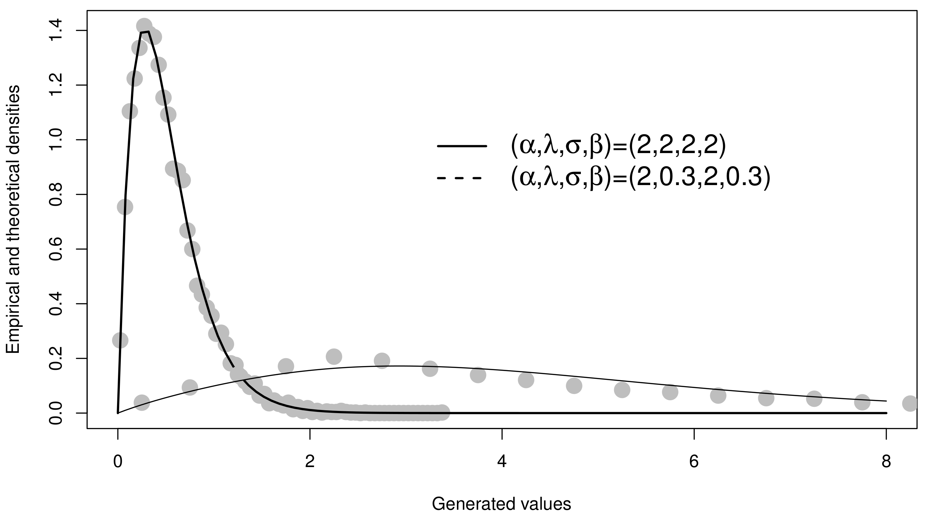
Figure 1 displays two simulated GLL-Exp cases. It is possible to note the Lambert-based RNG (15) works well. It should be emphasized that the acceptance-rejection simulation method is a good alternative when the latter (derived from the inversion method) fails.

Table 2. Simulation study for quantifying bias and MSE of MLEs in several parametric points.

Points	n	Bias (MSE)
		$\widehat{\mathbf{\alpha }}$	$\widehat{\mathbf{\lambda }}$	$\widehat{\mathbf{\sigma }}$	$\widehat{\mathbf{\beta }}$
(2, 2, 2, 2)	25	1.5367 (10.54)	1.239 (16.13)	5.1049 (116.94)	0.5967 (3.24)
	50	0.7668 (2.84)	1.0606 (12.66)	3.6457 (77.04)	0.3628 (0.47)
	100	0.3838 (1.00)	0.8153 (10.07)	1.8592 (30.74)	0.2577 (0.28)
	200	0.2186 (0.45)	0.6925 (7.65)	0.4983 (6.83)	0.1904 (0.17)
(2, 0.3, 2, 0.3)	25	1.3201 (8.26)	0.7664 (4.65)	8.7398 (237.00)	0.3545 (0.71)
	50	0.5266 (1.87)	0.4327 (1.94)	7.51 (191.22)	0.1726 (0.34)
	100	0.2541 (0.67)	0.2858 (0.69)	5.3906 (117.71)	0.0512 (0.14)
	200	0.0342 (0.19)	0.1274 (0.25)	3.1959 (45.99)	−0.021 (0.04)
(1.2, 3, 1.3, 2)	25	0.2989 (0.63)	3.9986 (77.26)	2.9847 (52.37)	3.5303 (36.28)
	50	0.1096 (0.20)	4.4243 (82.09)	1.4924 (23.35)	3.1313 (25.91)
	100	0.0443 (0.09)	4.4327 (80.18)	0.6669 (9.39)	2.5906 (17.67)
	200	0.0154 (0.05)	4.032 (67.12)	0.2413 (4.20)	2.0593 (11.93)

shows the result of the simulation study. In general, estimating $\lambda$ and $\sigma$ was more difficult than estimating $\alpha$ and $\beta$. However, when the sample size was increased, both the MSE and the bias decreased.

10. Applications

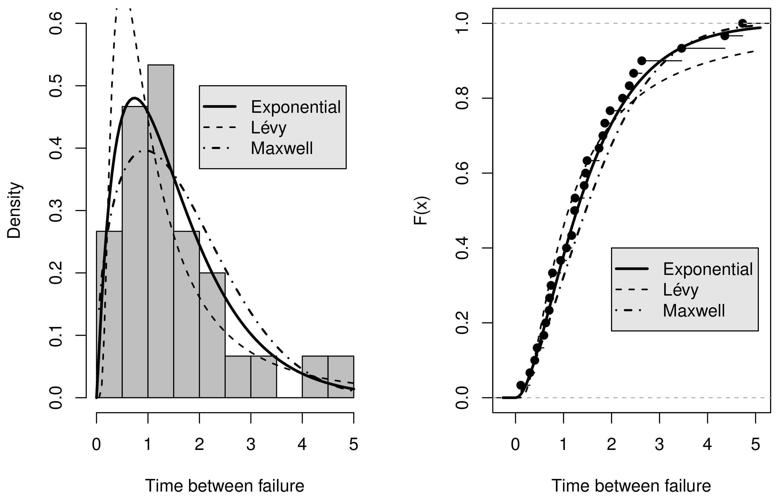
We compare the performance of the generalized log-Lindley-G family having three different baselines as input: exponential, Lévy and Maxwell distributions. The database we used can be found in Hamedani et al., (2017) [37], and it represents the time between failures for repairable items. Figure 2 provides both fits of cdfs and pdfs to the data for the considered models. It is possible to note by visual inspection that the GLL-Exp distribution outperformed the remaining models.

Table 3. Estimates (their standard error) of GLL-G parameters for the repairable data.

GLL-G	Estimates (SEs)
Models	$\widehat{\mathbf{\alpha }}$	$\widehat{\mathbf{\lambda }}$	$\widehat{\mathbf{\sigma }}$	$\widehat{\mathbf{\theta }}$
GLL-Exp	2.18 (0.37)	2.01 (0.71)	1.15 (0.45)	1.12 (0.4)
GLL-L	2.70 (0.27)	3.13 (1.55)	4.49 (0.29)	0.50 (0.24)
GLL-MB	0.41 (0.19)	2.77 (0.41)	3.32 (0.49)	2.99 (0.01)

exhibits MLEs and their associated standard errors (SEs). It is noticeable that these values were well defined in all cases; i.e., asymptotic confidence intervals did not include zero.

Table 4. Goodness-of-fit for the selected baselines.

GLL-G	GoF Measures
Models	AIC	AICc	BIC	K-S
GLL-Exp	87.24	88.84	92.84	0.63
GLL-MB	88.67	90.27	94.28	0.97
GLL-L	94.86	96.46	100.46	0.67

exhibits the results of four goodness-of-fit (GoF) measurements that were employed in this comparison study: Akaike information criterion (AIC), corrected AIC (AICc), Kolmogorov–Smirnov (K-S) and Bayesian information criterion (BIC) statistics. Confirming previous qualitative discussions, the values indicate that the GLL-Exp distribution had the greatest performance.

11. Conclusions

We have established two new families of distributions in this paper named generalized log-Lindley families, which stem from the log-Lindley family. We have obtained several of their mathematical properties, such as expansions for density and cumulative distribution functions, entropies, moment generating functions, entropies and stochastic ordering. Maximum likelihood (ML) estimation procedures have been proposed as well. We have seen through simulation that the ML estimators had behavior aligned with it as expected asymptotically. Finally an application was made in order to illustrate the new family. Results favored the GLL-Exp law relative to the GLL-MB and -L distributions.

References

1. Cordeiro, G.M.; Silva, R.B.; Nascimento, A.D.C. Recent Advances in Lifetime and Reliability Models; Bentham Science Publishers: Sharjah, United Arab Emirates, 2020. [Google Scholar]
2. Lindley, D.V. Fiducial distributions and Bayes’ theorem. J. R. Stat. Soc. Ser. B Methodol. 1958, 20, 102–107. [Google Scholar] [CrossRef]
3. Tomy, L. A retrospective study on Lindley distribution. Biom. Biostat. Int. J. 2018, 7, 163–169. [Google Scholar] [CrossRef] [Green Version]
4. Abouammoh, A.; Kayid, M. A new family of extended Lindley models: Properties, estimation and applications. Mathematics 2020, 8, 2146. [Google Scholar] [CrossRef]
5. Al-Babtain, A.A.; Ahmed, A.H.N.; Afify, A.Z. A new discrete analog of the continuous Lindley distribution, with reliability applications. Entropy 2020, 22, 603. [Google Scholar] [CrossRef] [PubMed]
6. Hafez, E.H.; Riad, F.H.; Mubarak, S.A.M.; Mohamed, M.S. Study on Lindley distribution accelerated life tests: Application and numerical simulation. Symmetry 2020, 12, 2080. [Google Scholar] [CrossRef]
7. Al-Turk, L.I.; Al-Mutairi, N.N. Enhancing reliability predictions by considering learning effects based on one-parameter Lindley distribution. In Proceedings of the 2020 IEEE Asia-Pacific Conference on Computer Science and Data Engineering (CSDE), Gold Coast, QLD, Australia, 16–18 December 2020; pp. 1–7. [Google Scholar]
8. Safari, M.A.M.; Masseran, N.; Majid, M.H. Robust reliability estimation for Lindley distribution—A probability integral transform statistical approach. Mathematics 2020, 8, 1634. [Google Scholar] [CrossRef]
9. Shrahili, M.; Alotaibi, N.; Kumar, D.; Shafay, A.R. Inference on exponentiated power Lindley distribution based on order statistics with application. Complexity 2020, 2020, 4918342. [Google Scholar] [CrossRef]
10. Gomez-Deniz, E.; Sordo, M.; Calderín-Ojeda, E. The log-lindley distribution as an alternative to the beta regression model with applications in insurance. Insur. Math. Econ. 2014, 54, 49–57. [Google Scholar] [CrossRef]
11. Zakerzadeh, H.; Dolati, A. Generalized lindley distribution. J. Math. Ext. 2009, 3, 13–25. [Google Scholar]
12. Jones, M.C. Families of distributions arising from distributions of order statistics. Test 2004, 13, 1–43. [Google Scholar] [CrossRef]
13. Zografos, K.; Balakrishnan, N. On families of beta- and generalized gamma-generated distributions and associated inference. Stat. Methodol. 2009, 6, 344–362. [Google Scholar] [CrossRef]
14. Ristic, M.; Balakrishnan, N. The gamma-exponentiated exponential distribution. J. Stat. Comput. Simul. 2012, 82, 1191–1206. [Google Scholar] [CrossRef]
15. Amini, M.; MirMostafaee, S.M.T.K.; Ahmadi, J. Log-gamma generated families of distributions. Statistics 2013, 1, 1–20. [Google Scholar] [CrossRef]
16. Alzaatreh, A.; Lee, C.; Famoye, F. A new method for generating families of continuous distributions. Metron 2013, 71, 63–79. [Google Scholar] [CrossRef] [Green Version]
17. Jodrá, P.; Jiménez-Gamero, M.D. A note on the log-Lindley distribution. Insur. Math. Econ. 2016, 71, 189–194. [Google Scholar] [CrossRef]
18. Ghitany, M.E.; Atieh, B.; Nadarajah, S. Lindley distribution and its application. Math. Comput. Simul. 2008, 78, 493–506. [Google Scholar] [CrossRef]
19. Ghitany, M.; Al-Mutairi, D.; Balakrishnan, N.; Al-Enezi, L.J. Power lindley distribution and associated inference. Comput. Stat. Data Anal. 2013, 64, 20–33. [Google Scholar] [CrossRef]
20. Sharma, V.; Singh, S.; Singh, U.; Agiwal, V. The inverse lindley distribution: A stress-strength reliability model with application to head and neck cancer data. J. Ind. Prod. Eng. 2015, 32, 162–173. [Google Scholar] [CrossRef]
21. Barco, K.; Mazucheli, J.; Janeiro, V. The inverse power lindley distribution. Commun. Stat. Simul. Comput. 2017, 46, 6308–6323. [Google Scholar] [CrossRef]
22. Asgharzadeh, A.; Nadarajah, S.; Sharafi, F. Generalized inverse lindley distribution with application to danish fire insurance data. Commun. Stat. Theory Methods 2015, 46, 5001–5021. [Google Scholar] [CrossRef]
23. Ramos, P.; Louzada, F. The generalized weighted lindley distribution: Properties, estimation and applications. Cogent Math. 2016, 3, 11. [Google Scholar] [CrossRef]
24. Bhati, D.; Malik, M.; Vaman, H.J. Lindley-exponential distribution: Properties and applications. Metron 2015, 73, 335–357. [Google Scholar] [CrossRef]
25. Grassia, A. On a family of distributions with argument between 0 and 1 obtained by transformation of the gamma and derived compound distributions. Aust. J. Stat. 1977, 19, 108–114. [Google Scholar] [CrossRef]
26. Nadarajah, S.; Kotz, S. The exponentiated type distributions. Acta Appl. Math. 2006, 92, 97–111. [Google Scholar] [CrossRef]
27. Kullback, S. Information Theory and Statistics; Dover Books on Mathematics; Dover Publications: New York, NY, USA, 2012. [Google Scholar]
28. Shannon, C.E. A mathematical theory of communication. Bell Syst. Technol. J. 1948, 27, 379–423. [Google Scholar] [CrossRef] [Green Version]
29. Rényi, A. On measures of entropy and information. In Proceedings of the 4th Berkeley Symposium on Mathematical Statistics and Probability, Berkeley, CA, USA, 20 June–30 July 1961; Volume 1, pp. 547–561. [Google Scholar]
30. Mathai, A.; Haubold, H. On generalized distributions and pathways. Phys. Lett. A 2008, 372, 2109–2113. [Google Scholar] [CrossRef] [Green Version]
31. Nadarajah, S.; Zografos, K. Formulas for Rényi information and related measures for univariate distributions. Inf. Sci. 2003, 155, 119–138. [Google Scholar] [CrossRef]
32. Nadarajah, S.; Zografos, K. Expressions for Rényi and Shannon entropies for bivariate distributions. Inf. Sci. 2005, 170, 173–189. [Google Scholar] [CrossRef]
33. Almanjahie, I.M.; Dar, J.G.; Al-Omari, A.I.; Mir, A. Quantile version of Mathai-Haubold entropy of order statistics. Comput. Model. Eng. Sci. 2021, 128, 907–925. [Google Scholar] [CrossRef]
34. Fashandi, M.; Ahmadi, J. Characterizations of symmetric distributions based on Rényi entropy. Stat. Probab. Lett. 2012, 82, 798–804. [Google Scholar] [CrossRef]
35. Paul, J.; Thomas, P.Y. On some properties of Mathai-Haubold entropy of record values. J. Indian Soc. Probab. Stat. 2019, 20, 31–49. [Google Scholar] [CrossRef]
36. Gradshteyn, I.S.; Ryzhik, I.M. Table of Integrals, Series, and Products, 7th ed.; Elsevier: Amsterdam, The Netherlands, 2007. [Google Scholar]
37. Hamedani, G.G.; Cordeiro, G.M.; Lima, M.C.S.; Nascimento, A.D.C. Some extended classes of distributions: Characterizations and properties. Pak. J. Stat. Oper. Res. 2017, 13, 893. [Google Scholar] [CrossRef] [Green Version]
Figure 1. Estimated and empirical density from simulated data.
Mathematics 09 03108 g001
Figure 2. Estimated and empirical density and cdf of the selected baselines for repairable data.
Mathematics 09 03108 g002