
Categorical Functional Data Analysis. The cfda R Package


Abstract
:1. Introduction
2. Categorical Functional Data Analysis
- and
2.1. The Principal Components
2.2. Optimal Encoding Functions
2.3. Expansion Formulas and Dimension Reduction
- the set of principal components are zero-mean and uncorrelated:
- –
- –
- the set of eigen-processes , which generates the principal components by (7),are zero-mean and of unit total variance.
- the optimal encoding functions, . They generate the eigen-processes by (11),They satisfy the normalization condition (13).
- –
- graphical representation of sample paths of X in (especially for , one obtains a 2-D representation of categorical functional data);
- –
- fit of clustering and regression models with X as explanatory variables;
- –
- outliers or unusual data detection: in the context of real-valued functional data, in [20], the authors propose transformations and algorithms based on the concept of depth function in order to detect outliers. Transforming a real-valued functional variable into a categorical functional one (interval discretisation) and then performing optimal encoding can be an alternative to that proposed in [20].
2.4. Approximation of Optimal Encoding Functions: A Basis Expansion Approach
- The matrix G is the covariance matrix of the random variables , defined as
- The matrix F is defined bywhere is the random variableThus, F is a block diagonal matrix, each block being a square matrix of size corresponding to each x in , .
2.5. Estimation
- the V data set with n rows and columns for the V’s random variables,
- and the U dataset with n rows and Km columns for the U’s random variables, respectively:
- The approximation of optimal encoding functions in a basis of functions is based on the computation of random variables and defined in (22) and (25), respectively. The computation of integrals involved in the definition of these random variables uses the inprod function of the fda R package which, at its turn, calls the function eval.fd. For n and K fixed, this step is the most computational in terms of time resources, and it depends on the number of basis functions, m, considered for the approximation (19). As the computation is performed for every in , parallel computation is performed.
- The F matrix (24) can be singular in some specific situations, namely when there exists an interval and some state x such that . In this case, the hypothesis is not satisfied. For , the operator is degenerated; however, the eigenvalue Equation (5) is still valid. From (12), the optimal encoding function is not defined for . From a computational point of view, if is some element of the basis functions with support in I, then the random variables and are zero-constant and therefore, the row and column corresponding to in the F and G matrices are zero vectors. Thus, the element of the expansion coefficients vector is not defined. Dropping the rows and columns from F and G corresponding to enables solving the eigen-problem in (26). Notice that the constraints (27) are fulfilled.
3. The cfda Package through Examples
3.1. Data
3.1.1. An Example of Real Dataset: Paths of Patients with Severe Infection
- –
- “D”: the patient has not a medical followup,
- –
- “C”: the patient has a medical followup but no treatment,
- –
- “T”: the patient has a medical followup with a treatment, but the infection is not suppressed,
- –
- “S”: the patient has a medical followup with a treatment, and the infection is suppressed.
id time state
 3    0     D
 3    5     D
 9    0     D
 9    1     D
13    0     D
13    7     D
15    0     D
15    4     T
15    7     C
15    8     D
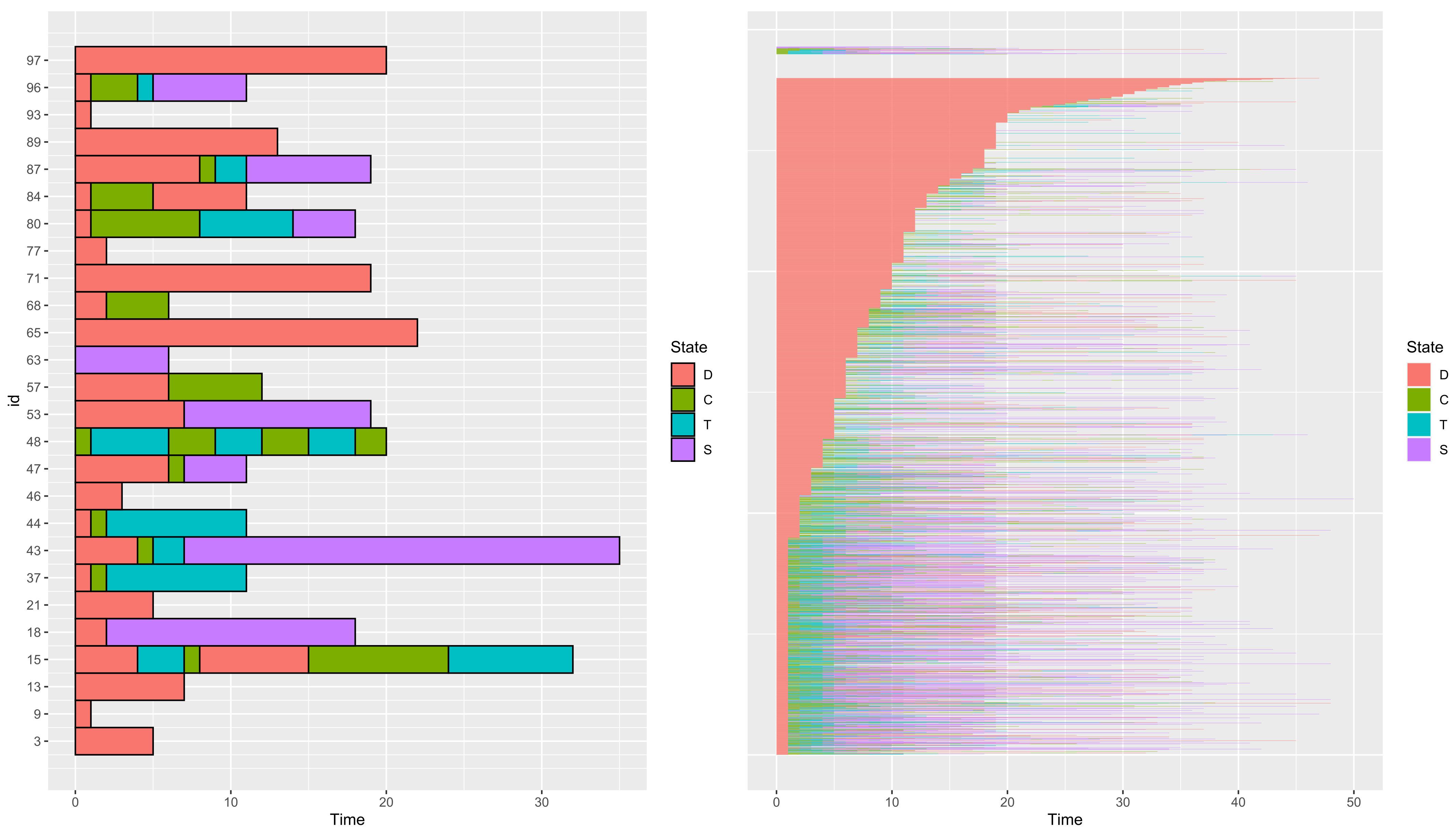
3.1.2. Visualize a Dataset
Number of rows: 10017
Number of individuals: 2929
Time Range: 0--50
Same time start value for all ids: TRUE
Same time end value for all ids: FALSE
Number of states: 4
States:
   D, T, C, S
Number of individuals visiting each state:
   D    C    T    S
2905 1154 1014 1063
- group
- a vector of the length of the number of paths of data containing a variable describing a group structure (if any) of data. Paths from different groups are displayed on different subplots. Paths whose group is coded asNA are ignored.
- addId
- a boolean to add the id of paths on the y-axis.
- addBorder
- a boolean to add the black border around each state.
- sort
- a boolean to sort paths according to the duration of their first state.
- col
- allows users to customize state colors by providing a vector of the same length as the number of state. col is a character (named) vector containing defined color names from R (e.g., c(“red”, “blue”, “darkgreen”)) or RGB colors (e.g., c(“#E41A1C”, “#377EB8”, “#4DAF4A”)).
- nCol
- only when group is used, the number of columns used to display different groups.
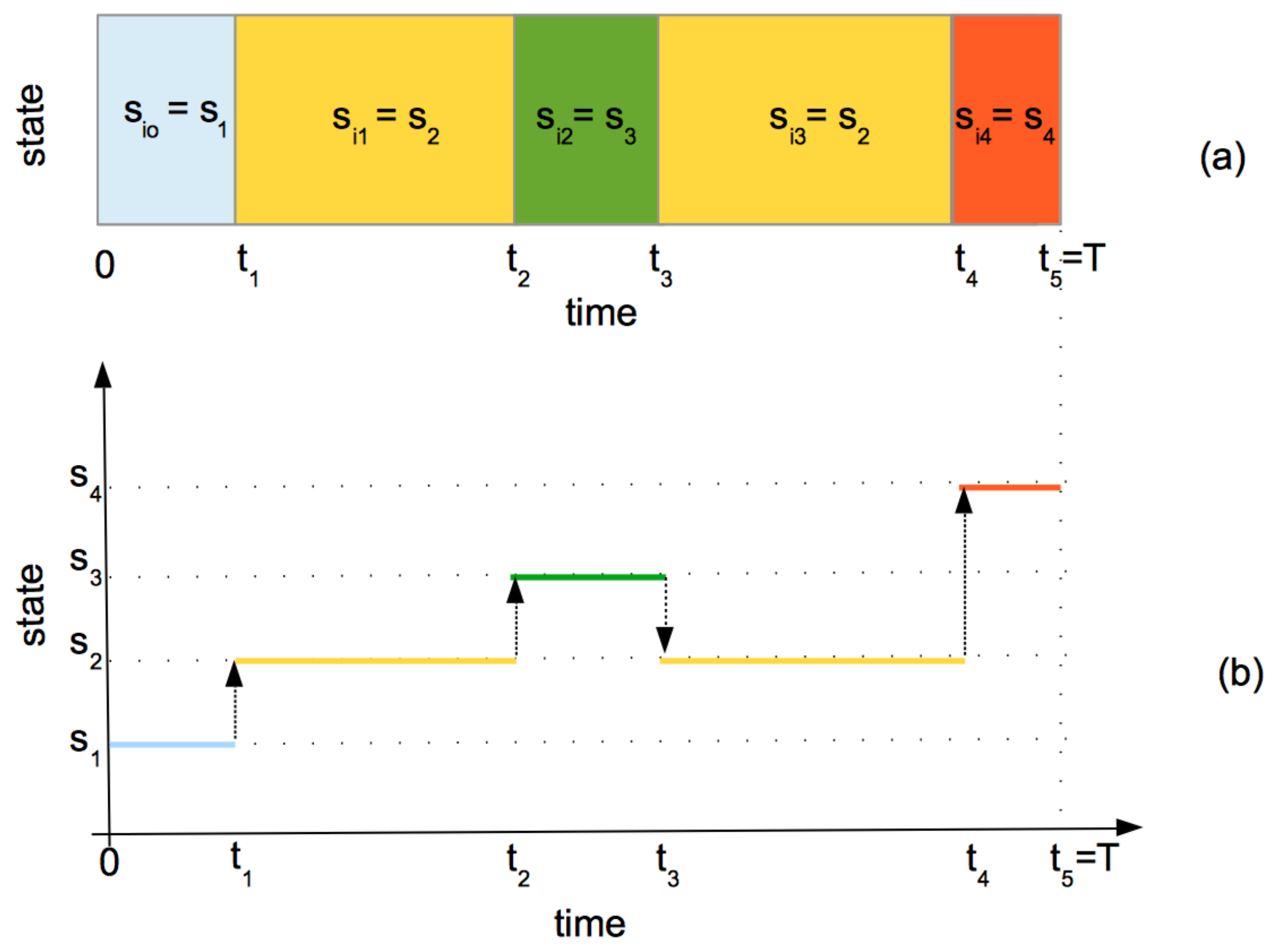
3.1.3. Paths of Same Length T
3 9 13 15 18 21
5 1  7 32 18  5
   id time state
1  15    0     D
2  15    4     T
3  15    7     C
4  15    8     D
5  15   15     C
6  15   18     C
7  18    0     D
8  18    2     S
9  18   18     S
10 43    0     D
3.2. Basic Statistics for Categorical Functional Data
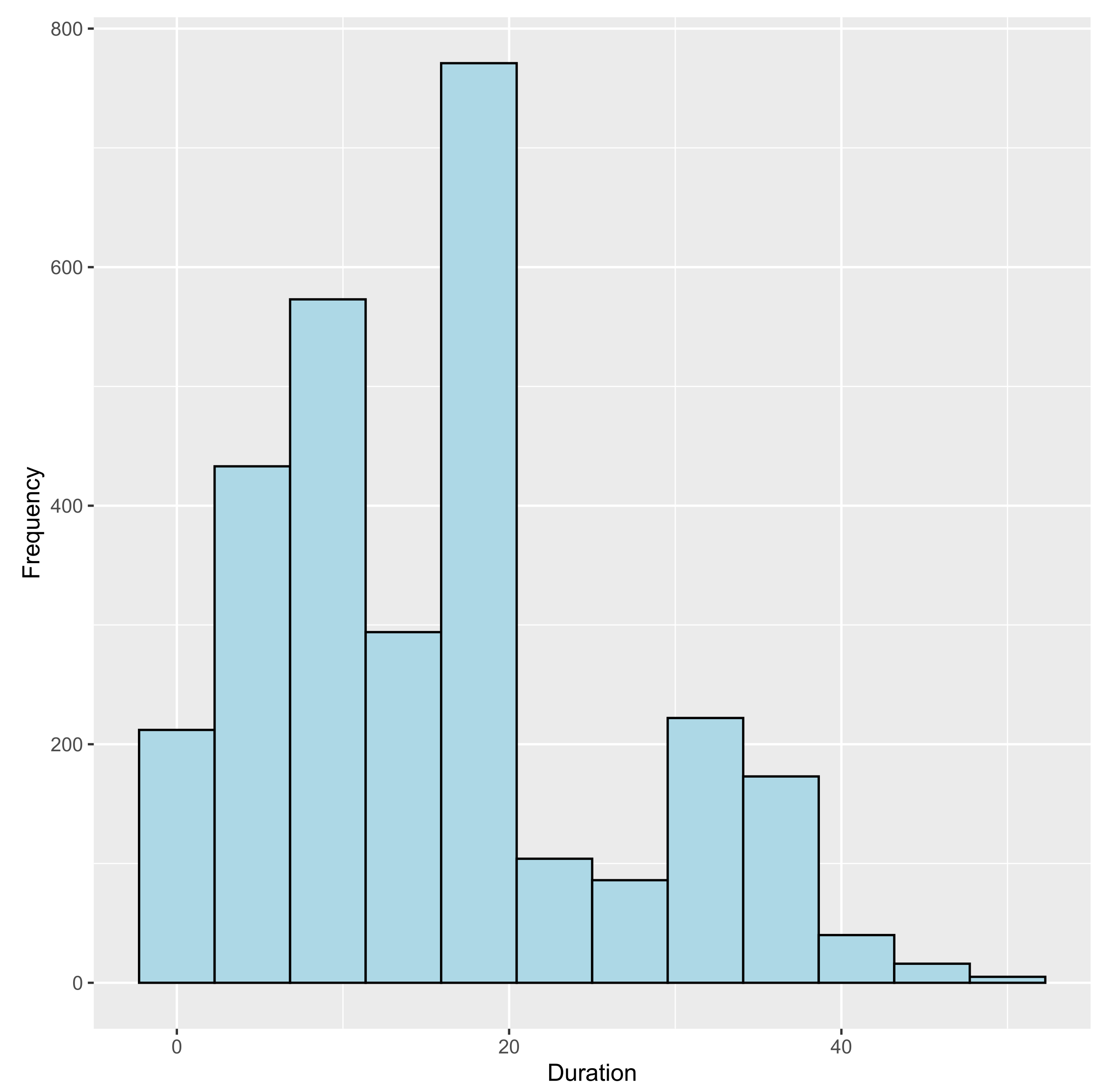
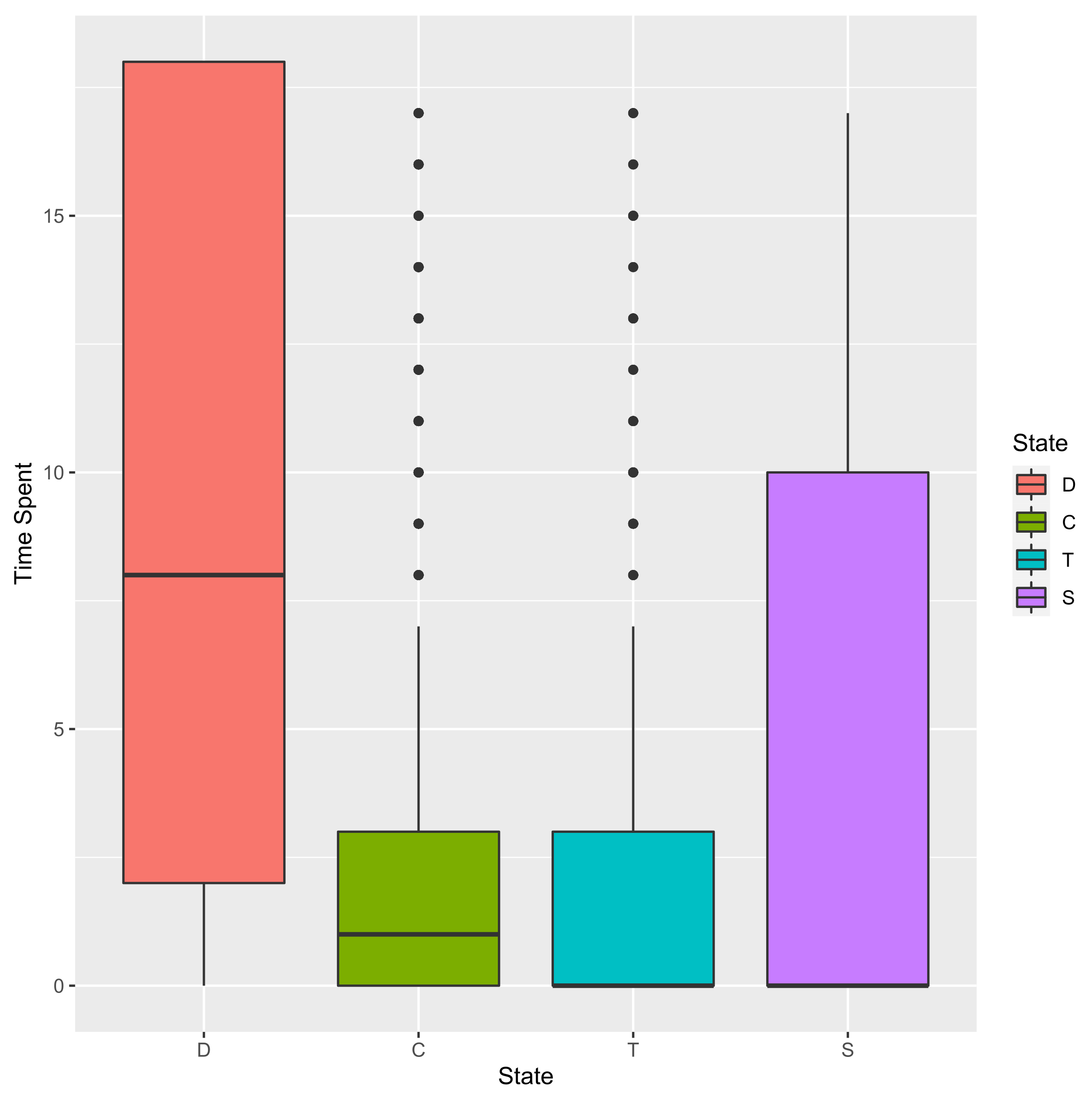
3.2.1. Time Spent in Each State
    D C  T  S
15 11 4  3  0
18  2 0  0 16
43  4 1  2 11
48  0 7 11  0
53  7 0  0 11
65 18 0  0  0
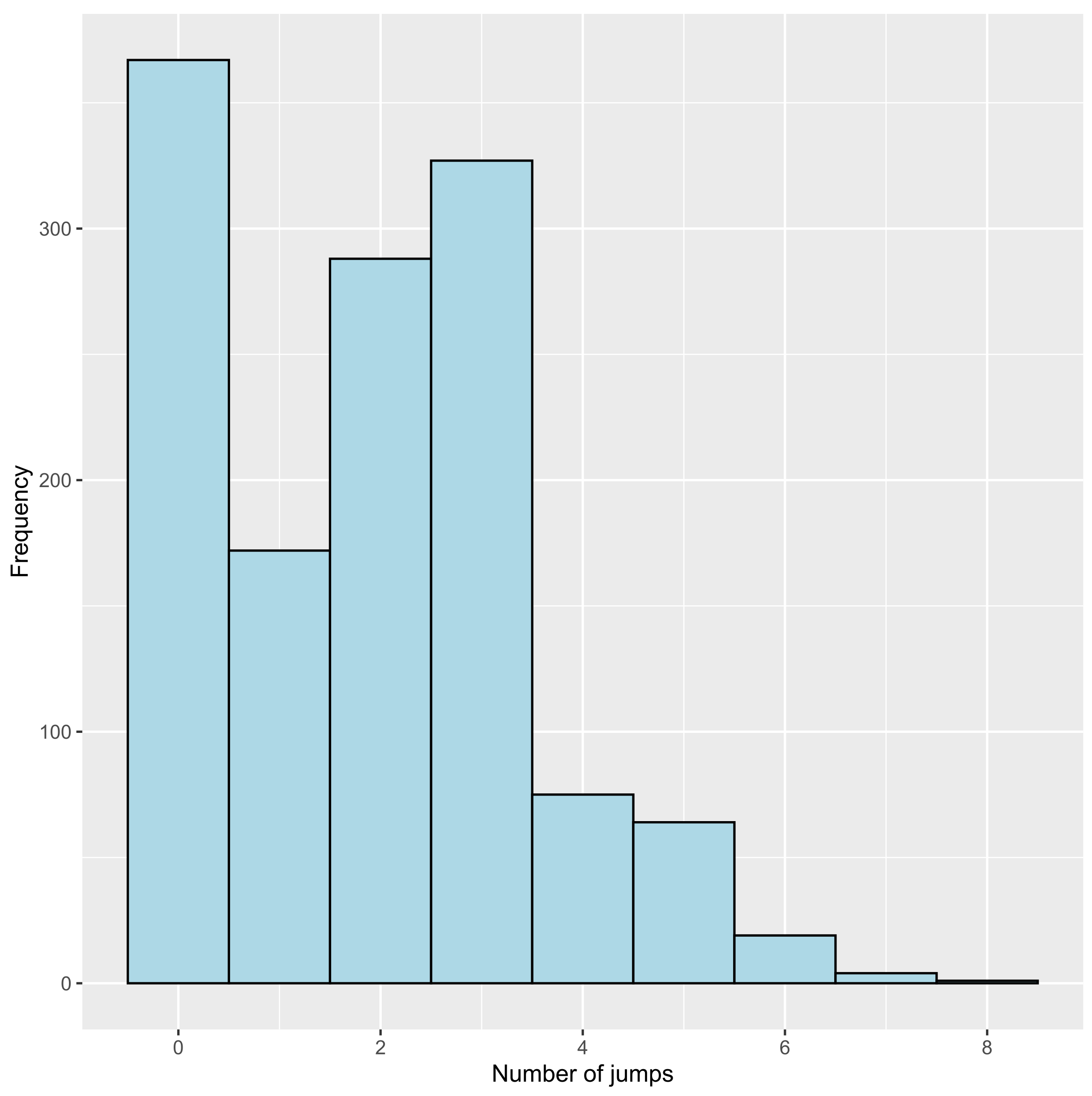
3.2.2. Number of Jumps
15 18 43 48 53 65
 4  1  3  6  1  0
    to
from   D   C   T   S
   D   0 697 253 146
   C 271   0 346  97
   T  16  74   0 461
   S  16  91  31   0
3.2.3. States Distribution over Time
$pt
      0     1     2     3     4     5 ...
D 0.991 0.653 0.596 0.566 0.555 0.552 ...
C 0.008 0.202 0.180 0.166 0.156 0.134 ...
T 0.000 0.099 0.171 0.203 0.159 0.128 ...
S 0.001 0.046 0.053 0.065 0.131 0.185 ...
$t
[1]   0  1  2  3  4  5  6 ...
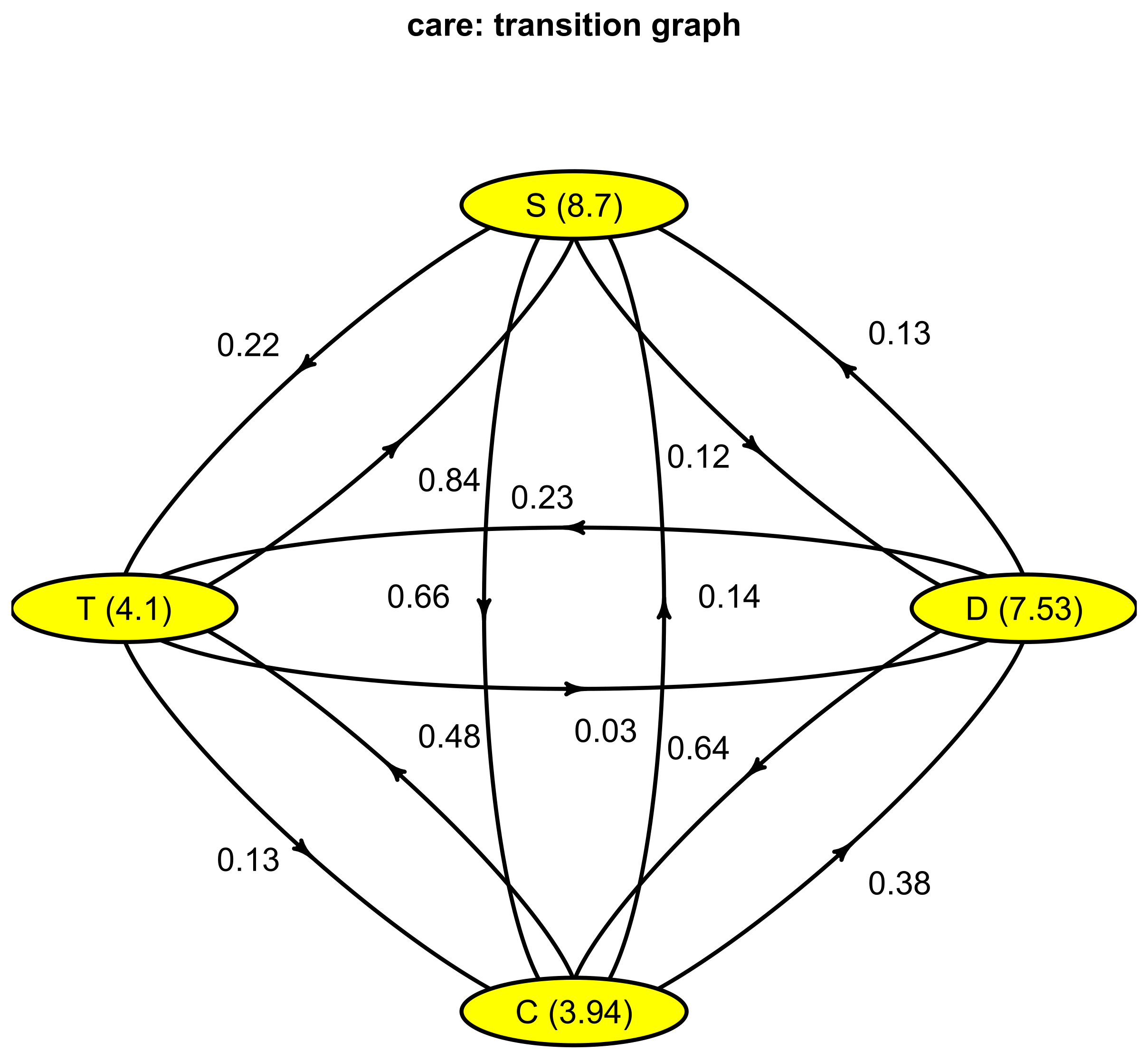
3.2.4. Continuous-Time Markov Chain
$P
    to
from          D          C          T          S
   D 0.00000000 0.63594891 0.23083942 0.13321168
   C 0.37955182 0.00000000 0.48459384 0.13585434
   T 0.02903811 0.13430127 0.00000000 0.83666062
   S 0.11594203 0.65942029 0.22463768~0.00000000
$lambda
        D         C         T         S
0.1328033 0.2538578 0.2438443 0.1149503
attr(,“class”)
[1] “Markov”
3.3. Optimal Encoding
######### Compute encoding #########
Number of individuals: 1317
Number of states: 4
Basis type: bspline
Number of basis functions: 10
Number of cores: 7
---- Compute V matrix:
  |==================================================| 100% elapsed=21 s
DONE in 21.78 s
---- Compute U matrix:
  |==================================================| 100% elapsed=122 s
DONE in 122.42 s
---- Compute encoding:
DONE in 0.13 s
---- Compute Bootstrap Encoding:
**************************************************
DONE in 1.3 s
Run Time: 149.84 s
- eigenvalues
- eigenvalues of the problem (26)
- alpha
- coefficients of the different encoding for each eigenvector (a list of matrices) (26)
- pc
- principal components for each eigenvector
- F
- F matrix (see Equation (24))
- V
- V matrix (see Equation (22))
- G
- covariance matrix of V (see Equation (23))
- basisobj
- basisobj parameter
- bootstrap
- encoding for each bootstrap sample
- varAlpha
- a list containing, covariance matrix of
3.3.1. Plot Functions
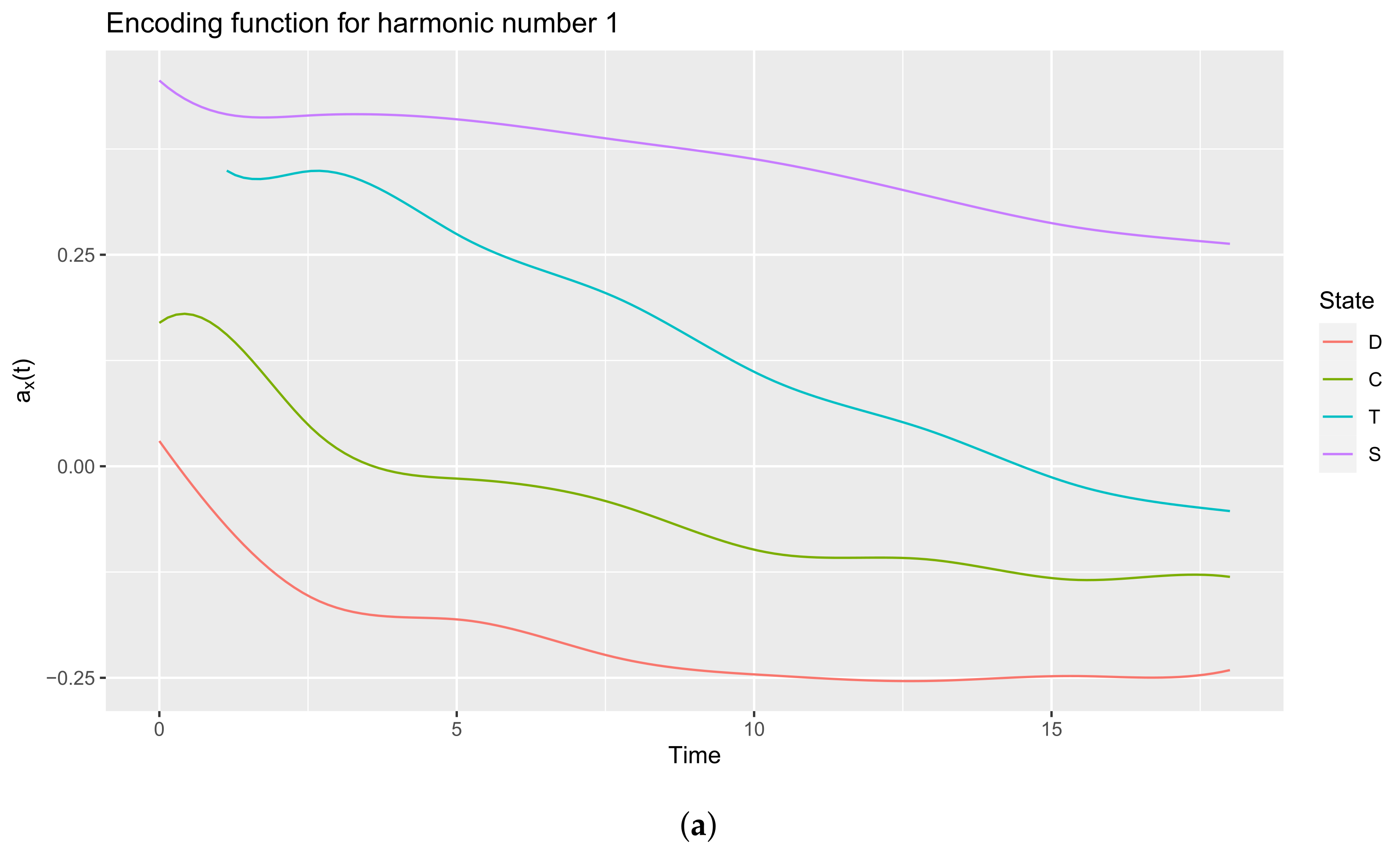
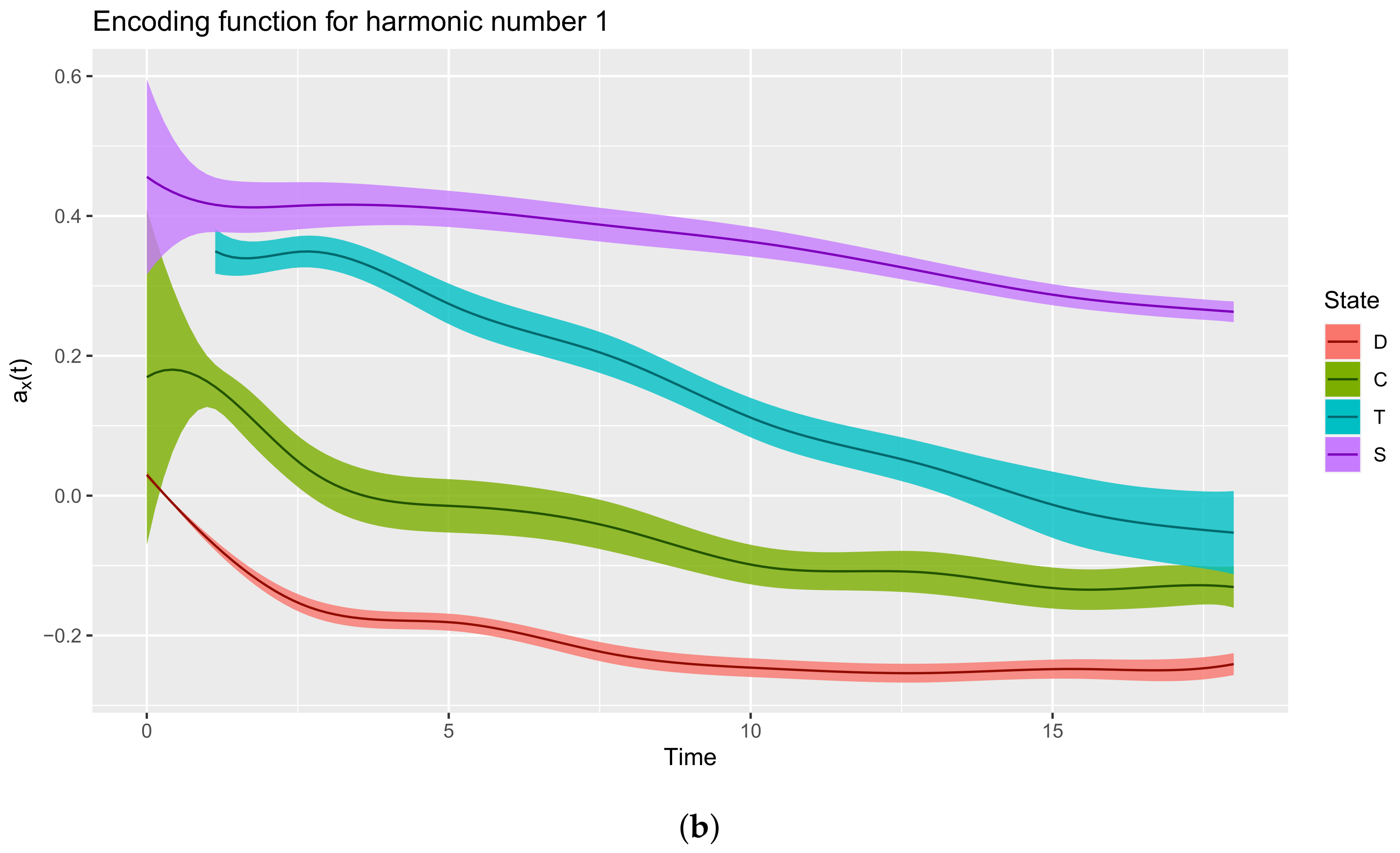
3.3.2. Extract the Encoding Functions
List of 3
$ coefs : num [1:10, 1:4] 0.0299 -0.0543 -0.1965 -0.1645 -0.2371 ...
 ..- attr(*, “dimnames”)=List of 2
 .. ..$ : NULL
 .. ..$ : chr [1:4] “D” “C” “T” “S”
$ basis :List of 10
 ..$ call       : language basisfd(type = type, | __truncated__
 ..$ type       : chr “bspline”
 ..$ rangeval   : num [1:2] 0 18
 ..$ nbasis     : num 10
 ..$ params     : num [1:6] 2.57 5.14 7.71 10.29 12.86 ...
 ..$ dropind    : NULL
 ..$ quadvals   : NULL
 ..$ values     : list()
 ..$ basisvalues: list()
 ..$ names: chr [1:10] “bspl4.1” “bspl4.2” “bspl4.3” “bspl4.4” ...
 ..- attr(*, “class”)= chr “basisfd”
$ fdnames:List of 3
 ..$ args: chr “time”
 ..$ reps: chr [1:4] “reps 1” “reps 2” “reps 3” “reps 4”
 ..$ funs: chr “values”
- attr(*, “class”)= chr “fd”
$x
  [1] 0 1 2 3 4 5 6 7 8 9 10 11 12 13 14 15 16 17~18
$y
                D            C           T         S
 [1,]  0.02986969  0.169492601  0.50380590 0.4559043
 [2,] -0.06073672  0.163315622  0.35643506 0.4180230
 [3,] -0.12970105  0.088328506  0.34225746 0.4126089
 [4,] -0.16758420  0.020411074  0.34651825 0.4159033
 [5,] -0.17812958 -0.007566828  0.31652186 0.4149973
 [6,] -0.18096760 -0.014569119  0.27436391 0.4100582
 [7,] -0.19348217 -0.020533054  0.24249695 0.4020949
 [8,] -0.21335627 -0.032358522  0.21809774 0.3925044
 [9,] -0.23081796 -0.051930578  0.18880144 0.3828197
[10,] -0.24069960 -0.077085840  0.15014660 0.3734934
[11,] -0.24597159 -0.098545473  0.11162958 0.3630747
[12,] -0.25009513 -0.107580629  0.08297660 0.3500902
[13,] -0.25321503 -0.107980977  0.06221397 0.3347482
[14,] -0.25359641 -0.110631333  0.04073503 0.3182122
[15,] -0.25084388 -0.121299335  0.01379572 0.3018281
[16,] -0.24813344 -0.132111070 -0.01301242 0.2873926
[17,] -0.24881502 -0.133707940 -0.03278505 0.2766485
[18,] -0.24943891 -0.128922501 -0.04469775 0.2692082
[19,] -0.24091335 -0.130703127 -0.05297104 0.2629170
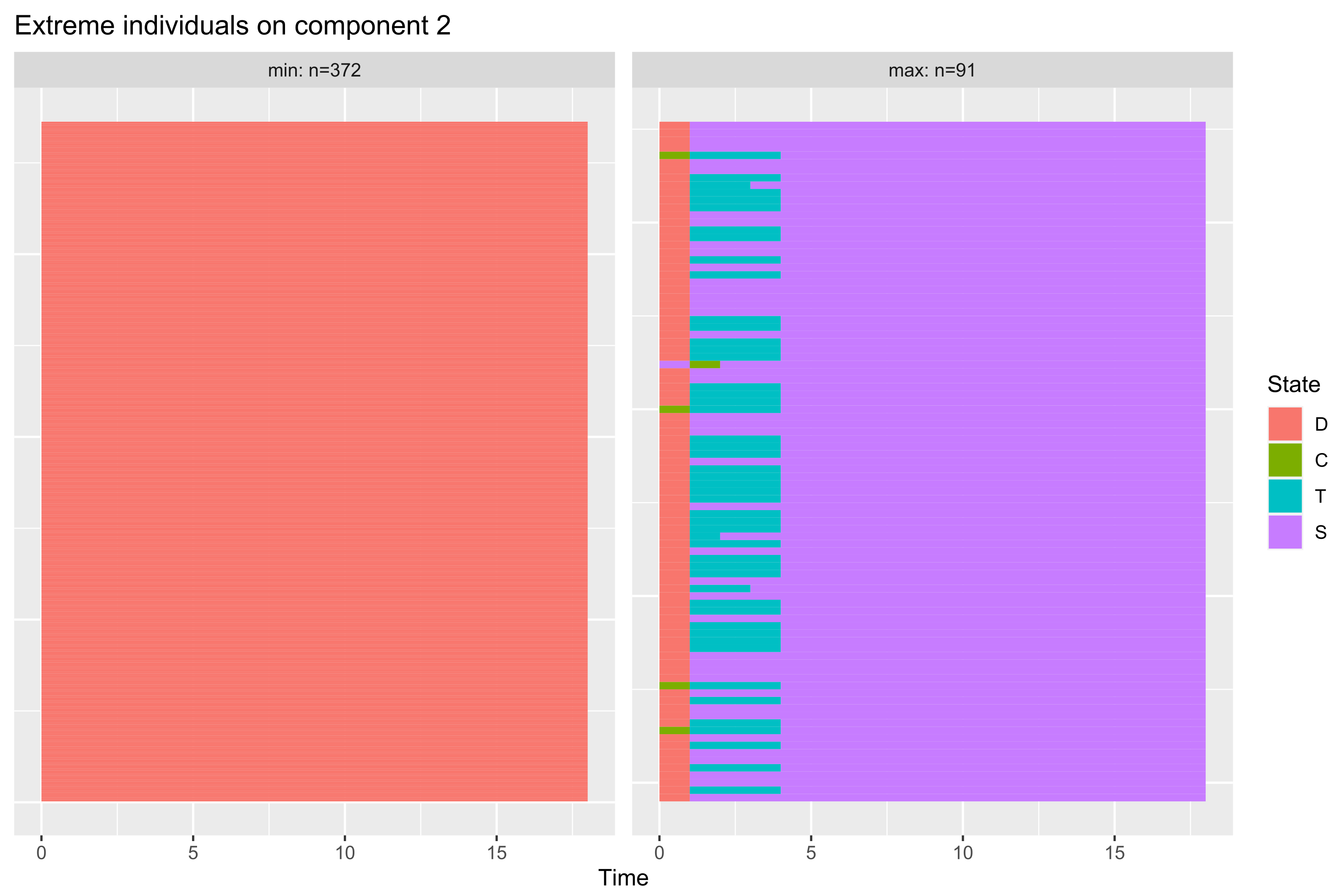
3.3.3. Interpreting the Encoding Functions
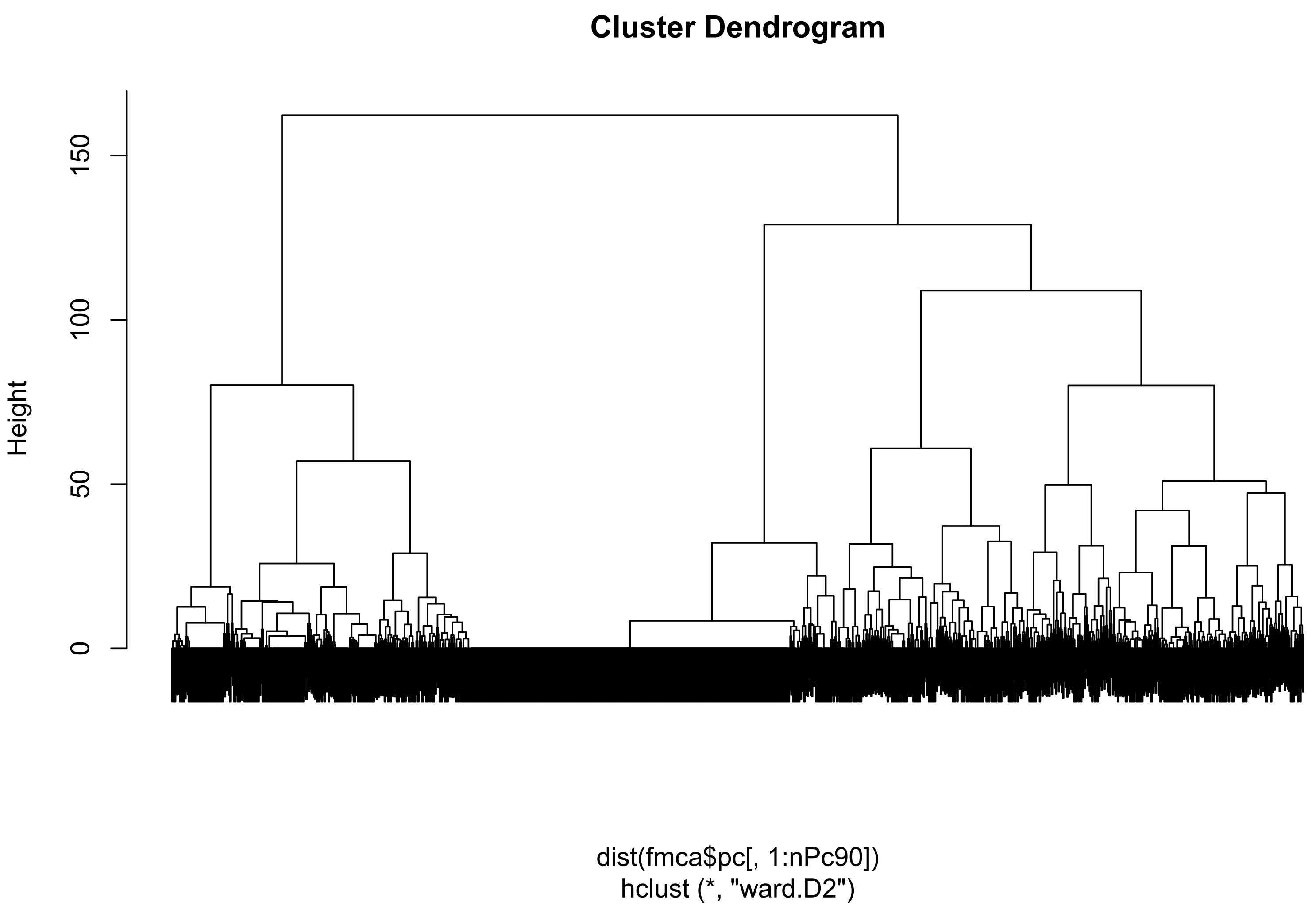
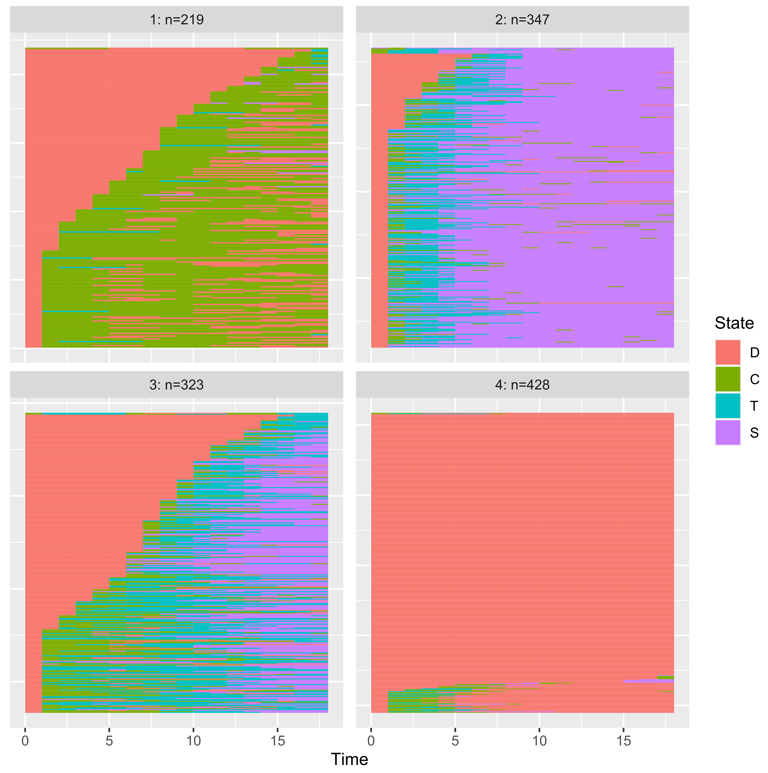
3.3.4. Application to Clustering
4. Simulation Study
4.1. Birth-and-Death Process
- the eigenvalues are given by:
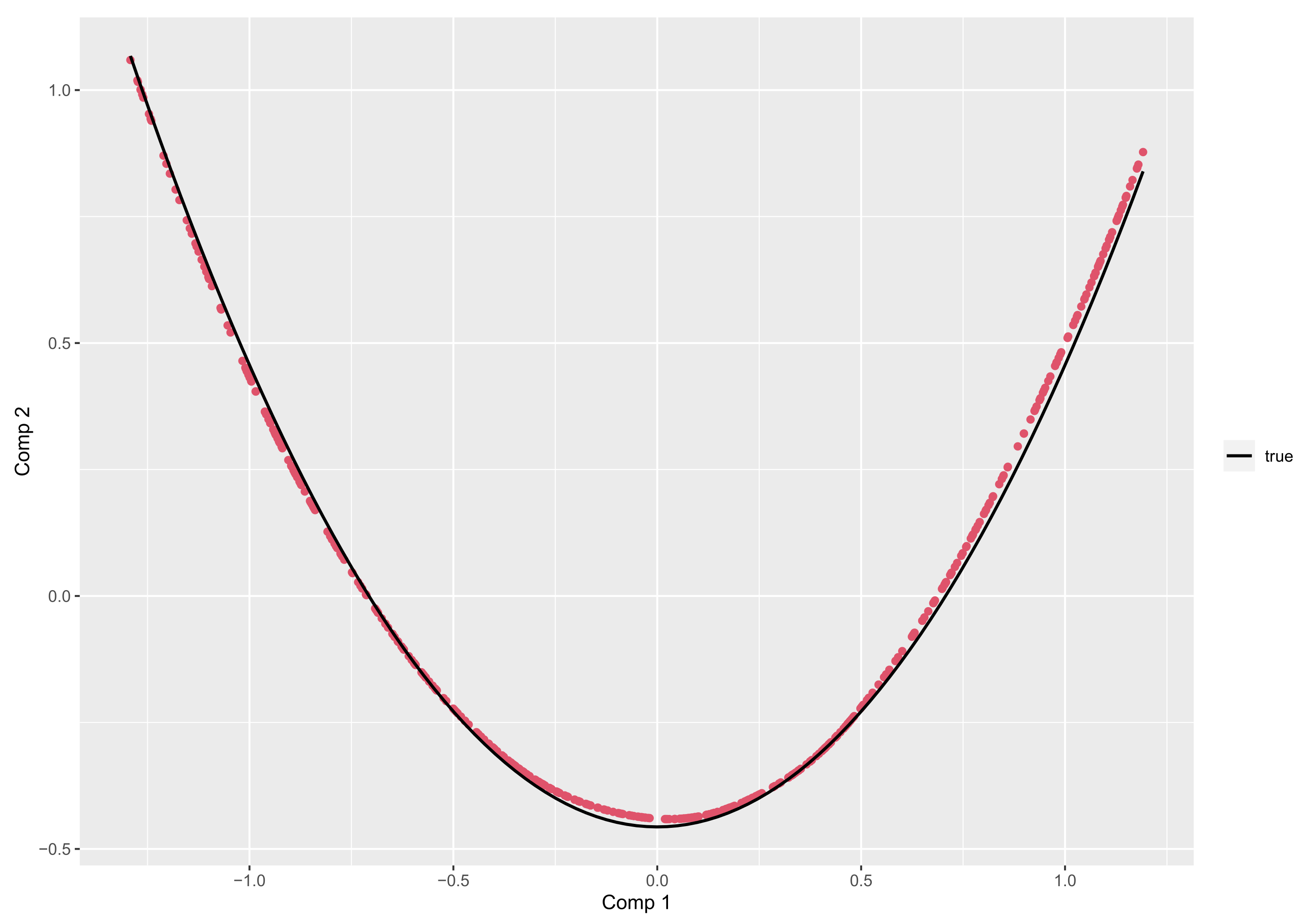
- if is the Legendre polynomials of order n, then the principal components corresponding to , are given, up to a constant, by:In particular, for ,is uniformly distributed on , andObserve that and are linearly uncorrelated but related byshowing some regularity of the 2-D representation of data throughout the plot .
- for , the optimal encoding functions are given by:and
4.2. Results
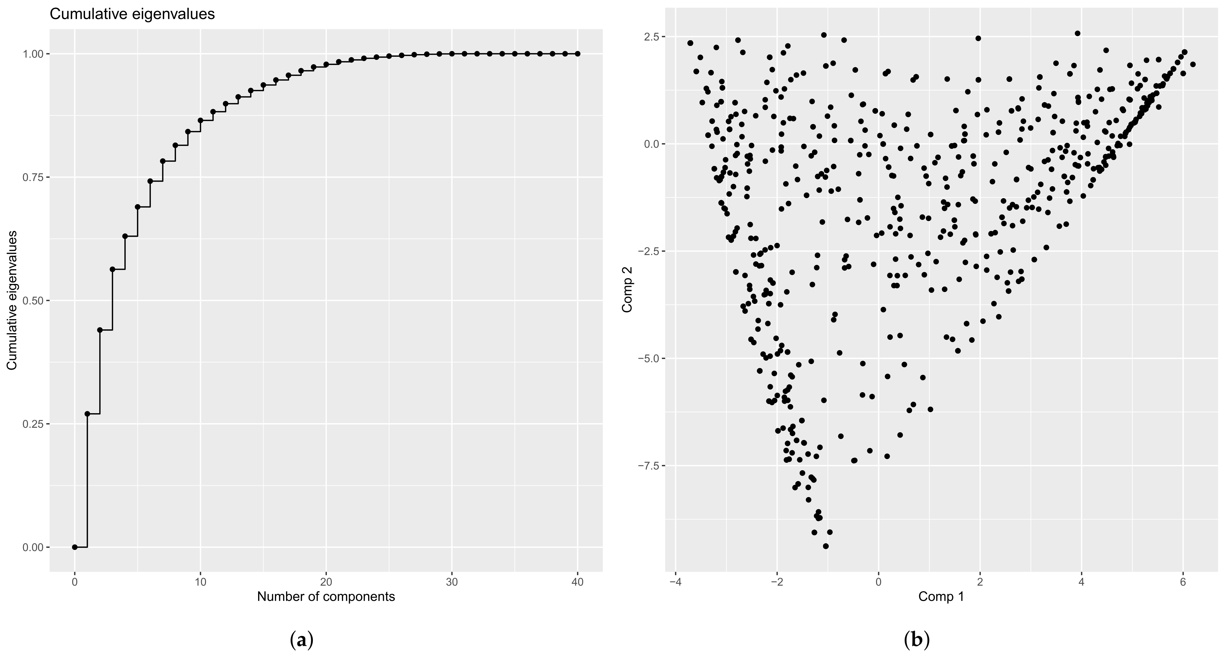
4.2.1. Eigenvalues
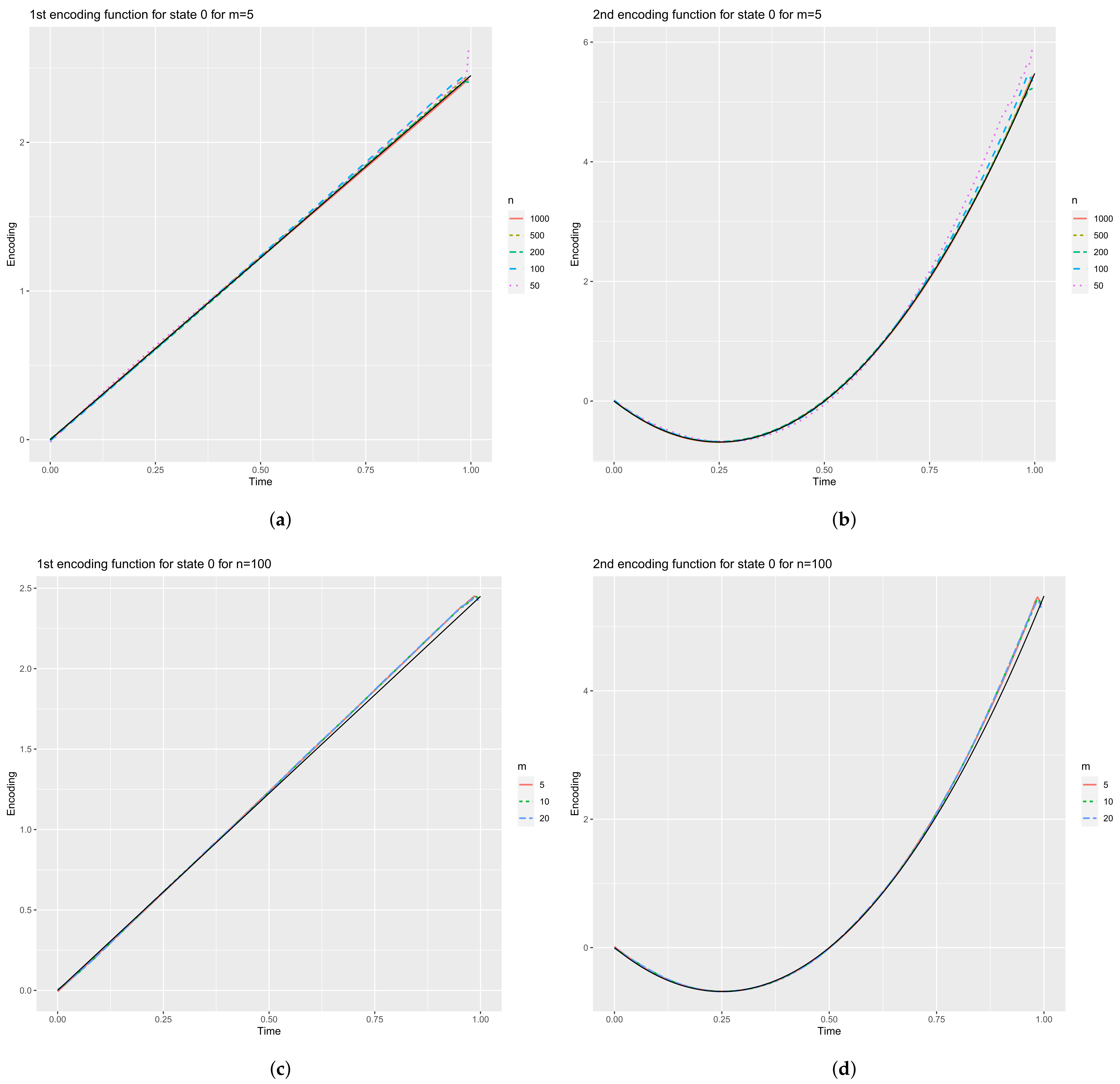
4.2.2. Encoding Functions
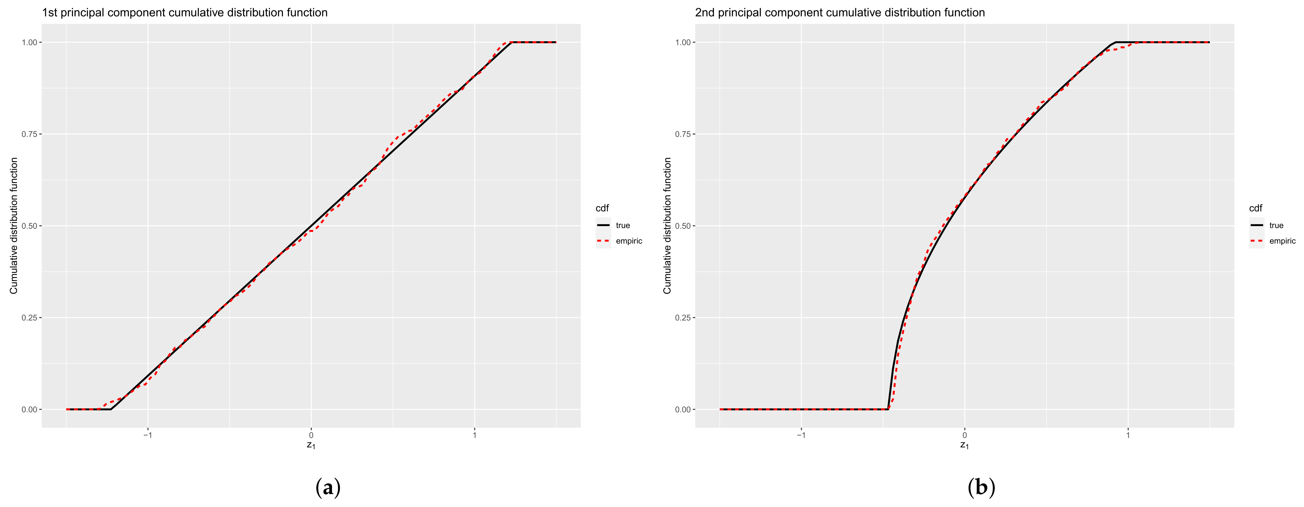
4.2.3. Principal Components
5. Summary and Discussion
Author Contributions
Funding
Institutional Review Board Statement
Informed Consent Statement
Conflicts of Interest
Appendix A
References
- Ramsay, J.; Silverman, B. Functional Data Analysis; Wiley Series in Probability and Statistics; Springer: New York, NY, USA, 2015. [Google Scholar] [CrossRef]
- Ferraty, F.; Vieu, P. Nonparameric Functional Data Analysis. Theory and Practice; Springer: New York, NY, USA, 2006. [Google Scholar] [CrossRef]
- Ramsay, J.O.; Wickham, H.; Graves, S.; Hooker, G. fda: Functional Data Analysis, R Package Version 5.5.1; 2021. Available online: https://cran.r-project.org/package=fda (accessed on 28 November 2021).
- R Core Team. R: A Language and Environment for Statistical Computing; R Foundation for Statistical Computing: Vienna, Austria, 2020. [Google Scholar]
- Jackson, C.H. Multi-State Models for Panel Data: The msm Package for R. J. Stat. Softw. 2011, 38, 1–29. [Google Scholar] [CrossRef] [Green Version]
- Idrovo-Aguirre, B.J.; Lozano, F.J.; Contreras-Reyes, J.E. Prosperity or Real Estate Bubble? Exuberance Probability Index of Real Housing Prices in Chile. Int. J. Financ. Stud. 2021, 9, 51. [Google Scholar] [CrossRef]
- Deville, J.C.; Saporta, G. Correspondence Analysis with an Extension towards Nominal Time Series. J. Econom. 1983, 22, 169–189. [Google Scholar] [CrossRef] [Green Version]
- Deville, J.C. Analyse de Données Chronologiques Qualitatives: Comment Analyser des Calendriers? Ann. De L’INSEE 1982, 45, 45–104. [Google Scholar] [CrossRef]
- Heijden, P.; Teunissen, J.; van Orlé, C. Multiple Correspondence Analysis as a Tool for Quantification or Classification of Career Data. J. Educ. Behav. Stat. 1997, 22, 447–477. [Google Scholar] [CrossRef]
- Boumaza, R. Contribution à l’Étude Descriptive d’une Fonction Aléatoire Qualitative. Ph.D. Thesis, Université Paul Sabatier, Toulouse, France, 1980. [Google Scholar]
- Saporta, G. Méthodes Exploratoires d’Analyse de Données Temporelles; Université Pierre et Marie Curie: Paris, France, 1981. [Google Scholar]
- Preda, C. Analyse Harmonique Qualitative des Processus Markoviens des Sauts Stationnaires. Sci. Ann. Comput. Sci. 1998, 7, 5–18. [Google Scholar]
- Cardot, H.; Lecuelle, G.; Schlich, P.; Visalli, M. Estimating Finite Mixtures of Semi-Markov Chains: An Application to the Segmentation of Temporal Sensory Data. J. R. Stat. Soc. C 2019, 68, 1281–1303. [Google Scholar] [CrossRef]
- Deville, J. Qualitative Harmonic Analysis: An Application to Brownian Motion, Alternative Approach to Time Series Analysis; Publications des Facultés Universitaires Saint-Louis; Universitaires Saint-Louis: Brussels, Belgium, 1984; pp. 1–10. [Google Scholar]
- Nath, R.; Pavur, R. A New Statistic in the One Way Multivariate Analysis of Variance. Comput. Stat. Data Anal. 1985, 2, 297–315. [Google Scholar] [CrossRef]
- Escofier, B. Analyse Factorielle et Distances Répondant au Principe d’Équivalence Distributionnelle. Rev. De Stat. Appliquées 1978, 26, 29–37. [Google Scholar]
- Hotelling, H. Relations Between Two Sets of Variates. Biometrika 1936, 28, 321–377. [Google Scholar] [CrossRef]
- Deville, J.C. Méthodes Statistiques et Numériques de l’Analyse Harmonique. Ann. L’INSEE 1974, 15, 5–101. [Google Scholar] [CrossRef]
- Mercer, J. Functions of Positive and Negative Type and their Connection with the Theory of Integral Equations. Philos. Trans. R. Soc. A 1909, 209, 441–458. [Google Scholar] [CrossRef]
- Dai, W.; Mrkvička, T.; Sun, Y.; Genton, M.G. Functional outlier detection and taxonomy by sequential transformations. Comput. Stat. Data Anal. 2020, 149, 106960. [Google Scholar] [CrossRef] [Green Version]
- Wickham, H. ggplot2: Elegant Graphics for Data Analysis; Springer: New York, NY, USA, 2016. [Google Scholar]
- Solymos, P.; Zawadzki, Z. pbapply: Adding Progress Bar to ’*apply’ Functions, R Package Version 1.4-3; 2020. Available online: https://cran.r-project.org/package=pbapply (accessed on 28 November 2021).
- Gabadinho, A.; Studer, M.; Müller, N.; Bürgin, R.; Fonta, P.A.; Ritschard, G. TraMineR: Trajectory Miner: A Toolbox for Exploring and Rendering Sequences, R Package Version 2.0-13; 2019. Available online: https://cran.r-project.org/package=TraMineR (accessed on 28 November 2021).
- Studer, M. WeightedCluster Library Manual: A Practical Guide to Creating Typologies of Trajectories in the Social Sciences with R. Technical Report, LIVES Working Papers 24. 2013. Available online: https://cran.r-project.org/package=WeightedCluster (accessed on 28 November 2021). [CrossRef]
- Melnykov, V. ClickClust: An R Package for Model-Based Clustering of Categorical Sequences. J. Stat. Softw. 2016, 74, 1–34. [Google Scholar] [CrossRef] [Green Version]
- Scholz, M. R Package clickstream: Analyzing Clickstream Data with Markov Chains. J. Stat. Softw. 2016, 74, 1–17. [Google Scholar] [CrossRef] [Green Version]
- Larmarange, J. Trajectoires de Soins. 2018. Available online: https://larmarange.github.io/analyse-R/trajectoires-de-soins.html (accessed on 28 November 2021).


| m = 5 | ||||||
| true | = 50 | = 100 | = 200 | = 500 | = 1000 | |
| 1 | 0.5000 | 0.5117 (6.4) | 0.5013 (4.4) | 0.5000 (3.1) | 0.5009 (1.8) | 0.5018 (1.5) |
| 2 | 0.1667 | 0.1680 (3.3) | 0.1672 (2.0) | 0.1679 (1.5) | 0.1664 (0.9) | 0.1662 (0.8) |
| 3 | 0.0833 | 0.0824 (1.9) | 0.0835 (1.4) | 0.0834 (0.9) | 0.0835 (0.5) | 0.830 (0.4) |
| 4 | 0.0500 | 0.0455 (1.3) | 0.0490 (0.9) | 0.0494 (0.6) | 0.0492 (0.4) | 0.493 (0.3) |
| 5 | 0.0333 | 0.0184 (0.6) | 0.0205 (0.4) | 0.0211 (0.3) | 0.0215 (0.2) | 0.0216 (0.1) |
| = 10 | ||||||
| true | = 50 | = 100 | = 200 | = 500 | = 1000 | |
| 1 | 0.5000 | 0.5124 (6.4) | 0.5016 (4.3) | 0.5002 (3.1) | 0.5009 (1.8) | 0.5018 (1.5) |
| 2 | 0.1667 | 0.1692 (3.4) | 0.1677 (2.0) | 0.1682 (1.5) | 0.1665 (0.9) | 0.1663 (0.8) |
| 3 | 0.0833 | 0.0841 (2.0) | 0.0843 (1.4) | 0.0839 (0.9) | 0.0837 (0.5) | 0.831 (0.4) |
| 4 | 0.0500 | 0.0486 (1.3) | 0.0510 (0.9) | 0.0508 (0.7) | 0.0501 (0.4) | 0.0501 (0.3) |
| 5 | 0.0333 | 0.0317 (0.8) | 0.0335 (0.6) | 0.0334 (0.4) | 0.0336 (0.2) | 0.0335 (0.2) |
| = 20 | ||||||
| true | = 50 | = 100 | = 200 | = 500 | = 1000 | |
| 1 | 0.5000 | 0.5128 (6.4) | 0.5018 (4.4) | 0.5003 (3.1) | 0.5010 (1.8) | 0.5018 (1.5) |
| 2 | 0.1667 | 0.1699 (3.4) | 0.1681 (2.0) | 0.1683 (1.5) | 0.1666 (0.9) | 0.1663 (0.8) |
| 3 | 0.0833 | 0.0849 (2.0) | 0.0847 (1.4) | 0.0841 (0.9) | 0.0837 (0.5) | 0.0832 (0.4) |
| 4 | 0.0500 | 0.0495 (1.3) | 0.0514 (0.9) | 0.0510 (0.6) | 0.0502 (0.4) | 0.0501 (0.3) |
| 5 | 0.0333 | 0.0327 (0.8) | 0.0340 (0.6) | 0.0337 (0.5) | 0.0337 (0.2) | 0.0335 (0.2) |
Publisher’s Note: MDPI stays neutral with regard to jurisdictional claims in published maps and institutional affiliations. |
© 2021 by the authors. Licensee MDPI, Basel, Switzerland. This article is an open access article distributed under the terms and conditions of the Creative Commons Attribution (CC BY) license (https://creativecommons.org/licenses/by/4.0/).
Share and Cite
Preda, C.; Grimonprez, Q.; Vandewalle, V. Categorical Functional Data Analysis. The cfda R Package. Mathematics 2021, 9, 3074. https://doi.org/10.3390/math9233074
Preda C, Grimonprez Q, Vandewalle V. Categorical Functional Data Analysis. The cfda R Package. Mathematics. 2021; 9(23):3074. https://doi.org/10.3390/math9233074
Chicago/Turabian StylePreda, Cristian, Quentin Grimonprez, and Vincent Vandewalle. 2021. "Categorical Functional Data Analysis. The cfda R Package" Mathematics 9, no. 23: 3074. https://doi.org/10.3390/math9233074
APA StylePreda, C., Grimonprez, Q., & Vandewalle, V. (2021). Categorical Functional Data Analysis. The cfda R Package. Mathematics, 9(23), 3074. https://doi.org/10.3390/math9233074