1. Introduction
The Lindstedt-Poincaré method is a well-known perturbation technique to seek analytic solutions of weakly nonlinear oscillators. Its major essence is expressing the unknown frequency in the powers of small parameters, whose unknown coefficients are determined to avoid secular solutions. There are different perturbation methods [
1], which are popularly applied to solve the nonlinear problems involving small parameters. For weakly nonlinear problems, the modified Lindstedt-Poincaré methods were developed; they can be considered as the extensions of the perturbation method to avoid the secular terms. There are several methods to find the analytic solution, including the Lindstedt-Poincaré method, the Krylov–Bogoliubov–Mitropolsky method, the harmonic balance method, and the multi-time expansions method [
2], which are generally effective for weakly nonlinear systems. Some methods for analyzing the analytic solutions of strongly nonlinear oscillators can be found in [
3], including some modifications of the Lindstedt-Poincaré method [
4,
5,
6].
The determination of period and periodic solution of nonlinear oscillators is an important field in the nonlinear research of physical problems. Some traditional analytical techniques were used to treat nonlinear differential equations, which are usually applied to solve the nonlinear oscillators involving small parameters. If we attempt to obtain an approximate analytical solution of the nonlinear problems, the functional iteration method is a convenient tool. An earlier functional iteration method is the Picard iteration method for nonlinear differential equations. However, it has a major drawback for its slow convergence. To accelerate the convergence, He [
7,
8] has proposed the variational iteration method to render a higher convergence rate for strongly nonlinear problems [
9].
There are many computational methods for finding the periodic solutions of nonlinear oscillators, such as the harmonic balance method [
10,
11,
12], the variational iteration method [
7,
13], the homotopy perturbation method [
14,
15], the parameter-expanding method [
16], the exp-function method [
17], the differential transform method [
18], and the optimally scaled polynomial Fourier series method [
19]. In general, the process to find analytic solutions can be very complicated when the order is increasing. In He’s homotopy perturbation method [
14,
20], the majority is expressing both the analytic solution and a varying frequency in terms of a homotopy parameter, while unknown functions and coefficients are determined by equating each power of the homotopy parameter. Recent works for the homotopy perturbation method applied to solve nonlinear oscillators can be found in [
21,
22]. In addition to the periodic solution, the analytic method is also very important in the bifurcation analysis of dynamic systems [
23,
24].
Traditionally, the Lindstedt-Poincaré method is applied to the original nonlinear differential equation and then a sequence of linear differential equations is derived to determine the analytic solutions. For a higher order analysis, the works in the Lindstedt-Poincaré method become tedious. Here, we first linearize the nonlinear differential equation to a linear one and then apply the modified Lindstedt-Poincaré method to the linearized differential equation. The resulting sequence of the new linear differential equations are simpler than the original ones. In doing so, the computational cost can be reduced, and the work to find the period and analytic periodic solution becomes simpler and easier.
Consider an unforced Duffing oscillator [
2]:
where
is a small parameter.
Let
be a new variable, and then Equation (1) is recast to:
The Lindstedt-Poincaré method [
2] is applied to solve Equation (1) by inserting
and ω of Equation (2) into Equation (3). Equating the coefficients preceding
,
yields:
In addition to the cubic terms , , , and , they also involve the second-order differential terms , , and in the right sides, which might cause a large computational burden in searching the higher order analytic solutions.
An improvement of the Lindstedt-Poincaré method to eliminate the second-order differential terms was performed by He [
5]. Inserting
into Equation (1) up to the third order, one can derive:
The right sides still involve the cubic nonlinear terms , , , and , which might render high computational cost for a higher order analytic solution.
The original Lindstedt-Poincaré method [
2] is more tedious than He’s modified Lindstedt-Poincaré method. The Lindstedt-Poincaré method employed a recursion series of linear ordinary differential equations (ODEs) to determine the analytic solution. How to reduce the cost of computational works is a crucial step for seeking the higher order analytical solution. We will develop a different strategy to improve the above two methods. The novelty is that we can greatly simplify the Lindstedt-Poincaré method to solve the strongly nonlinear oscillators with large vibration amplitude.
2. New Strategy for Second-Order Nonlinear Oscillators
A general second-order nonlinear oscillator is described by:
Suppose that the oscillator vibrates starting from the initial conditions
and
, where
A is a nonzero constant. We begin with a zeroth-order fundamental solution:
where
T = 2π/
ω is the period of the system to be determined, and
and
are the given initial conditions.
Given
in Equation (16), we seek the new analytic solution by solving a linear ODE:
which is a linearization of Equation (15) around
and
is a weight parameter. Equation (17) is a periodic system equipped with a fundamental frequency
ω to be determined, and then we take:
In terms of the new variable
θ, we can replace
in Equation (17) by
and write:
where the prime denotes the differential with respect to
θ, so that Equation (17) becomes:
Before deriving the analytic solution for Equation (1), we discuss its linearization. For a single nonlinear equation
, the Newton technique is derived by giving an initial guess
and solving a linearized equation
to approximate the solution of
, which results in the famous Newton iterative method:
Similarly, given a zeroth-order fundamental solution
in Equation (16) for the function
, we can linearize the cubic term
in Equation (1) around
by
which can be arranged to:
Equation (23) is obtained from Equation (1) by Newtonian linearization. Here, instead of Newtonian linearization, we propose a new linearization technique. Notice that Equation (1) is equivalent to the following two equations:
where
is a weight factor. If we replace
on the left side with
as a linearization, and
on the right side with
, we can obtain:
Taking , Equation (24) coincides with Equation (23). Therefore, the Newtonian linearization is a special case of Equation (24) for the Duffing equation.
After inserting
into Equation (24), in terms of
θ and dividing both sides by
, this leads to a periodically varying coefficient linear differential equation:
where
Equation (25) is Mathieu’s equation with periodic forcing terms on the right side [
25].
There are different techniques to solve the Mathieu equation, e.g., the method of strained parameters, Whittaker’s method, the method of multiple scales, the method of averaging [
26], the harmonic balance method [
27], and the analytic method [
28].
Here, we develop a linearized Lindstedt-Poincaré method to seek the higher order analytic solutions of Equation (1) through Equation (25). When
, one can refer [
1] for solving Equation (25) by using the method of strained coordinates.
3. A Linearized Lindstedt-Poincaré Method
Now, we use some examples to show how to solve Equation (19) by a linearized Lindstedt-Poincaré method to determine the approximate analytic solutions.
Example 1. To explore the idea for finding analytic solution, we begin with [2]: This differential equation is used to model the free vibration of an eardrum and also in the ship rolling vibration [
29].
By applying the Lindstedt-Poincaré method [
2] to find the analytic solution of Equation (27), the starting point is:
where
and
ω is to be determined. Let
Inserting them into Equation (28) and equating the coefficients preceding
,
and
, we can derive:
For comparison purposes, we write the Lindstedt-Poincaré solution given in [
2]:
where
There are two shortcomings in Equations (31)–(33). In each stage to find , by solving the second-order differential equation, it involves the second-order differentials of , and the nonlinear terms appear. When highly nonlinear problem is encountered, the differentials of and the nonlinear terms are not easily computed, and the process would become complicated. Below, we develop a simpler linearized Lindstedt-Poincaré method to overcome these difficulties.
Given a zeroth-order
of the function
in Equation (27), we have
which can be arranged to
It is a special case of
with
.
For this example, inserting
into Equation (38), we need to solve
which in terms of
becomes
where
Later, we use the first equation to determine the frequency
ω, so it may be called the frequency equation. Inserting Equation (42) into Equation (40) and equating the coefficients preceding
,
and
, we can derive:
Inserting
into Equations (44) and (45) results in:
To avoid the secular terms appeared in
and
, we must take
Through some manipulations, we can derive:
Finally, the second-order analytic solution of Equation (27) is
The value of
ω is solved from Equations (41), (42), and (48) as
We show the cases with different
, where the maximum error within one period for Equation (34) is compared with that computed by the fourth-order Runge-Kutta method (RK4) applied to Equation (27) within
. Similarly, the maximum error within one period for Equation (51) with
listed in
Table 1 is compared with that computed by the RK4 within
T = 2π/
ω. It can be seen that the present ME is smaller than the ME obtained by the Lindstedt-Poincaré method for all
.
Example 2. Consider [2]:where is a small parameter. It permits a periodic solution if is not too large. In terms of
θ, Equation (53) becomes
Then, we decompose it to
and linearize it around
to a linear differential equation for
:
where
is used. For this example, we solve
where
Inserting Equation (42) into Equation (54), we can derive:
To avoid the secular terms appearing in
and
, we can take:
Through some manipulations, we can derive the second-order analytic solution as:
From Equations (55), (59) and (42), the frequency is derived as:
For the sake of comparison, we write the asymptotic solution given in [
2]:
where
In
Table 2, we compare the ME1 for Equation (60) with different
values listed in the table and ME2 for Equation (62) with different
values. The present method is simpler and more accurate than that obtained from Equation (62).
Example 3. For the Duffing equation, inserting Equation (42) into Equation (25) and equating the coefficients preceding , k = 0, 1, 2, 3, renders: Upon comparing Equation (67) to Equations (8) and (14), the present method can save much computational cost, which is merely with three linear terms on the right-hand side.
Inserting Equation (16) into Equations (65) and (66) up to the second order, we can further derive:
To avoid the secular terms appeared in
and
, we must take
Through some manipulations, we can derive the second-order analytic solution as
where
is solved from the following frequency equation as shown by the first equation in Equation (42):
Here, we write the asymptotic solution given in [
2]:
where
In
Table 3, we compare the maximum errors for Equation (71) with
and
A = 1, and for Equation (74) with different
. The accuracy of the present method is much better, and the formulations are simpler. For Equation (1), the exact
ω is given by
whose value is obtained by applying the three-point Gaussian quadrature to the integral term. In
Table 3, we compare
ω obtained from Equations (75), (72), and (76). The value
ω obtained by the present method is more accurate than that obtained by Equation (75). Even up to
, the present results are sufficient; however, the Lindstedt-Poincaré method fails to offer reasonable results for the case with strong nonlinearity.
For the Duffing equation, we compare the frequencies obtained from Equations (72) and (75) to the exact ones for different
in
Figure 1, showing that the present ones almost coincide with that of the exact frequencies obtained from Equation (76) in all values of
. However, when
, the frequencies obtained from Equation (75) are gradually under-estimated with a large discrepancy.
For complicated oscillators, He’s frequency–amplitude formulations [
30,
31,
32,
33,
34] were frequently employed to estimate the frequency of free vibration. For example, for the Duffing oscillator, it reads as:
Here, we take the best value
, and the results are displayed in
Table 3. We can observe that Formula (72) is more accurate than Formula (77).
Example 4. Consider a zero-spring constant Duffing oscillator [5]: As mentioned by He [
5], the standard Lindstedt-Poincaré method cannot be applicable to solve this problem.
The governing equations are still given by Equations (25) and (26), but with a new
The second-order analytic solution is still given by Equation (71), but with a new frequency:
Here, we take again for the linearization of in Equation (78) around .
In
Table 4, we compare the maximum errors with different
and compare
ω obtained from Equation (80) with
A = 1 to the exact one:
Example 5. We apply the linearized Lindstedt-Poincaré method to [5]:which is recast to In terms of
θ, Equation (83) changes to
We decompose it to
which is linearized around
to
where
is used.
Therefore, around the zeroth-order fundamental solution (16), Equation (83) is linearized into a forced Mathieu’s Equation (25) with:
The second-order analytic solution is still given by Equation (71), but with a new frequency:
In
Table 5, we compare the maximum errors with different
A values and compare
ω obtained from Equation (85) with
to the exact one:
We take , rendering ω in Equation (85) close to that in Equation (86).
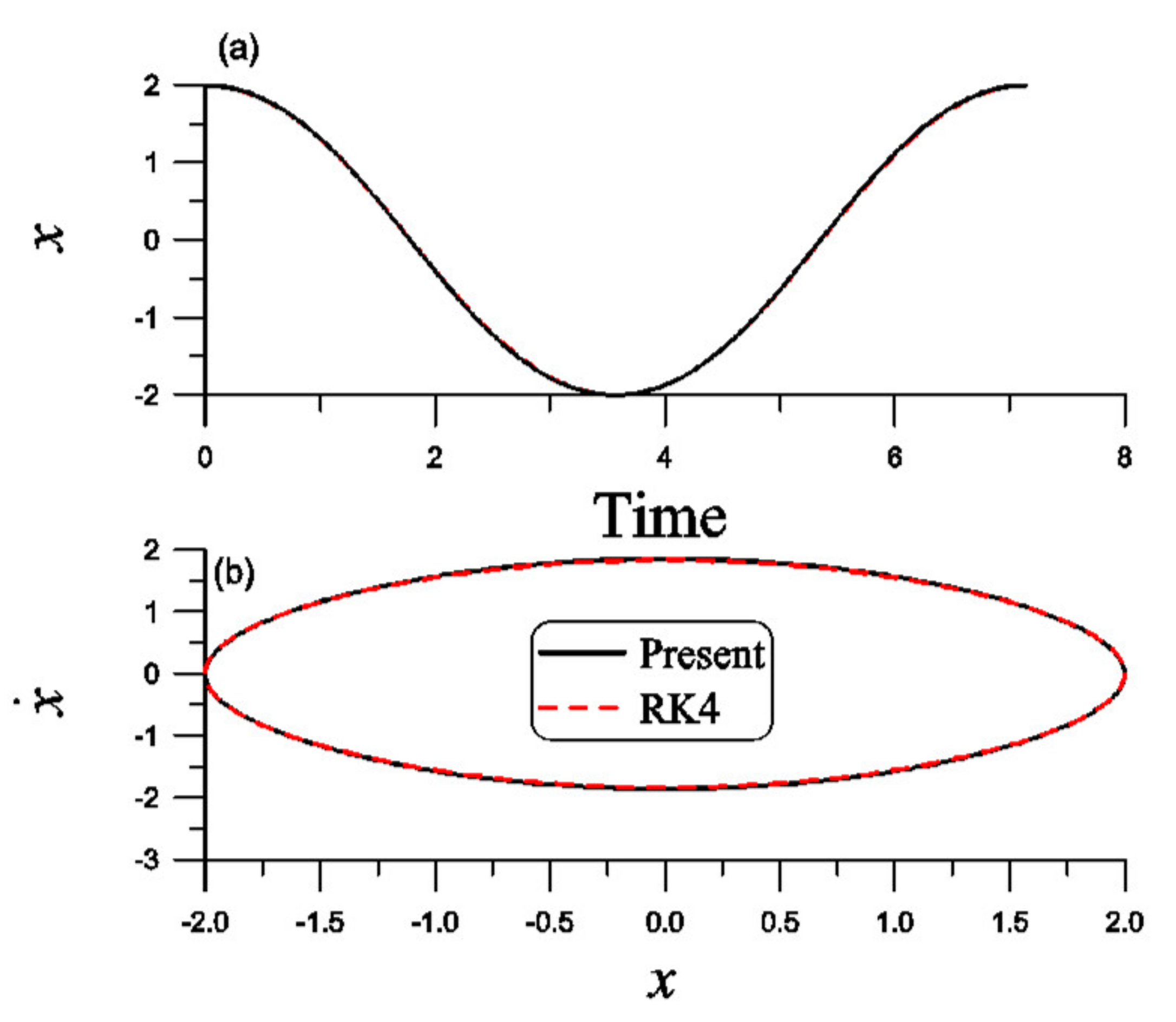
We fix
,
A = 2, and compare the analytic solution (71) to that computed by the RK4 within one period. As shown in
Figure 2a, the solution obtained from Equation (71) is close to the one obtained by the RK4 to integrate Equation (82) with the initial conditions
,
, where the error is smaller than
. The periodic orbit is shown in
Figure 2b.
Example 6. For the van der Pol oscillator [2]:we consider its linearization by Around the zeroth-order solution,
we can recast Equation (88) to
where
Inserting Equation (42) into Equation (90), we can derive:
To avoid the secular terms appeared in
and
, we must take:
where
Through some manipulations, we can derive the second-order analytic solution as:
where
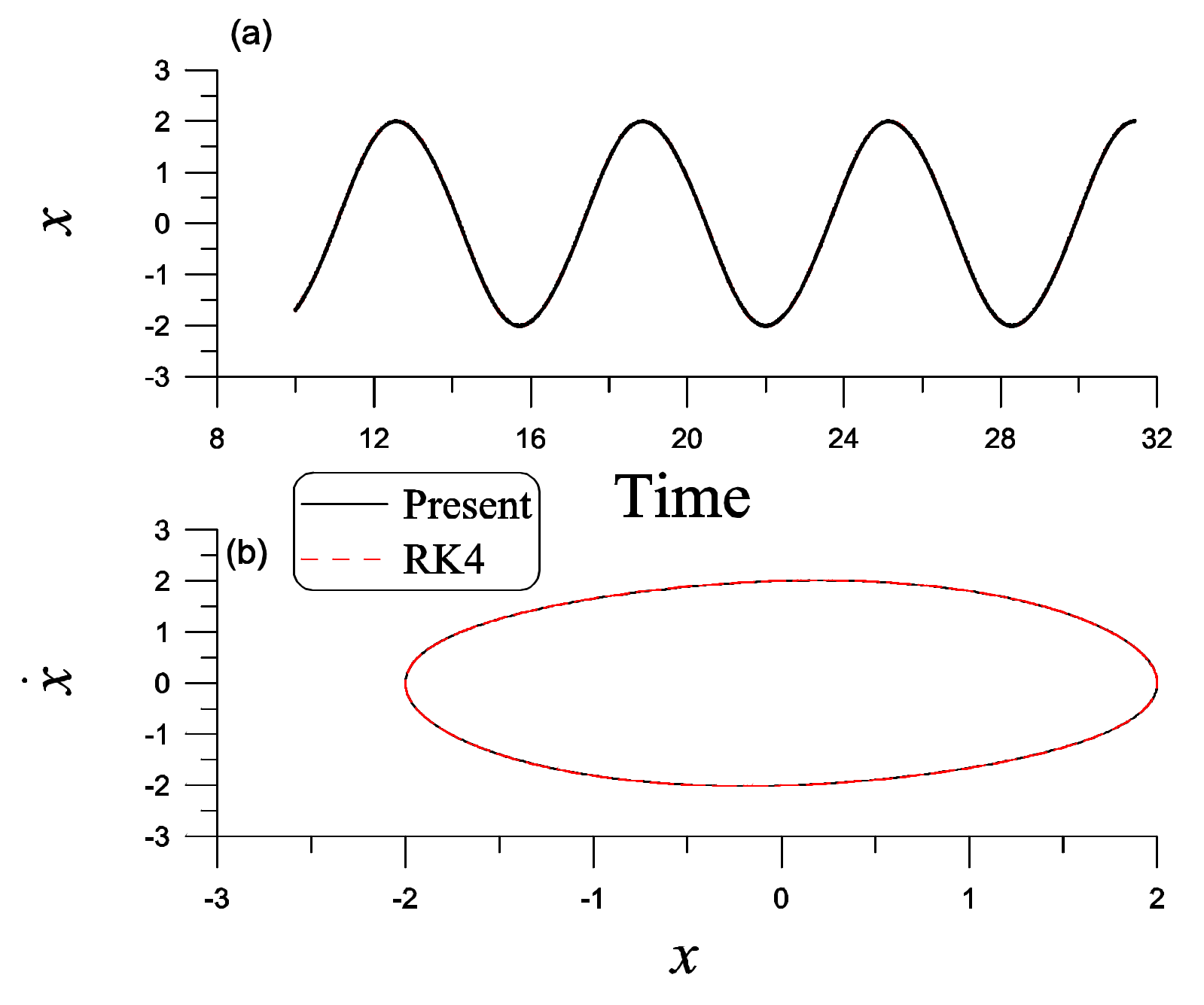
We fix
,
, and compare the analytic solution (97) to that computed by the RK4 up to the steady state with time
. As shown in
Figure 3a, the solution obtained from Equation (97) is close to the one obtained by the RK4 to integrate Equation (87) with initial conditions
,
, where the error is smaller than
. The limit cycle is shown in
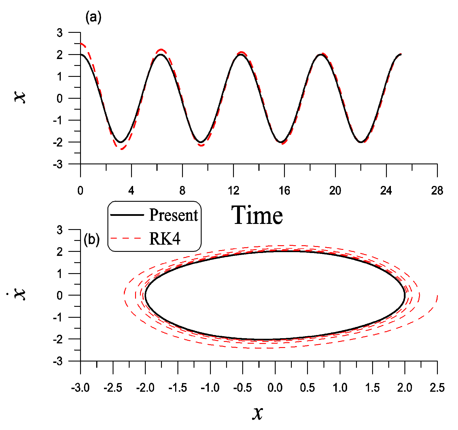
Figure 3b. If we start from an initial value with
A = 2.5, as shown in
Figure 4, the RK4 solution approaches the solution obtained from Equation (97), which is a limit cycle. The maximum errors within one period are listed in
Table 6 with different
values.
Example 7. For the Duffing equation, we consider:which is more difficult than Example 3. The fundamental solution satisfying
and
is:
After inserting
into Equation (24) in terms of
θ and dividing both sides by
, we obtain a periodically varying coefficient linear differential equation:
where
Inserting Equation (42) into Equation (101) and equating the coefficients preceding
,
renders:
To avoid the secular terms appeared in
and
, we must take
Through some manipulations, we can derive the second-order analytic solution as:
where
In
Table 7, we compare the maximum errors for Equation (107) with
,
B = 1, and with different
values. The value
ω obtained by the present method is also listed.
Remark 1. As pointed out in [22,35], the traditional perturbation method contains the shortcoming that it is not useful for the Duffing oscillator if a linear damping term is included. The present method can treat a quite general nonlinear oscillator in Equation (15), which also does not contain a linear damping term. Examples 1 and 3–7 are special cases of Equation (15); however, Example 2 with a nonlinear damping term is not a special case of Equation (15). After inserting into Equation (19), we can derive a linearized differential equation of the Hill type. Then, using the present method, a sequence of linear differential equations can be obtained, which are used to determine the analytic solution. Indeed, the present linearization technique may be applied to general nonlinear vibration systems. 


