Fuzzy Branch-and-Bound Algorithm with OWA Operators in the Case of Consumer Decision Making

Abstract

The ordered weighted averaging (OWA) operator is one of the most used techniques in the operator’s aggregation procedure. This paper proposes a new assignment algorithm by using the OWA operator and different extensions of it in the Branch-and-bound algorithm. The process is based on the use of the ordered weighted average distance operator (OWAD) and the induced OWAD operator (IOWAD). We present it as the Branch-and-bound algorithm with the OWAD operator (BBAOWAD) and the Branch-and-bound algorithm with the IOWAD operator (BBAIOWAD). The main advantage of this approach is that we can obtain more detailed information by obtaining a parameterized family of aggregation operators. The application of the new algorithm is developed in a consumer decision-making model in the city of Barcelona regarding the selection of groceries by districts that best suit their needs. We rely on the opinion of local commerce experts in the city. The key advantage of this approach is that we can consider different sources of information independent of each other.

1. Introduction

In 2021, without having recovered from the financial crisis that erupted at the end of 2007 and which has seriously compromised the viability of advanced economies such as Greece, Portugal, Italy, and Spain, we are experiencing another great crisis because of the arrival of COVID-19 in our economies. In this long process, we have observed how technology has been incorporated into our lives as well as certain restrictions, and therefore the online sale of products has not stopped growing; for example, in Spain, it has grown in the first quarter of 2021 compared to the same period in 2020 by 65% while the global increase was around the 58% [1]. In addition, it has been observed that consumers are become much more demanding when making their purchases and have come to value other aspects such as the immediate availability of the product, being able to buy 24 h a day, the origin of the product, and an adjusted price [2].

The local commerce has had to adapt quickly to these changes in order to update its value proposition for the consumer since it has great competition in shopping centers and in large supermarkets and hypermarkets [3]. On the part of the consumer, more sustainable proximity products have begun to be demanded, and therefore, they are willing to pay a higher price if they meet these characteristics [4]; and market specialists talk about changes in food consumption patterns in Spain [5] and internationally [6,7].

For all the above, it is essential to offer an understandable diagnosis about the future of consumption patterns based on the opinions of experts in the field to provide information adjusted to reality both to consumers and merchants to help them make the right decision to reduce the risks associated with a bad decision; like going to a supermarket that does not have the attributes they value most in the case of consumers or setting up a store in the wrong place in the case of merchants.

We can use the concept of distance to calculate the deviation between real data and predicted data. After conducting a thorough bibliographic review, we observed that the concept of distance is the one most used by different researchers [8,9,10,11,12]. When we work with the concept of distance, it is advisable to add them using an aggregation operator where we will work on the information giving different degrees of importance to each of the elements [13]. One of the most used by researchers is the ordered weighted average (OWA) [14]. The OWA operator provides the decision-maker with a family of operators added between the minimum and the maximum, weighting the data according to the nature of the subject who will make the decisions. Based on this operator, different researchers have made their contributions [15,16,17,18,19]. The explanation for the expansion of these operators can be found mainly in the way that the OWA operators integrate different key factors such as the induced variables (IOWA operator) [20,21], distances (OWAD distance) [22,23], and aggregated distances with induced variables (IOWAD operator) [24,25,26,27], among others.

In this paper, we present a new model to carry out the assignment process using the Branch-and-bound algorithm [28], which is used in order to obtain optimal solutions to mathematical and computational problems. This algorithm divides the original problem into various subproblems, which facilitates decision-making; its objective is to divide and conquer using criteria such as the value of a variable and to consider the properties presented by the different subproblems, such as the value of a solution. The way to generate the subproblems is given by the “branching” of the algorithm, while the “limit” phase consists of the elimination of each of these in order to obtain an optimal solution.

Many researchers have taken this algorithm as a tool to develop papers in areas of knowledge such as the problem of the traveling salesman [29], to determine locations [30], to solve problems of operations in airports [31,32], the use of resources in case of need [33], and plan spatial missions [34].

The remainder of this paper is organized as follows: In Section 2 we present the preliminary concepts, and we describe a new approach for dealing with the Branch-and-bound Algorithm by using the OWAD and the IOWAD operators. The computational results are shown in Section 3, where we used our algorithm in the case of consumer behavior in the City of Barcelona, and in Section 4, we conclude our study with the results of this paper.

2. Methodology

2.1. Preliminaries

In this section, we briefly set the foundations and theorems related to the concept of distance, the OWA operators, and the Branch-and-bound method.

2.1.1. The Concept and Types of Distance

In fuzzy sets, the concept of distance is widely used [35,36,37]. From elements X and Y, we can define a distance that must have the following properties:

• $d\left(X,Y\right)\ge 0$
• $d\left(X=Y\right)=0$
• $d\left(X,Y\right)=d\left(Y,X\right)$
• $d\left(X,Z\right)\le d\left(X,Y\right)\ast d\left(Y,Z\right)$

Between two sets $X=\left(X_1,X_2,\dots ,X_n\right)$ and $Y=\left(Y_1,Y_2,\dots ,Y_n\right)$, we can define many types of distance, for example:

• The normalized Hamming distance
• The normalized Euclidean distance

  $$NHD\left(X,Y\right)=\frac{1}{N}{\displaystyle \sum }_{i=1}^N\left|X_i-Y_i\right|$$

  (1)

  $$NED\left(X,Y\right)={\left(\frac{1}{N}{\displaystyle \sum }_{i=1}^N{\left(X_i-Y_i\right)}^2\right)}^{\raisebox{1ex}{$1$}\!\left/ \!\raisebox{-1ex}{$2$}\right.}$$

  (2)
• The normalized Minkowski distance

  $$NMD\left(X,Y\right)={\left(\frac{1}{N}{\displaystyle \sum }_{i=1}^N{\left|X_i-Y_i\right|}^p\right)}^{\raisebox{1ex}{$1$}\!\left/ \!\raisebox{-1ex}{$p$}\right.}$$

  (3)

  where, in all cases, $x_i$ and $y_i$ are the $i$th arguments of the sets $X$ and $Y$.

2.1.2. OWA Operator

Many authors [38,39,40,41,42] have used the OWA operator since its introduction by Yager [14]. The OWA operator will provide us with a series of aggregation operators that are established between the minimum and the maximum. With this operator, it is possible to reorder the arguments based on their values. We can define it as follows:

Definition 1.

An OWA operator with dimensions$n$is a mapping OWA:$R^n\to R$that it has an associated weighting vector$W={\left[w_1, w_2, \dots , w_n\right]}^T$with$w_j\in \left[0,1\right]$and$\sum _{i=1}^n{w}_j=1$such that:

$$OWA \left(a_1,a_2,\dots ,a_n\right)={\displaystyle \sum }_{j=1}^n{w}_j{b}_j$$

(4)

where$b_j$is the$j$th largest in$\left(a_1, a_2, \dots , a_n\right)$.

Among the properties that OWA operator has, we can highlight:

• Commutative: Since the initial order of the arguments does not matter;
• Monotonic: $F\left(a_1,a_2,\dots ,a_n\right)\ge F\left({\widehat{a}}_1,{\widehat{a}}_2,\dots ,{\widehat{a}}_n\right)$ with $a_i\ge {\widehat{a}}_i$ for $i$;
• Idempotent: to watch $a_j=a$ for all $j$, then $F\left(a_1,a_2,\dots ,a_n\right)=a$.

2.1.3. The OWA Distance Operator

The OWAD operator [43,44] is an extension of the normalized Hamming distance through the use of OWA operators. The main difference is that we will rearrange the arguments of the individual distances based on the observed values. The main advantage of this operator is that to calculate the distance, we can consider the interests of the decision-maker. We can define it as:

Definition 2.

An OWAD operator of dimension$n$is a mapping OWAD:${\left[0, 1\right]}^n\times {\left[0, 1\right]}^n\to \left[0, 1\right]$with an associated weighting vector$W$, with$\sum _{j=1}^n{w}_j=1$and$w_j\in \left[0,1\right]$such that:

$$OWAD\left(\langle u_1,u_1^{\left(k\right)}\rangle ,\langle u_2{u}_2^{\left(k\right)}\rangle ,\dots ,\langle u_n,u_n^{\left(k\right)}\rangle \right)={\displaystyle \sum }_{j=1}^n{w}_j{D}_j$$

(5)

where$D_j$represents the$j$th largest of the individual distances$\left|u_i-u_i^{\left(k\right)}\right|$,$u_i^{\left(k\right)}\in \left[0,1\right]$for the$i$th characteristic of the reference$P,u_i^{\left(k\right)}\in \left[0,1\right]$for the$i$th characteristic of the$k$th alternative$P_k$with$k=1, 2, \dots , m.$

It should be noted that with this operator, we can generalize to all the real numbers $R$ by using OWAD: $R^n\times R^n\to R$. Since we can differentiate between ascending order and descending order, the different weights of these operators are related by $w_j=w_{n-j+1}^{*}$, where $w_j$ is the $j$th weight of the descending OWAD (DOWAD) operator and $w_{n-j+1}^{*}$ the $j$th weight of the ascending OWAD (AOWAD) operator.

2.1.4. The Induced OWA Operator

If we use a more general reordering process of the aggregation based on order inducing, we can obtain the induced OWA operator (IOWA) [45]. Since it was published, different researchers have used it in their papers. For example, Pang J. et al. [46] developed a new quality system for sustainable agricultural development, and Sabbaghian R. J. et al. [47] introduced a multi-criteria decision analysis for effective watershed management. The IOWA operator is an extension of the OWA operator that provides us with a series of aggregation operators between the minimum and the maximum when it does not necessarily follow an increasing or decreasing order. The main difference is that the rearrangement is carried out with order-inducing variables [48]. It can be defined as follows:

Definition 3.

An IOWA operator of dimension$n$is mapping IOWA:$R^n\times R^n\to R$defined by an associated weighting vector$w$of dimension$n$, such that$\sum _{j=1}^n{w}_j=1$and$w_j\in \left[0,1\right]$, and a set of order inducing variables$u_i$, in accordance to:

$$IOWA\left(\langle {\mathrm{u}}_1,{\mathrm{a}}_1\rangle ,\langle {\mathrm{u}}_2,{\mathrm{a}}_2\rangle ,\dots ,\langle {\mathrm{u}}_{\mathrm{n}},{\mathrm{a}}_{\mathrm{n}}\rangle \right)={\displaystyle \sum }_{j=1}^n{w}_j{b}_j$$

(6)

where$b_j$is the$a_i$value or the IOWA pair$\langle u_i, a_i\rangle$is the$j$th largest$u_i, u_i$is the order inducing variable and$a_i$is the argument variable.

The IOWA operator has the same properties to those of the OWA operator: monotonic, bounded, idempotent and commutative. Although we must bear in mind with respect to the IOWA operators that order-inducing variables pose a problem in the aggregation process, and depending on the chosen argument, the aggregate result is different, so it will be necessary to make the corresponding adjustment.

2.1.5. The Induced OWA Distance Operator

When we incorporate distance measurements in using the IOWA operator, we can get the IOWAD operator. Chen and Zhou [49] presented a model for group decision making by developing this operator, Blanco-Mesa F. et al. [50] studied its application in decision making. With the use of the inductive variables of order, we can carry out the rearrangement of the individual distances. The IOWAD is defined in a case of two sets: $X=\left\{x_1,x_2,\dots ,x_n\right\}$ and $Y=\left\{y_1,y_2,\dots ,y_n\right\}$.

Definition 4.

The IOWAD operator of dimension$n$is a function IOWAD:$R^n\times R^n\times R^n\to R$with an associated weighting vector$W$, such that$w_j\in \left[0,1\right]$with$W=\sum _{j=1}^n{w}_j=1$. As follows,

$$IOWAD\left(\langle u_1,x_1,y_1\rangle ,\langle u_2,x_2,y_2\rangle ,\dots ,\langle u_n,x_n,y_n\rangle \right)={\displaystyle \sum }_{j=1}^n{w}_j{b}_j$$

(7)

where$b_j$is the$\left|x_i-y_i\right|$value of the IOWAD triplet$\langle u_i, x_i, y_i\rangle$that represents the$j$th largest$u_i,$and$u_i$is the order inducing variable and$\left|x_i-y_i\right|$is the argument variable represented by the individual distances.

We have to bear in mind that the IOWAD operator does not have all the properties of the distance, since we can find ourselves in some special situation where the triangle inequality is not fulfilled due to the vector of weights and the order of the induced variables; where $f\left(\langle u_1,x_1,y_1\rangle ,\dots ,\langle u_n,x_n,y_n\rangle \right)+f\left(\langle u_1,y_1,z_1\rangle ,\dots ,\langle u_n,y_n,z_n\rangle \right)<f\left(\langle u_1,x_1,z_1\rangle ,\dots ,\langle u_n,x_n,z_n\rangle \right)$.

2.1.6. The Branch-and-Bound Algorithm

We can define the Branch-and-bound algorithm [51] from an optimization problem that we will call $P=\left(X,f\right)$, where the set of valid solutions to the problem is $X$ and $f:X\to ℝ$ corresponds to the objective function. The goal is to find an optimal solution $x^{*}\in \arg mi{n}_{x\in X}f\left(x\right)$. To solve for $P$, the algorithm builds a search tree $T$ with the different subsets of $X$. Additionally, a valid solution that we call $\widehat{x}\in X$ is considered. In each iteration, the algorithm selects a new subproblem $S\subseteq X$ to deal with the list of subproblems pending to work, if the solution ${\widehat{x}}^{\prime }\in X$ can be determined with a better objective value than $\widehat{x}$, we will update the which until then was our valid solution. On the other hand, if we verify that no solution in $S$ presents an objective value better than $\widehat{x}$ since $\forall x\in S$, $f\left(x\right)\ge f\left(\widehat{x}\right)$, the subproblem is pruned, and here it would end. Otherwise, the secondary subproblems will be generated by starting $S$ in a not necessarily exclusive set of subproblems $S_1,S_2,\dots ,S_r$ that we will insert in $T$. Once we have no subproblems to solve, we will return to the valid solution since the subproblems will only be dealt with again if they do not contain a better solution than $\widehat{x}$, in the case that $\widehat{x}\in \arg mi{n}_{x\in X}f\left(x\right)$.

The Branch-and-bound algorithm $\left(X,f\right)$, procedure is:

1.

Considering that $L=\left\{X\right\}$ and starting from $\widehat{x}$;

2.

where L ≠ 0:

3.

We select a sub problem $S$ from $L$, in order to determine

4.

If from ${\widehat{x}}^{\prime }\in \left\{x\in S\right\}$ with $f\left(x\right)<f\left(\widehat{x}\right)$, we can establish that $\widehat{x}={\widehat{x}}^{\prime }$;

5.

If the $S$ sub problem cannot be pruned;

6.

We will convert $S$ into the subproblems $S_1,S_2,\dots ,S_r$;

7.

We will introduce $S_1,S_2,\dots ,S_r$ in $L$;

8.

We will eliminate $S$ from $L$;

9.

We will return an $\widehat{x}$.

2.1.7. The Fuzzy Branch-and-Bound Algorithm

The Branch-and-bound algorithm can be used with fuzzy data. For example, Gil-Aluja J. [52] developed the Fuzzy Branch-and-bound for the efficient assignment of human resources in the enterprise.

The model is developed, starting from a distance matrix that we will call $\left[\tilde{\overline{Q}}\right]$ or its complementary matrix that we will call $\left[\tilde{\overline{R}}\right]$; In order to find an optimal assignment, we will start by using the concept of minimization.

The model starts by assigning an element of the set $E_1=\left\{P_1,P_2,\dots ,P_m\right\}$ to an element of the set $E_2=\left\{T_1,T_2,\dots ,T_p\right\}$ to which we associate a non-negative value $v_{ij}\ge 0$. The process, we can define it:

10.

In many fuzzy relationships, we don’t have the same number of rows and columns. If we have to start from rectangular matrices for operational reasons, starting from a fuzzy relation of distances, we will add the necessary rows or columns so that the matrix is square; introducing fictitious elements $p_{ij}$ like those considered in the matrix $\left[\tilde{\overline{Q}}\right]$ or $\left[\tilde{\overline{R}}\right]$.

11.

We will subtract from each row-column and then from each row-column the smallest $v_{ij}$ of its elements. In the case of rows, $u=\underset{j}{\min }{p}_{ij}$, to obtain $p_{ij}-u_i=p_{ij}-\underset{j}{\min }{p}_{ij}$; or $u_j=\underset{j}{\min }{p}_{ij}$; in the case of columns, we will have $p_{ij}-u_j=p_{ij}-\underset{i}{\min }{p}_{ij}$. In the case of the columns, we would apply the same process, $v_j=\underset{i}{\min }\left(p_{ij}-u_i\right)$ or in the rows $v_i=\underset{j}{\min }\left(p_{ij}-u_j\right)$, so that we have a 0 in each row and in each column in the resulting matrix whose elements have a value of $p_{ij}-\left(u_i-v_j\right)$ or $p_{ij}-\left(u_j-v_i\right)$.

12.

We will obtain $\sum v_{ij}$ subtracted in the rows and columns. This quantity constitutes the value of the root of our tree.

13.

To carry out the first bipartition, we assign to each 0 a figure equal to the sum of the smallest value in the row and the smallest value in the column to which the 0 belongs.

14.

We will construct the tree from two vertices with the element of the fuzzy relation that has the largest number. To one of them, with the negation sign, we assign a value equal to the root of the tree and the quantity obtained for that element. The other vertex, we assign a positive value.

15.

We delete in the matrix the row and the column to which the 0 of the highest value belongs. Thus, we will obtain a fuzzy lower-order relationship.

16.

We will return to point 2 to obtain a fuzzy relationship in which we will have a 0 in each row and in each column.

17.

In order to obtain the value of the bipartition of point 5 with a positive sign, we will add to the previous vertex $\sum v_{ij}$ subtracted in rows and columns.

18.

The bipartition will start from the vertex that has a smaller value.

19.

We will continue the process returning to point 4 and starting the process again until the matrix is of order 1 × 1.

2.2. OWA Operators in the Branch-and-Bound Algorithm

In this section, we present the new algorithm and show how it works. First of all, we developed it with the OWAD operator. Next, we will develop our contribution using the IOWAD operator. Finally, we end the section by studying a general framework that uses generalized aggregation operators.

2.2.1. The Use of the OWAD Operator in the Branch-and-Bound Algorithm

With the development of the Branch-and-bound algorithm, we obtain an efficient assignment process. We can develop it from a relationship of similarity or dissimilarity between the different elements that we consider. Although we cannot ignore that in real life, to calculate the similarity, we need a technique that allows it, such as the measurement of distance. The most used form is the arithmetic mean where we will give the same importance to all the elements studied; thus, we will obtain the normalized (or relative) Hamming distance [53], or we will use the weighted Hamming distance [54] if we assume that some elements are more important than others.

In this article, we use the OWA operator in the normalized process from the Hamming distance. In addition, we use the OWAD operator in the assignment process [55,56]. It is very easy to apply since we can consider our opinion when forming the similarity relationships, but at the same time, we can underestimate or overestimate this position and see if the results achieved are the same or different when developing the assignment process. In other words, the assignment process that we develop can have different results depending on the type of OWAD operator used.

In Definition 2, we have defined the OWAD operator for two sets $X=\left\{X_1, X_2, \dots , X_n\right\}$ and $Y=\left\{Y_1, Y_2, \dots , Y_n\right\}$:

$$d\left(X, Y\right)=OWAD \left(\langle x_1,y_1\rangle , \langle x_2,y_2\rangle , \dots ,\langle x_n,y_n\rangle \right)={\displaystyle \sum }_{j=1}^n{w}_j{D}_j$$

where $D_j$ represents the $j$th largest of the individual distances $\left|x_i-y_i\right|$, with $x_i$ and $y_i\in \left[0,1\right]$, ${\sum }_{j=1}^n{w}_j=1$ and $w_j\in \left[0,1\right]$.

Thus, we use it to calculate the similarity relationships between the elements of the set $T=\left\{T_1,T_2,\dots ,T_m\right\}$ and $Z=\left\{Z_1,Z_2,\dots ,Z_p\right\}$, to form the matrix $\left[R\right]$ as it is shown in

Table 1. Similarity relations between $T$ and $Z$.

		Z1	Z2	Zk	Zp
	T1	d(T1, Z1)	d(T1, Z1)	d(T1, Zk)	d(T1, Zp)
	T2	d(T2, Z1)	d(T2, Z2)	d(T2, Zk)	d(T2, Zp)
[R]
	Th	d(Th, Z1)	d(Th, Z2)	d(Th, Zk)	d(Th, Zp)
	Tm	d(Tm, Z1)	d(Tm, Z2)	d(Tm, Zk)	d(Tm, Zp)

.

The distances will be obtained using the OWAD operator between each $T_h$ and $Z_k$. We observe that with the use of the OWAD operator, we will obtain a wide range of results that are between the minimum and the maximum distance according to the attitude of the decision-maker in the aggregation process.

After having obtained the similarity relationships, we can solve the assignment process with the Branch-and-bound algorithm by following steps 1–9 given in Section 2.1.6. In addition, it should be noted that we can analyze a wide range of cases. The idea is that the decision-maker uses the one that best suits his needs at all times.

2.2.2. The Use of the IOWAD Operator in the Branch-and-Bound Algorithm

The IOWAD operator is an extension of the OWAD operator. The benefit with respect to the second is that we can deal with more complex reordering processes in the aggregation. Thus, we can consider environments that are more complex where the information can have meanings different from those expected [57].

By using the IOWAD operator in the Branch-and-bound algorithm, we can provide a more realistic result to represent the information when using distance measures. The assignment process, when we use the IOWAD operator and the Branch-and-bound algorithm can be described as follows:

By developing the IOWAD operator in the Branch-and-bound algorithm, we can achieve a more realistic result than if we used distance measurements. When we use the IOWAD operator in the case of the Branch-and-bound algorithm, we will be able to describe the assignment process as follows:

• Step 1: Calculate the distances between the two sets of elements $T=\left\{T_1,T_2,\dots ,T_n\right\}$ and $Z=\left\{Z_1,Z_2,\dots ,Z_n\right\}$ by using the IOWAD operator.
• Step 2. We obtain $d\left(T_h,Z_k\right)$ for all $h$ and $k$. That is the fuzzy relationships between $T$ and $Z$. Can be represented the results in a very similar way as we have done for the OWAD operator in Table 1.
• Step 3. We analyze if we have the same number of rows and columns. If so, we continue with the algorithm. If not, we will add the necessary columns or rows until they are.
• Step 4. We subtract the smallest value from each row if we have added a column and the smallest value from each column if we have added a row. This process is detailed in Section 2.1.6.
• Step 5. From the $\sum v_{ij}$ of the quantities subtracted in the rows and columns, we will create the Node 0 to start the tree.
• Step 6. In the matrix of each value of $p_{ij}$ are zero we assign the $\sum v_{ij}$ of the lowest value in the row and the lowest value in the column to which it belongs.
• Step 7. To start the branch from Node 0, we will place two Nodes with the largest element of the fuzzy relation. To one of them, with the negation sign, we assign a value equal to the root of the tree and the amount obtained for that element. At the other Node, we assign the positive value.
• Step 8. In the matrix, we will eliminate the row and the column to which the zero of the largest value belongs. Thus, we will have a lower order matrix with the elements $p_{ij}^{*}$.
• Step 9. To get a fuzzy relationship in which we have a zero again in each row and in each column. We will return to Step 4.
• Step 10. In order to obtain the value of the bipartition of Step 7 with a positive sign, we will add to the previous Node the $\sum v_{ij}$ subtracted in rows and columns.
• Step 11. The bipartition will come out of the Node that has the smallest value. We will continue the process returning to Step 6 and starting it again until the matrix is of order 1 × 1.

We emphasize that there may be multiple solutions and that this may not be the only one.

3. Application

In this section, we develop a numerical example of the new approach. The focus is on assignment decision-making problems based on the Branch-and-bound algorithm. Note that in the literature, there are many other methods [8,56,58].

In our paper, we have carried out market research in order to determine the reality of grocery stores smaller than 150 m² in the city of Barcelona, in order to understand the reality of these establishments of up to 150 m² with hours free in times of COVID-19, where they have to compete with Large Distributors and Online Supermarkets. We have carried out our market research between March and April 2021 in the different districts of the city, and we have obtained valid 701 responses.

Barcelona is a Spanish city on the shores of the Mediterranean which occupies a strategic position in Southern Europe; in 2020, it had a population of more than 1.66 million people and a surface area of 101.35 km², which represents a population density of 16.420 inhabitants per square kilometer and that we can consider as high. It is considered one of the main tourist destinations worldwide, and in 2019, before the arrival of COVID-19, Barcelona received 11.98 million tourists.

The city is distributed in 10 districts (see Figure 1) and 73 neighborhoods:

The districts are shown in

Table 2. Districts.

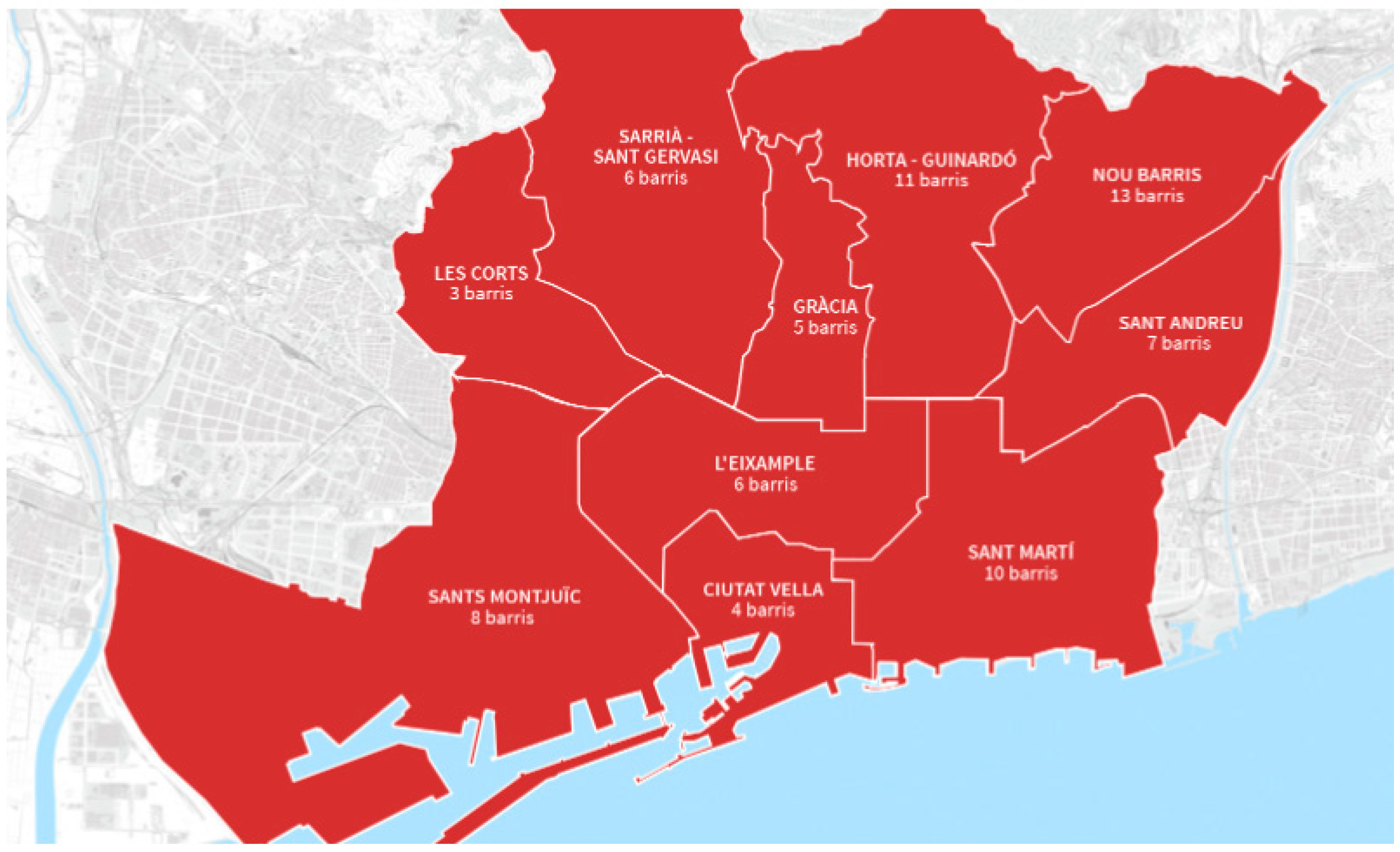
Districts
D1	Ciutat Vella
D2	Eixample
D3	Nou Barris
D4	Gràcia
D5	Horta-Guinardó
D6	Les Corts
D7	Sant Andreu
D8	Sant Martí
D9	Sants-Montjuïc
D10	Sarrià-Sant Gervasi

:

To carry out our study, we structured the 701 valid responses from customers into 10 groups established randomly.

Regarding the characteristics of the establishments, we determined 11 that we have been able to structure into three blocks: External appearance (

Table 3. External appearance.

External Appearance
Cr1	Opening hours
Cr2	Establishment poster
Cr3	Exterior cleaning
Cr4	Exhibition and sale of products outside the establishment

), internal organization (

Table 4. Internal organization.

Internal Organization
Cr5	Comfort
Cr6	Good distribution and organization
Cr7	The cleanliness of the establishment
Cr8	The products are correctly labeled

), and customer service (

Table 5. External Appearance.

Customer Service
Cr9	Cordiality when entering and leaving the store
Cr10	Uniformity of employees
Cr11	The care received

).

On the other hand, we brought together four experts in the retail sector; a fundamental requirement is to have a global vision of the market, focusing on the characteristics of the city of Barcelona. The experts consulted were:

20.

Miquel Àngel de Garro. Pimec Comerç Director, lawyer and planner, specializing in trade and distribution;

21.

Maria Paz Carreira. Skilled in Business Planning, Market Research, Marketing, Marketing Strategy, and Product Management;

22.

Marta Raurell i Molera. Head of the Trade, Crafts and Fashion Area, Business and knowledge Department (Generalitat of Catalonia, Spanish Regional Government);

23.

Pau Fusté i Trepat. Trade Technician of the Trade Support Office. Economic development area at Diputació de Barcelona.

With this information, the group of experts describes the grocery stores according to the characteristics established for each of the city’s districts; in aggregated form, the results are shown in

Table 6. Valuations of experts.

	External Appearance				Internal Organization				Customer Service
	Cr1	Cr2	Cr3	Cr4	Cr5	Cr6	Cr7	Cr8	Cr9	Cr10	Cr11
D1	0.538	0.538	0.700	0.588	0.718	0.675	0.725	0.775	0.688	0.338	0.755
D2	0.700	0.738	0.863	0.573	0.848	0.828	0.863	0.750	0.823	0.663	0.848
D3	0.675	0.650	0.813	0.563	0.738	0.710	0.820	0.655	0.795	0.560	0.823
D4	0.700	0.775	0.760	0.623	0.738	0.718	0.800	0.785	0.800	0.525	0.848
D5	0.675	0.750	0.780	0.595	0.723	0.708	0.800	0.683	0.820	0.525	0.845
D6	0.700	0.738	0.870	0.598	0.850	0.855	0.888	0.738	0.850	0.600	0.875
D7	0.700	0.743	0.838	0.598	0.870	0.818	0.850	0.775	0.825	0.585	0.848
D8	0.688	0.698	0.775	0.563	0.733	0.723	0.805	0.738	0.800	0.550	0.808
D9	0.675	0.750	0.773	0.625	0.730	0.690	0.830	0.775	0.775	0.538	0.848
D10	0.700	0.800	0.888	0.615	0.900	0.855	0.923	0.795	0.870	0.700	0.913

.

We assumed that each group of consumers has similar characteristics, so we can determine their evaluations of each of the characteristics of the establishments, and their aggregate subjective opinions are shown in

Table 7. Valuations of consumers.

	External Appearance				Internal Organization				Customer Service
	Cr1	Cr2	Cr3	Cr4	Cr5	Cr6	Cr7	Cr8	Cr9	Cr10	Cr11
Group1	0.500	0.950	0.950	0.500	0.800	0.700	0.770	0.850	0.880	0.490	0.630
Group2	0.450	0.950	0.860	0.770	0.770	0.770	0.740	0.880	0.850	0.480	0.660
Group3	0.550	0.850	0.870	0.670	0.770	0.720	0.720	0.810	0.770	0.460	0.650
Group4	0.450	0.970	0.940	0.600	0.840	0.790	0.690	0.980	0.800	0.500	0.550
Group5	0.500	0.920	0.840	0.720	0.720	0.700	0.680	0.910	0.770	0.500	0.680
Group6	0.250	0.970	0.860	0.600	0.810	0.780	0.780	0.850	0.820	0.480	0.680
Group7	0.550	0.830	0.890	0.730	0.740	0.760	0.680	0.790	0.800	0.500	0.620
Group8	0.350	0.950	0.760	0.670	0.720	0.720	0.680	0.790	0.800	0.520	0.620
Group9	0.450	0.900	0.850	0.550	0.770	0.750	0.730	0.770	0.810	0.500	0.660
Group10	0.600	0.930	1.000	0.530	0.770	0.760	0.710	0.920	0.850	0.500	0.680

. The results are valuations (numbers) between 0 and 1; 1 being the best result and 0 the worst result.

Now we wanted to observe possible differences in the results obtained with the application of the different concepts that we have developed in Section 2. First, we consider the three types of distances (Hamming, Euclidean, and Minkowski), and the aggregated results are shown in

Table 8. Aggregated distances with Hamming.

	D1	D2	D3	D4	D5	D6	D7	D8	D9	D10
Group1	0.135	0.126	0.122	0.109	0.112	0.128	0.121	0.112	0.115	0.136
Group2	0.137	0.132	0.134	0.109	0.119	0.130	0.121	0.122	0.118	0.142
Group3	0.093	0.110	0.099	0.074	0.088	0.112	0.100	0.088	0.078	0.123
Group4	0.157	0.138	0.153	0.132	0.142	0.140	0.128	0.141	0.141	0.151
Group5	0.111	0.139	0.116	0.093	0.103	0.143	0.126	0.107	0.093	0.154
Group6	0.143	0.121	0.132	0.111	0.117	0.125	0.111	0.120	0.120	0.139
Group7	0.110	0.113	0.104	0.079	0.093	0.115	0.103	0.092	0.088	0.124
Group8	0.116	0.147	0.121	0.086	0.101	0.150	0.133	0.102	0.096	0.163
Group9	0.105	0.102	0.095	0.083	0.087	0.110	0.095	0.083	0.090	0.129
Group10	0.137	0.118	0.117	0.103	0.108	0.120	0.113	0.105	0.112	0.131

,

Table 9. Aggregated distances with Euclidean.

	D1	D2	D3	D4	D5	D6	D7	D8	D9	D10
Group1	0.174	0.140	0.147	0.130	0.133	0.144	0.133	0.133	0.132	0.155
Group2	0.169	0.153	0.161	0.128	0.139	0.152	0.141	0.144	0.132	0.162
Group3	0.125	0.124	0.115	0.093	0.100	0.126	0.111	0.100	0.094	0.148
Group4	0.192	0.171	0.188	0.162	0.174	0.176	0.162	0.170	0.166	0.183
Group5	0.149	0.149	0.147	0.112	0.126	0.153	0.138	0.128	0.114	0.165
Group6	0.183	0.176	0.182	0.164	0.167	0.176	0.168	0.170	0.163	0.184
Group7	0.138	0.130	0.123	0.106	0.110	0.133	0.120	0.111	0.108	0.154
Group8	0.161	0.171	0.163	0.142	0.144	0.176	0.164	0.149	0.143	0.190
Group9	0.142	0.128	0.124	0.111	0.109	0.132	0.121	0.111	0.112	0.151
Group10	0.176	0.130	0.146	0.121	0.131	0.134	0.123	0.128	0.126	0.144

and

Table 10. Aggregated distances with Minkowski.

	D1	D2	D3	D4	D5	D6	D7	D8	D9	D10
Group1	0.209	0.151	0.167	0.145	0.146	0.156	0.145	0.149	0.145	0.169
Group2	0.202	0.166	0.180	0.145	0.154	0.165	0.155	0.161	0.144	0.175
Group3	0.154	0.134	0.127	0.108	0.110	0.136	0.120	0.108	0.107	0.165
Group4	0.223	0.191	0.212	0.181	0.195	0.199	0.184	0.188	0.182	0.206
Group5	0.184	0.155	0.167	0.124	0.141	0.160	0.145	0.141	0.126	0.174
Group6	0.220	0.219	0.223	0.212	0.207	0.219	0.215	0.215	0.205	0.224
Group7	0.158	0.143	0.135	0.123	0.124	0.148	0.134	0.122	0.124	0.174
Group8	0.200	0.193	0.191	0.178	0.173	0.198	0.189	0.180	0.174	0.210
Group9	0.175	0.146	0.146	0.133	0.127	0.149	0.140	0.133	0.129	0.168
Group10	0.209	0.138	0.168	0.136	0.149	0.143	0.131	0.146	0.139	0.154

.

Second, we develop the application of the OWA operators. In the case of the OWAD operator, the experts determined the associated weighting vectors; W = (0.010, 0.100, 0.050, 0.050, 0.080, 0.150, 0.250, 0.200, 0.050, and 0.060) and the order of inducing variables was U = (8.6, 6.4, 6.8, 5.7, 6.2, 7.3, 5.1, 7.6, 5.4, and 3.2) in the IOWAD operator and the aggregated results that we obtained, are shown in

Table 11. Aggregated distances with the OWAD operator.

	D1	D2	D3	D4	D5	D6	D7	D8	D9	D10
Group1	0.109	0.115	0.100	0.094	0.102	0.121	0.110	0.094	0.103	0.131
Group2	0.115	0.127	0.109	0.090	0.100	0.128	0.116	0.104	0.106	0.138
Group3	0.075	0.107	0.096	0.063	0.082	0.104	0.097	0.089	0.067	0.114
Group4	0.137	0.119	0.136	0.121	0.131	0.116	0.107	0.127	0.132	0.126
Group5	0.087	0.146	0.100	0.085	0.091	0.144	0.130	0.095	0.085	0.147
Group6	0.119	0.087	0.101	0.080	0.090	0.097	0.081	0.094	0.093	0.106
Group7	0.097	0.105	0.099	0.063	0.086	0.109	0.094	0.085	0.077	0.114
Group8	0.087	0.131	0.100	0.050	0.071	0.131	0.110	0.072	0.063	0.156
Group9	0.086	0.085	0.075	0.065	0.073	0.097	0.084	0.065	0.077	0.116
Group10	0.111	0.114	0.096	0.092	0.091	0.115	0.108	0.088	0.099	0.126

and

Table 12. Aggregated distances with the IOWAD operator.

	D1	D2	D3	D4	D5	D6	D7	D8	D9	D10
Group1	0.138	0.093	0.106	0.100	0.102	0.098	0.098	0.095	0.110	0.099
Group2	0.151	0.119	0.134	0.097	0.113	0.112	0.111	0.122	0.108	0.115
Group3	0.091	0.088	0.087	0.052	0.076	0.091	0.081	0.077	0.052	0.093
Group4	0.131	0.086	0.115	0.089	0.102	0.089	0.079	0.103	0.101	0.097
Group5	0.111	0.126	0.112	0.077	0.096	0.129	0.117	0.101	0.074	0.132
Group6	0.110	0.063	0.090	0.064	0.069	0.067	0.056	0.077	0.076	0.077
Group7	0.111	0.099	0.095	0.058	0.082	0.102	0.092	0.083	0.069	0.104
Group8	0.096	0.104	0.090	0.048	0.070	0.108	0.095	0.073	0.058	0.111
Group9	0.091	0.059	0.061	0.057	0.060	0.075	0.065	0.048	0.067	0.092
Group10	0.128	0.089	0.098	0.091	0.094	0.093	0.094	0.085	0.103	0.103

.

From the aggregated distances, we proceeded to calculate the Branch-and-bound algorithm using the three types of distances, the OWAD operator and the IOWAD operator.

The results of the assignment process in which we have used the concept of distance are shown in

Table 13. Assignation process.

ORDER	HAMMING		EUCLIDEAN		MINKOWSKI
1	Group8	D4	Group5	D4	Group6	D1
2	Group4	D10	Group2	D9	Group7	D3
3	Group6	D7	Group8	D1	Group3	D8
4	Group10	D2	Group9	D5	Group5	D4
5	Group2	D6	Group7	D3	Group2	D9
6	Group9	D8	Group3	D8	Group8	D5
7	Group3	D1	Group4	D7	Group1	D2
8	Group5	D9	Group6	D10	Group9	D6
9	Group1	D3	Group10	D2	Group10	D7
10	Group7	D5	Group1	D6	Group4	D10

.

The results show us that D₄ (Gràcia) in order 1 and D₈ (Sant Martí) in order 6 coincide in their positions in the process of assigning the Hamming and Euclidean distances. There are no coincidences with the results obtained in the assignment process from the Minkowski distance. However, if we compare the consumer groups, the allocation results coincide in the cases of Hamming and Minkowski only for Group 2 in order 5, and in Euclidean and Minkowski for Group 10 in order 9.

Next, we developed the Branch-and-bound algorithm with the OWAD operator. We assumed that $W=\left(0.010,0.100,0.050,0.050,0.080,0.150,0.250,0.200,0.050,\mathrm{and}0.060\right)$. The results are shown in

Table 14. Assignation process with OWAD operator.

ORDER	OWAD
1	Group7	D4
2	Group4	D6
3	Group6	D7
4	Group5	D1
5	Group3	D9
6	Group2	D5
7	Group8	D8
8	Group9	D2
9	Group10	D10
10	Group1	D3

.

In this case, we can see that the first assignment corresponds to Group 7 with D₄ (Gràcia). We observed that D₄ is assigned in order 1 as when we have used the Hamming and Euclidean distances, although with different groups of consumers. Group 4 was then assigned to D₆ (Les Corts). Regarding the last assignments, we found that Group 10 was assigned to D₁₀ (Sarriá—Sant Gervasi), and Group 1, in last place, was assigned to D₃ (Nou Barris). In view of the data, no relationship was observed between income level and consumer preferences.

Next, we developed a Hungarian algorithm with the IOWAD operator. We assumed that $U=\left(8.6,6.4,6.8,5.7,6.2,7.3,5.1,7.6,5.4,\mathrm{and}3.2\right)$. The results are shown in

Table 15. Assignation process with IOWAD operator.

ORDER	IOWAD
1	Group1	D10
2	Group7	D4
3	Group8	D9
4	Group3	D1
5	Group5	D5
6	Group2	D6
7	Group10	D2
8	Group4	D7
9	Group6	D8
10	Group9	D3

.

With the use of the IOWAD operator, we can see that D₄ (Gràcia) was assigned in order 2 to Group 7 as we have determined with the OWAD operator but in order 1. In this assignment process, first Group 1 was assigned to D₁₀ (Sarrià—Sant Gervasi), which is the District of Barcelona with the highest per capita income [59]. This relationship between the order of assignment and the income level of the districts was not fulfilled in the rest.

4. Conclusions

In this paper, based on the contribution made by Jaime Gil-Aluja [51], we have developed a new extension of the Fuzzy Branch-and-bound algorithm for decision-making with the use of the OWA operators.

The algorithm that we develop is analogous to the original idea, but its complexity is given by the fact that the decision-maker can consider optimistic or pessimistic scenarios by underestimating or overestimating the information available to them. To give our approach more projection, we have developed it by using induced aggregation operators. As a result, we have been able to analyze environments or situations where the information provided is not entirely clear.

The applicability of this new approach has been analyzed in the case of consumer decision-making in the city of Barcelona, where we have developed an illustrative example where, thanks to the application of the different algorithms, we have determined for each case the district of the city that best adapts to the characteristics of consumers. In this approach, we considered complex environments where the opinion of various consumer experts has been necessary. We were able to observe that with the application of each one of the aggregation operators, we obtained different assignments. With the application of the OWAD and IOWAD operators, we can consider depending on the situation in which we find ourselves different degrees of optimism or pessimism in the analysis.

The main contribution of our research focuses on the fact that we can consider the information in a broader way, thanks to the use of aggregation operators that allow us to contemplate from the minimum distance to the maximum. In our future research, we hope to develop more extensions by adding new types of aggregation operators. We will also consider carrying out other decision-making applications such as product management, new market management, and strategic company management.

References

- Salesforce Homepage. Available online: https://www.salesforce.com/news/stories/q1-shopping-index-global-digital-commerce-grew-58-percent-stimulus-checks-boost-u-s-sales/ (accessed on 20 September 2021).
- Bellini, S.; Cardinali, M.G.; Grandi, B. A structural equation model of impulse buying behavior in grocery retailing. J. Retail. Consum. Serv. 2017, 36, 164–171. [Google Scholar] [CrossRef]
- Volpe, R.; Jaenicke, E.C.; Chenarides, L. Store formats, markets structure and consumers food shopping decisions. Appl. Econ. Perspect. Policy 2018, 40, 672–694. [Google Scholar] [CrossRef]
- Printezis, I.; Grebitus, C. Marketing channels for local food. Ecol. Econ. 2018, 152, 161–171. [Google Scholar] [CrossRef]
- Achon, M.; Serrano, M.; Garcia-Gonzalez, A.; Alonso-Aperte, E.; Varela-Moreiras, G. Present food shopping habits in the Spanish adult population: A cross-sectional study. Nutrients 2017, 9, 508. [Google Scholar] [CrossRef] [PubMed]
- Hoek, A.C. Healthy and environmentally sustainable food choices: Consumer responses to point-of-purchase actions. Food Qual. Prefer. 2017, 58, 94–106. [Google Scholar] [CrossRef]
- Stranieri, S.; Ricci, E.C.; Banterle, A. Convenience food with environmentally-sustainable attributes: A consumer perspective. Appetite 2017, 116, 11–20. [Google Scholar] [CrossRef]
- Gil-Aluja, J. Elements for a Theory of Decision in Uncertainty; Kluwer Academic Publishers: Dordrecht, The Netherlands, 1999. [Google Scholar]
- Merigó, J.M.; Palacios-Marqués, D.; Soto-Acosta, P. Distance measures, weighted averages, OWA operators and Bonferroni means. Appl. Soft Comput. 2017, 50, 356–366. [Google Scholar] [CrossRef]
- Zhou, F.; Chen, T.Y. Multiple criteria group decision analysis using a Pythagorean fuzzy programming model for multidimensional analysis of preference based on novel distance measures. Comput. Ind. Eng. 2020, 148, 106670. [Google Scholar] [CrossRef]
- Dai, S.; Pei, D.; Wang, S.M. Perturbation of fuzzy sets and fuzzy reasoning based on normalized Minkowski distances. Fuzzy Sets Syst. 2012, 189, 63–73. [Google Scholar] [CrossRef]
- Linares-Mustarós, S.; Ferrer-Comalat, J.C.; Corominas-Coll, D.; Merigó, J.M. The weighted average multiexperton. Inf. Sci. 2021, 557, 355–372. [Google Scholar] [CrossRef]
- Dubois, D. Fuzzy weighted averages and fuzzy convex sums: Author’s response. Fuzzy Sets Syst. 2013, 213, 106–108. [Google Scholar] [CrossRef] [Green Version]
- Yager, R.R. On ordered weighted averaging aggregation operators in multi-criteria decision making. IEEE Trans. Syst. Man Cybern. 1988, 18, 183–190. [Google Scholar] [CrossRef]
- Torra, V. Andness directedness for operators of the OWA and WOWA families. Fuzzy Sets Syst. 2021, 414, 28–37. [Google Scholar] [CrossRef]
- Nguyen, J.; Armisen, A.; Sánchez-Hernández, G.; Casabayó, M.; Agell, N. An OWA-based hierarchical clustering approach to understanding users’ lifestyles. Knowl.-Based Syst. 2020, 190, 105308. [Google Scholar] [CrossRef]
- Bueno, I.; Carrasco, R.A.; Ureña, R.; Herrera-Viedma, E. Application of an opinion consensus aggregation model based on OWA operators to the recommendation of tourist sites. Procedia Comput. Sci. 2019, 162, 539–546. [Google Scholar] [CrossRef]
- Reimann, O.; Schumacher, C.; Vetschera, R. How well does the OWA operator represent real preferences? Eur. J. Oper. Res. 2017, 258, 993–1003. [Google Scholar] [CrossRef]
- De Miguel, L.; Sesma-Sara, M.; Elkano, M.; Asiain, M.; Bustince, H. An algorithm for group decision making using n-dimensional fuzzy sets, admissible orders and OWA operators. Inf. Fusion 2017, 37, 126–131. [Google Scholar] [CrossRef] [Green Version]
- Flores-Sosa, M.; Avilés-Ochoa, E.; Merigó, J.M.; Yager, R.R. Volatility GARCH models with the ordered weighted average (OWA) operators. Inf. Sci. 2021, 565, 46–61. [Google Scholar] [CrossRef]
- Liu, F.; Liu, Z.L.; Wu, Y.H. A group decision making model based on triangular fuzzy additive reciprocal matrices with additive approximation-consistency. Appl. Soft Comput. 2018, 65, 349–359. [Google Scholar] [CrossRef]
- Zeng, S.; Hu, Y.; Xie, X. Q-rung orthopair fuzzy weighted induced logarithmic distance measures and their application in multiple attribute decision making. Eng. Appl. Artif. Intell. 2021, 100, 104167. [Google Scholar] [CrossRef]
- Zhang, C.; Hu, Q.; Zeng, S.; Su, W. IOWLAD-based MCDM model for the site assessment of a household waste processing plant under a Pythagorean fuzzy environment. Environ. Impact Assess. Rev. 2021, 89, 106579. [Google Scholar] [CrossRef]
- Jin, L.; Kalina, M.; Qian, G. Discrete and continuous recursive forms of OWA operators. Fuzzy Sets Syst. 2017, 308, 106–122. [Google Scholar] [CrossRef]
- Flores-Sosa, M.; Aviles-Ochoa, E.; Merigo, J.M. Induced OWA operators in linear regression. J. Intell. Fuzzy Syst. 2020, 38, 5509–5520. [Google Scholar] [CrossRef]
- León-Castro, E.; Espinoza-Audelo, L.F.; Merigó, J.M.; Herrera-Viedma, E.; Herrera, F. Measuring volatility based on ordered weighted average operators: The case of agricultural product prices. Fuzzy Sets Syst. 2021, 422, 161–176. [Google Scholar] [CrossRef]
- Zheng, X.; Deng, Y. Dependence assessment in human reliability analysis based on evidence credibility decay model and IOWA operator. Ann. Nucl. Energy 2018, 112, 673–684. [Google Scholar] [CrossRef]
- Land, A.H.; Doig, A.G. An Automatic Method of Solving Discrete Programming Problems. Econometrica 1960, 28, 497–520. [Google Scholar] [CrossRef]
- Little, J.D.C.; Murty, K.G.; Sweeney, D.W.; Karel, C. An algorithm for the traveling salesman problem. Oper. Res. 1963, 11, 972–989. [Google Scholar] [CrossRef] [Green Version]
- Kim, D.G. A branch and bound algorithm for determining locations of long-term care facilities. Eur. J. Oper. Res. 2010, 206, 168–177. [Google Scholar] [CrossRef]
- Qin, H.; Zhang, Z.Z.; Liang, X.C. An enhanced branch-and-bound algorithm for the talent scheduling problem. Eur. J. Oper. Res. 2016, 250, 412–426. [Google Scholar] [CrossRef] [Green Version]
- Sölveling, G.; Clarke, J.P. Scheduling of airport runway operations using stochastic branch and bound methods. Transp. Res. C Emerg. Technol. 2014, 45, 119–137. [Google Scholar] [CrossRef]
- Ho, T.Y.; Liu, S.; Zabinsky, Z.B. A branch and bound algorithm for dynamic resource allocation in population disease management. Oper. Res. Lett. 2019, 47, 579–586. [Google Scholar] [CrossRef]
- Madakat, D.; Morio, J.; Vanderpooten, D. A biobjective branch and bound procedure for planning spatial missions. Aerosp. Sci. Technol. 2018, 73, 269–277. [Google Scholar] [CrossRef] [Green Version]
- Hao, Z.; Xu, Z.; Zhao, H.; Zhang, R. The context-based distance measure for intuitionistic fuzzy set with application in marine energy transportation route decision making. Appl. Soft Comput. 2021, 101, 107044. [Google Scholar] [CrossRef]
- Ramos-Guajardo, A.B.; Ferraro, M.B. A fuzzy clustering approach for fuzzy data based on a generalized distance. Fuzzy Sets Syst. 2020, 389, 29–50. [Google Scholar] [CrossRef] [Green Version]
- Hu, M.; Lan, J.; Wang, Z. A distance measure, similarity measure and possibility degree for hesitant interval-valued fuzzy sets. Comput. Ind. Eng. 2019, 137, 106088. [Google Scholar] [CrossRef]
- Vigier, H.P.; Scherger, V.; Terceño, A. An application of OWA operators in fuzzy business diagnosis. Appl. Soft Comput. 2017, 54, 440–448. [Google Scholar] [CrossRef]
- Kacprzyk, J.; Yager, R.R.; Merigó, J.M. Towards human-centric aggregation via ordered weighted aggregation operators and linguistic data summaries: A new perspective on Zadeh’s inspirations. IEEE Comput. Intell. Mag. 2019, 14, 16–30. [Google Scholar] [CrossRef]
- Merigó, J.M.; Gil-Lafuente, A.M.; Yu, D.; Llopis-Albert, C. Fuzzy decision making in complex frameworks with generalized aggregation operators. Appl. Soft Comput. 2018, 68, 314–321. [Google Scholar] [CrossRef]
- Zou, T.; He, F.; Cai, M.; Li, Y. Methods for describing different results obtained from different methods in accident reconstruction. Forensic Sci. Int. 2018, 291, 253–259. [Google Scholar] [CrossRef] [PubMed]
- Liu, H.; Cai, J.; Martínez, L. The importance weighted continuous generalized ordered weighted averaging operator and its application to group decision making. Knowl.-Based Syst. 2013, 48, 24–36. [Google Scholar] [CrossRef]
- Zeng, S.; Merigó, J.M.; Su, W. The uncertain probabilistic OWA distance operator and its application in group decision making. Appl. Math. Model. 2013, 37, 6266–6275. [Google Scholar] [CrossRef]
- Blanco-Mesa, F.; Merigó, J.M.; Kacprzyk, J. Bonferroni means with distance measures and the adequacy coefficient in entrepreneurial group theory. Knowl.-Based Syst. 2016, 111, 217–227. [Google Scholar] [CrossRef]
- Yager, R.R.; Filev, D.P. Induced ordered weighted averaging operators. IEEE Trans. Syst. Man Cybern. B 1999, 29, 141–150. [Google Scholar] [CrossRef] [PubMed]
- Pang, J.; Liu, X.; Huang, Q. A new quality evaluation system of soil and water conservation for sustainable agricultural development. Agric. Water Manag. 2020, 240, 106235. [Google Scholar] [CrossRef]
- Sabbaghian, R.J.; Zarghami, M.; Nejadhashemi, A.P.; Sharifi, M.B.; Herman, M.R.; Daneshvar, F. Application of risk-based multiple criteria decision analysis for selection of the best agricultural scenario for effective watershed management. J. Environ. Manag. 2016, 168, 260–272. [Google Scholar] [CrossRef] [PubMed]
- Merigó, J.M.; Casanovas, M. Decision-making with distance measures and induced aggregation operators. Comput. Ind. Eng. 2011, 60, 66–76. [Google Scholar] [CrossRef] [Green Version]
- Chen, H.Y.; Zhou, L.G. An approach to group decision making with interval fuzzy preference relations based on induced generalized continuous ordered weighted averaging operator. Expert Syst. Appl. 2011, 38, 13432–13440. [Google Scholar] [CrossRef]
- Blanco-Mesa, F.; León-Castro, E.; Merigó, J.M. Bonferroni induced heavy operators in ERM decision-making: A case on large companies in Colombia. Appl. Soft Comput. 2018, 72, 371–391. [Google Scholar] [CrossRef]
- Morrison, D.R.; Jacobson, S.H.; Sauppe, J.J.; Sewell, E.C. Branch-and-bound algorithms: A survey of recent advances in searching, branching, and pruning. Discret. Optim. 2016, 19, 79–102. [Google Scholar] [CrossRef]
- Gil-Aluja, J. The Interactive Management of the Human Resources in Uncertainty; Kluwer Academic Publishers: Dordrecht, The Netherlands, 1998; pp. 170–172. [Google Scholar]
- Hamming, R.W. Error-detecting and error-correcting codes. Bell Syst. Tech. J. 1950, 29, 147–160. [Google Scholar] [CrossRef]
- Szmidt, E.; Kacprzyk, J. Distances between intuitionistic fuzzy sets. Fuzzy Sets Syst. 2000, 114, 505–518. [Google Scholar] [CrossRef]
- Shouzhen, Z. An Extension of OWAD Operator and Its Application to Uncertain Multiple-Attribute Group Decision-Making. Cybern. Syst. 2016, 47, 363–375. [Google Scholar] [CrossRef]
- Vizuete-Luciano, E.; Merigó, J.M.; Boria-Reverter, S.; Gil-Lafuente, A.M. Decision Making in the Assignment Process by Using the Hungarian Algorithm with OWA Operators. Technol. Econ. Dev. Econ. 2015, 21, 684–704. [Google Scholar] [CrossRef]
- Casanovas, M.; Torres-Martinez, A.; Merigó, J.M. Multi-person and multi-criteria decision making with the induced probabilistic ordered weighted average distance. Soft Comput. 2020, 24, 1435–1446. [Google Scholar] [CrossRef]
- Wei, G.W.; Zhao, X.; Wang, H. An approach to multiple attribute group decision making with interval intuitionistic trapezoidal fuzzy information. Technol. Econ. Dev. Econ. 2012, 18, 317–330. [Google Scholar] [CrossRef] [Green Version]
- Ajuntament de Barcelona Homepage. Available online: https://ajuntament.barcelona.cat/estadistica/castella/Estadistiques_per_territori/Barris/Economia/Renda_disponible_llars/T012.htm (accessed on 15 November 2021).