Implicit Solitary Waves for One of the Generalized Nonlinear Schrödinger Equations

Abstract

Application of transformations for dependent and independent variables is used for finding solitary wave solutions of the generalized Schrödinger equations. This new form of equation can be considered as the model for the description of propagation pulse in a nonlinear optics. The method for finding solutions of equation is given in the general case. Solitary waves of equation are obtained as implicit function taking into account the transformation of variables.

1. Introduction

In this paper, we consider the nonlinear partial differential equation

$$\begin{array}{c}i{q}_t+q_{xx}+\alpha q+{\beta \left|q\right|}^{n}q+{\gamma \left|q\right|}^{2n}q+{\delta \left|q\right|}^{3n}q+\lambda {\left|q\right|}^{4n}q=0,\end{array}$$

(1)

where $q(x,t)$ is complex function, x is coordinate, t is time, n is rational number and $\alpha$, $\beta$, $\gamma$, $\delta$, $\lambda$ are parameters of Equation (1). It is easy to see that Equation (1) is the generalization of the famous nonlinear Schrödinger equation which follows from Equation (1) at $\beta \ne 0$, $n=2$, $\alpha =\gamma =\delta =\lambda =0$. Equation (1) has been presented in recent paper [1] as an equation whose solution can be obtained using the method of transformation for dependent and independent variables. Equation (1) is the generalization of some equations describing propagation pulses in the nonlinear optics (see, for example, [2,3,4,5,6,7,8,9,10,11,12,13,14,15,16,17,18,19]).

The purpose of this paper is to present the method for finding solutions of Equation (1) and to obtain the implicit solitary wave solutions of Equation (1) using the transformations of variables.

This article is organized as follows. In Section 2, the method of finding solutions of Equation (1) is presented taking into account the traveling wave reduction. In this Section the general approach to finding exact solutions of Equation (1) is described as weel. The implicit solitary waves of Equation (1) in form of kink are given in Section 3. Implicit soliton solutions of Equation (1) are presented in Section 4.

2. Method Applied

Let us look for the exact solution of Equation (1) using the the form

$$\begin{array}{c}q(x,t)=y\left(z\right)e^{i(kx-\omega t)},\end{array}$$

(2)

where $y\left(z\right)$ is a function describing an optical pulse profile, $\omega$ is a frequency and k is a wave number and z is a variable of x and t: $z=x-C_{0}t$.

Substituting (2) into Equation (1) and equating expressions for real and imaginary parts yields the overdetermined system of equations for function $y\left(z\right)$ in the form

$$\begin{array}{c}(2k-C_0)y_z=0,\end{array}$$

(3)

$$\begin{array}{c}{y}_{zz}+(\omega -k^2)y+\alpha y+\beta y^{n+1}-\gamma y^{2n+1}-\delta y^{3n+1}+\lambda y^{4n+1}=0.\end{array}$$

(4)

Provided that $C_0=2k$ we see that Equation (3) is satisfied. Multiplying Equation (4) by $y_z$ and integrating over z, we obtain the first integral in the form

$$\begin{gathered} \begin{array}{c}{y}_z^2+(\omega +\alpha -k^2)y^2+\frac{2\beta }{n+2}{y}^{n+2}-\frac{\gamma }{n+1}{y}^{2n+2}-\end{array} \\ \frac{2\delta }{3n+2}{y}^{3n+2}+\frac{\lambda }{2n+1}{y}^{4n+2}=C_1, \end{gathered}$$

(5)

where $C_1$ is a constant of integration.

Solution of Equation (5) can be written in the form of quadrature

$$\begin{array}{c}\int \frac{d\xi }{\sqrt{H\left[y\right]}}=z-z_0,\end{array}$$

(6)

where

$$\begin{gathered} \begin{array}{c}H\left[y\right]=C_1-(\omega +\alpha -k^2)y^2-\frac{2\beta }{n+2}{y}^{n+2}+\frac{\gamma }{n+1}{y}^{2n+2}+\end{array} \\ \frac{2\delta }{3n+2}{y}^{3n+2}-\frac{\lambda }{2n+1}{y}^{4n+2}. \end{gathered}$$

(7)

However integral (6) cannot be calculated in the general case.

Let us look for solution of Equation (5) in the form

$$\begin{array}{c}y\left(z\right)=F\left(\xi \right),{\xi }_z=F{\left(\xi \right)}^n.\end{array}$$

(8)

Using (8), we have

$$\begin{array}{c}{y}_z=F_{\xi }{\xi }_z=F_{\xi }F{\left(\xi \right)}^n.\end{array}$$

(9)

Substituting (8) and (9) into Equation (5), we obtain the equation

$$\begin{array}{c}{F}_{\xi }^2+(\omega +\alpha -k^2)F^{2-2n}+\frac{2\beta }{n+2}{F}^{2-n}-\frac{\gamma }{n+1}{F}^2-\\ \frac{2\delta }{3n+2}{F}^{n+2}+\frac{\lambda }{2n+1}{F}^{2n+2}=0.\end{array}$$

(10)

Equation (10) has been previously studied in papers [1,2,3]. It is important to note that by using the transformation [20,21,22,23]

$$\begin{array}{c}F\left(\xi \right)=V{\left(\xi \right)}^{-\frac{1}{n}},\end{array}$$

(11)

Equation (10) can be reduced to the equation with solutions in the form of elliptic function

$$\begin{array}{c}{V}_{\xi }^2+(\omega +\alpha -k^2)n^2{V}^4+\frac{2n^2\beta }{n+2}{V}^3-\frac{n^2\gamma }{n+1}{V}^2-\\ \\ \frac{2n^2\delta }{3n+2}V+\frac{n^2\lambda }{2n+1}=0.\end{array}$$

(12)

Solution of Equation (12) can be searched for in the form [24,25,26]

$$\begin{array}{c}V\left(\xi \right)=V_1+\frac{(V_2-V_1)E}{Y^2+E},E=\frac{(V_1-V_3)}{(V_3-V_2)},\end{array}$$

(13)

where $V_1$, $V_2$, $V_3$ and $V_4$ are the roots of the following algebraic equation

$$\begin{array}{c}(\omega +\alpha -k^2)V^4+\frac{2\beta }{n+2}{V}^3-\frac{\gamma }{n+1}{V}^2-\frac{2\delta }{3n+2}V+\frac{\lambda }{2n+1}=0\end{array}$$

(14)

and $Y\left(\xi \right)$ is the Jacobi elliptic sine in the form

$$\begin{array}{c}Y(\xi ;k)=\mathrm{sn}\left\{\frac{n}{2}\sqrt{a(V_4-V_2)(V_1-V_3)}(\xi -{\xi }_0);S\right\},\end{array}$$

(15)

where S is determined by the formula

$$S^2=\frac{(V_1-V_4)(V_1-V_3)}{(V_4-V_2)(V_3-V_2)}.$$

(16)

Taking into account (11), the solution $F\left(\xi \right)$ can be expressed by the formula

$$\begin{array}{c}F\left(\xi \right)={\left[\frac{V_1(V_3-V_2){\mathrm{sn}}^2\left\{\frac{n}{2}\sqrt{a(V_4-V_2)(V_1-V_3)}(\xi -{\xi }_0);S\right\}+V_2(V_1-V_3)}{(V_3-V_2){\mathrm{sn}}^2\left\{\frac{1}{2}\sqrt{d(V_4-V_2)(V_1-V_3)}(\xi -{\xi }_0);S\right\}+V_1-V_3}\right]}^{-\frac{1}{n}}.\end{array}$$

(17)

We cannot find the explicit expression for the function $\xi \left(z\right)$ using $V\left(\xi \right)$ in the general case by means of the formula

$$\begin{array}{c}\int V\left(\xi \right)d\xi =z-z_0.\end{array}$$

(18)

However in the case of solitary wave solutions these solutions of Equation (1) can be found as the implicit functions. To look for these solutions we use the special methods has been developing in the last few years [27,28,29,30,31,32,33,34,35,36].

3. Implicit Solitary Wave Solutions of the Generalized Nonlinear Schrödinger Equation in Form Kink

Let us look for the solution of Equation (12) using the logistic function. We assume that there exist a solution of Equation (12) in the form [37,38,39,40,41,42,43,44,45,46]

$$\begin{array}{c}V\left(\xi \right)=A_0+A_{1}Q\left(\xi \right),\end{array}$$

(19)

where $Q\left(\xi \right)$ is the logistic function [37]

$$\begin{array}{c}Q\left(\xi \right)=\frac{1}{1+{\mathrm{e}}^{m(\xi -{\xi }_0)}}.\end{array}$$

(20)

The function $Q\left(\xi \right)$ is the solution of the Riccati equation in the form

$$\begin{array}{c}{Q}_{\xi }=m(Q^2-Q).\end{array}$$

(21)

The function $Q\left(\xi \right)$ satisfies the following second-order differential equation as well

$$\begin{array}{c}{Q}_{\xi \xi }=m^{2}Q(Q-1)(2Q-1).\end{array}$$

(22)

Substituting (19) into Equation (12) and taking Equations (21) and (22) into account, yields the equality

$$\begin{array}{c}\left(n^2{A_1}^4\omega -n^2{A_1}^4{k}^2+n^2{A_1}^4\alpha +{A_1}^2{m}^2\right)Q^4+\left(4n^2{A}_0{A_1}^3\alpha -\right.\\ \left.2{A_1}^2{m}^2-4n^2{A}_0{A_1}^3{k}^2+4n^2{A}_0{A_1}^3\omega +\frac{2n^2{A_1}^3\beta }{2+n}\right)Q^3+\left({A_1}^2{m}^2+\right.\\ \frac{6n^2{A}_0{A_1}^2\beta }{2+n}+6n^2{A_0}^2{A_1}^2\alpha +6n^2{A_0}^2{A_1}^2\omega -\frac{n^2{A_1}^{2}g}{1+n}-\\ \left.6n^2{A_0}^2{A_1}^2{k}^2\right)Q^2+\left(\frac{6n^2{A_0}^2{A}_1\beta }{2+n}-\frac{2n^2{A}_0{A}_{1}g}{1+n}-\frac{2n^2{A}_1\delta }{2+3n}-\right.\\ \left.4n^2{A_0}^3{A}_1{k}^2+4n^2{A_0}^3{A}_1\alpha +4n^2{A_0}^3{A}_1\omega \right)Q-n^2{\mathit{A}\mathit{0}}^4{k}^2+n^2{\mathit{A}\mathit{0}}^4\alpha +\\ n^2{A_0}^4\omega +\frac{\lambda n^2}{1+2n}-2\frac{n^2{A}_0\delta }{2+3n}-\frac{n^2{A_0}^{2}g}{1+n}+2\frac{n^2{A_0}^3\beta }{2+n}=0.\end{array}$$

(23)

We have obtained that a polynomial in solutions $Q\left(z\right)$ is equal to zero. Such thing is possible if and only if all coefficients are equal to zero. Taking into account this property in (23), we derive the conditions for the parameters of Equation (1). These conditions are the following

$$\begin{array}{c}\alpha =k^2-\omega -\frac{m^2}{n^2{A_1}^2},\end{array}$$

(24)

$$\begin{array}{c}\beta =\frac{m^2\left(2+n\right)\left(A_1+2A_0\right)}{n^2{A_1}^2},\end{array}$$

(25)

$$\begin{array}{c}\gamma =\frac{\left(6{A_0}^2+6A_0{A}_1+{A_1}^2\right)m^2\left(1+n\right)}{n^2{A_1}^2},\end{array}$$

(26)

$$\begin{array}{c}\delta =-\frac{\left(2+3n\right)m^2{A}_0\left(2{A_0}^2+3A_0{A}_1+{A_1}^2\right)}{n^2{A_1}^2},\end{array}$$

(27)

$$\begin{array}{c}\lambda =-\frac{\left(1+2n\right)m^2{A_0}^2\left({A_0}^2+2A_0{A}_1+{A_1}^2\right)}{n^2{A_1}^2}.\end{array}$$

(28)

Using solution (19) and definition (18), we get the implicit function $\xi \left(z\right)$ in the form

$$\begin{array}{c}(A_0+A_1)\xi -\frac{A_1}{m}log\left(1+{\mathrm{e}}^{m\xi }\right)=z-z_0.\end{array}$$

(29)

On the other hand taking into account (8) and (11), we obtain

$$\begin{array}{c}\xi =\frac{1}{m}log\left[\frac{(A_0+A_1)y^n-1}{A_0{y}^n-1}\right].\end{array}$$

(30)

Substituting (30) into (29)yields an implicit expression for $y\left(z\right)$ in the form

$$\begin{array}{c}\frac{(A_0+A_1)}{m}log\left[\frac{(A_0+A_1)y^n-1}{A_0{y}^n-1}\right]-\frac{A_1}{m}log\left(\frac{A_1{y}^n}{A_0{y}^n-1}\right)=z-z_0.\end{array}$$

(31)

We have obtained implicit expressions for kinks $y\left(\xi \right)$ and $y\left(z\right)$, where $A_0$, $A_1$, m and n are arbitrary. These values allow us to calculate the parameters $\alpha$, $\beta$, $\gamma$, $\delta$ and $\lambda$ for Equation (5) using conditions (24)–(28).

Solutions (30) of Equation (10) (on the left) and (31) of (5) (on the right) are demonstrated in Figure 1 at $A_0=1.0$, $A_0=0.5$, $n=2$, $m=0.02$ and $z_0=0.0$.

4. Implicit Optical Solitons of the Generalized Nonlinear Schrödinger Equation

Let us obtain the exact solutions in the form of solitons. We look for the solution of Equation (12) in the form [47,48,49,50,51]

$$\begin{array}{c}V\left(\xi \right)=A_0+A_{1}R\left(\xi \right),\end{array}$$

(32)

where the function $R\left(\xi \right)$ solves the following equations

$$\begin{array}{c}{R}_{\xi }^2+a{R}^4+b{R}^3-c{R}^2=0\end{array}$$

(33)

and

$$\begin{array}{c}{R}_{\xi \xi }+2a{R}^3+\frac{3b}{2}{R}^2-cR=0\end{array}$$

(34)

Solution of Equation (33) is as follows [47]

$$\begin{array}{c}R\left(\xi \right)=\frac{4c{\mathrm{e}}^{-\xi \sqrt{c}}}{4ac+b^2+2b{\mathrm{e}}^{-\xi \sqrt{c}}+{\mathrm{e}}^{-2\xi \sqrt{c}}}.\end{array}$$

(35)

Substituting expression (32) and taking into account (33) and (34) into Equation (12), we obtain the following polynomial

$$\begin{array}{c}\left(n^2{A_1}^4\alpha -n^2{A_1}^4{k}^2+n^2{A_1}^4\omega -{A_1}^{2}a\right)R^4+\left(4n^2{A}_0{A_1}^3\alpha -\right.\\ \left.{A_1}^{2}b-4n^2{A}_0{A_1}^3{k}^2+4n^2{A}_0{A_1}^3\omega +\frac{2n^2{A_1}^3\beta }{2+n}\right)R^3+\left({A_1}^{2}c+\right.\\ \frac{6n^2{A}_0{A_1}^2\beta }{2+n}-6n^2{A_0}^2{A_1}^2{k}^2+6n^2{A_0}^2{A_1}^2\alpha +6n^2{A_0}^2{A_1}^2\omega -\\ \left.\frac{n^2{A_1}^{2}g}{1+n}\right)R^2+\left(-2\frac{n^2{A}_0{A}_{1}g}{1+n}+6\frac{n^2{A_0}^2{A}_1\beta }{2+n}-2\frac{n^2{A}_1\delta }{2+3n}-\right.\\ \left.4n^2{A_0}^3{A}_1{k}^2+4n^2{A_0}^3{A}_1\alpha +4n^2{A_0}^3{A}_1\omega \right)R+\frac{\lambda n^2}{1+2n}-\\ n^2{A_0}^4{k}^2+n^2{A_0}^4\alpha +n^2{A_0}^4\omega -2\frac{A_0\delta n^2}{2+3n}-\frac{{A_0}^{2}g{n}^2}{1+n}+2\frac{{A_0}^3\beta n^2}{2+n}=0,\end{array}$$

(36)

Equating the coefficients of polynomial (36) to zero, let us find the following conditions

$$\begin{array}{c}\alpha =\frac{{A_1}^2{k}^2{n}^2-{A_1}^2{n}^2\omega +a}{{A_1}^2{n}^2},\end{array}$$

(37)

$$\begin{array}{c}\beta =-\frac{\left(2+n\right)\left(4A_{0}a-A_{1}b\right)}{2{A_1}^2{n}^2},\end{array}$$

(38)

$$\begin{array}{c}\gamma =-\frac{\left(6{A_0}^{2}a-3A_0{A}_{1}b-{A_1}^{2}c\right)\left(1+n\right)}{{A_1}^2{n}^2},\end{array}$$

(39)

$$\begin{array}{c}\delta =\frac{\left(4{A_0}^{2}a-3A_0{A}_{1}b-2{A_1}^{2}c\right)A_0\left(2+3n\right)}{2{A_1}^2{n}^2},\end{array}$$

(40)

$$\begin{array}{c}\lambda =\frac{\left({A_0}^{2}a-A_0{A}_{1}b-{\mathit{A}\mathit{1}}^{2}c\right){A_0}^2\left(1+2n\right)}{{A_1}^2{n}^2}.\end{array}$$

(41)

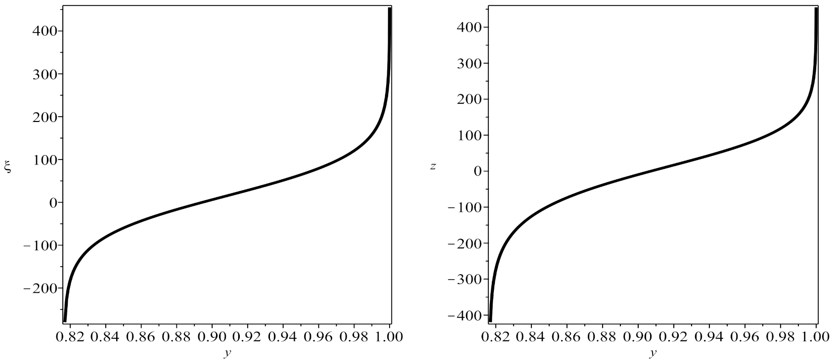
Solution $V\left(\xi \right)$ of Equation (12) can be written as the following

$$\begin{array}{c}V\left(\xi \right)=A_0+\frac{4A_{1}c{\mathrm{e}}^{-\xi \sqrt{c}}}{4ac+b^2+2b{\mathrm{e}}^{-\xi \sqrt{c}}+{\mathrm{e}}^{-2\xi \sqrt{c}}}.\end{array}$$

(42)

At the same time, we find the function $\xi \left(z\right)$ from Equation (18)

$$\begin{array}{c}z=A_0\xi +\frac{2A_1\sqrt{c}}{\sqrt{ac}}arctan\left[\frac{\left(4ac+b^2\right){\mathrm{e}}^{\xi \sqrt{c}}+b}{2\sqrt{ac}}\right]+z_0.\end{array}$$

(43)

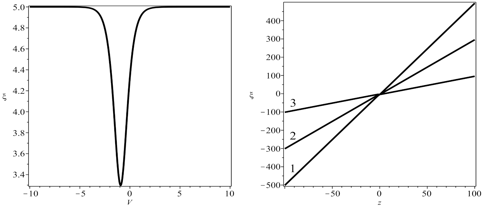
Solution $V\left(\xi \right)$ of Equation (12) is demonstrated in Figure 2 on the left hand side at $A_0=5.0$, $A_1=-2$, $a=2.0$, $b=3.0$ and $c=4.0$. Dependencies $\xi \left(z\right)$ are shown on the right hand side of Figure 2 at $A_0=5.0$, $A_1=-2$, $a=2.0$, $b=3.0$ and $c=4.0$ (curve 1), $A_0=3.0$, $A_1=-2$, $a=2.0$, $b=3.0$ and $c=4.0$ (curve 2) and at $A_0=1.0$, $A_1=-2$, $a=2.0$, $b=3.0$ and $c=4.0$ (curve 3).

Taking into account Equations (8) and (11), we obtain

$$\begin{array}{c}{A}_0+\frac{4A_{1}c{\mathrm{e}}^{-\xi \sqrt{c}}}{4ac+b^2+2b{\mathrm{e}}^{-\xi \sqrt{c}}+{\mathrm{e}}^{-2\xi \sqrt{c}}}-y^{-n}.\end{array}$$

(44)

Solving Equation (44) gives us two expressions for $\xi \left(y\right)$

$$\begin{array}{c}{\xi }_{1,2}\left(y\right)=-\frac{1}{\sqrt{c}}log\left[\frac{A_{1}b{y}^n+2A_{1}c{y}^n\mp 2\sqrt{P}-b}{1-A_{0}y}\right],\end{array}$$

(45)

where P is as follows

$$\begin{array}{c}P=\left(A_1^2{c}^2+A_0{A}_{1}bc-A_0^{2}ac\right)y^{2n}+\left(2A_{0}ac-bc\right)y^n-ac.\end{array}$$

(46)

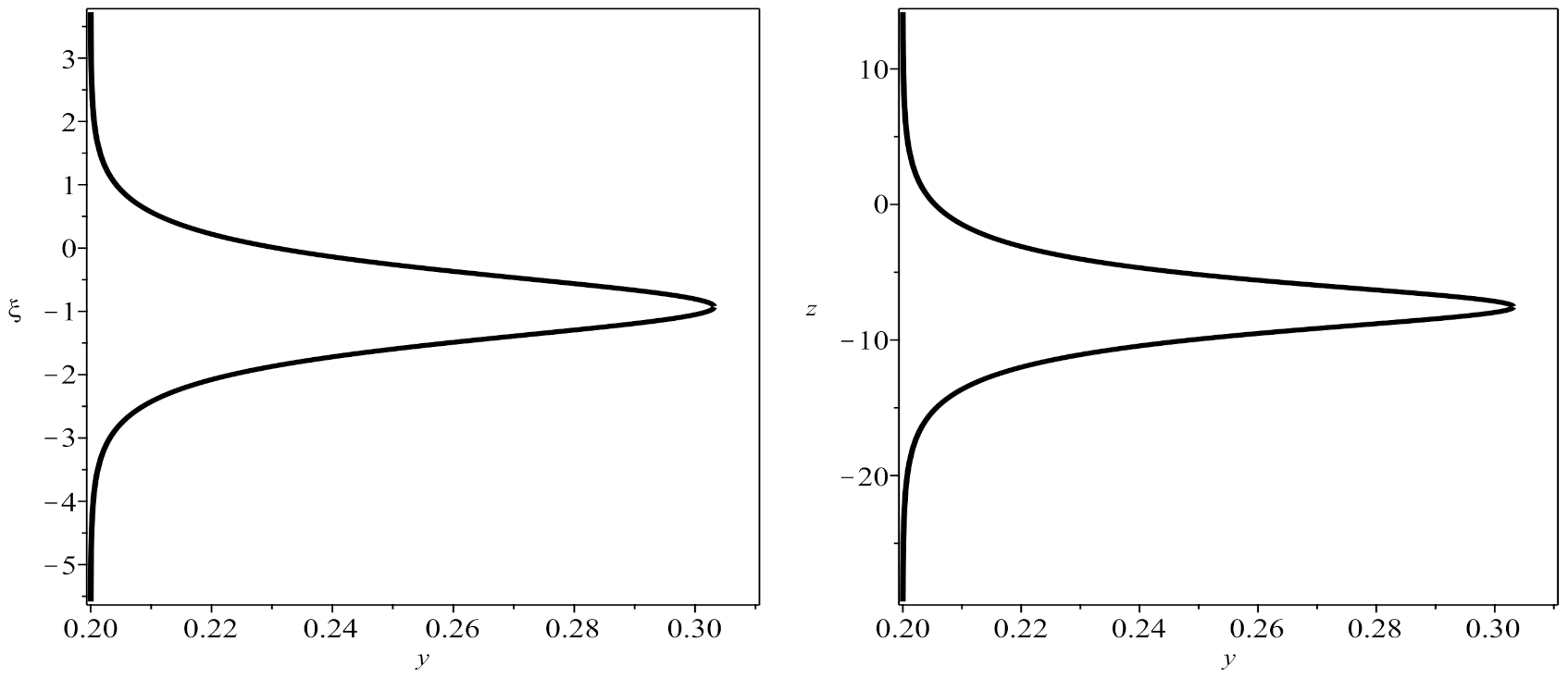
The dependence $\xi \left(y\right)$ is the two-valued function. Equating ${\xi }_1\left(y\right)$ and ${\xi }_2\left(y\right)$, we obtain the following formula for $y^{*}$

$$\begin{array}{c}{y}^{*}={\left[\frac{2A_{0}a-A_{1}b+\sqrt{4ac{A_1}^2+{A_1}^2{b}^2}}{2{A_0}^{2}a-2A_0{A}_{1}b-2{A_1}^{2}c}\right]}^{\frac{1}{n}}.\end{array}$$

(47)

It can be seen that $y^{*}$ depends on the values of $A_0$, $A_1$, a, b and c. by substituting $y^{*}$ into (45) we obtain ${\xi }^{*}$. The dependence $\xi \left(z\right)$ can be written in the form

$$\xi \left(y\right)=\left\{\begin{array}{cc}{\xi }_1\left(y\right),\hfill & \xi >{\xi }^{*},\hfill \\ {\xi }_2\left(y\right),\hfill & \xi <{\xi }^{*}.\hfill \end{array}\right.$$

(48)

Substituting $\xi \left(y\right)$ into expression (43), yields the solitary wave in the form

$$z\left(y\right)=\left\{\begin{array}{cc}{A}_0{\xi }_1\left(y\right)+\frac{2A_1\sqrt{c}}{\sqrt{ac}}arctan\left[\frac{\left(4ac+b^2\right){\mathrm{e}}^{{\xi }_1\left(y\right)\sqrt{c}}+b}{2\sqrt{ac}}\right]+z_0,\hfill & z>z^{*},\hfill \\ A_0{\xi }_2\left(y\right)+\frac{2A_1\sqrt{c}}{\sqrt{ac}}arctan\left[\frac{\left(4ac+b^2\right){\mathrm{e}}^{{\xi }_2\left(y\right)\sqrt{c}}+b}{2\sqrt{ac}}\right]+z_0\hfill & z<z^{*},\hfill \end{array}\right.$$

(49)

where $Z^{*}$ is found taking into account $y^{*}$.

Implicit solitary waves solutions $\xi \left(y\right)$ of Equation (10) (on the left) and $z\left(y\right)$ of Equation (5) are illustrated in Figure 3 at $z_0=0.0$, $A_0=5.0$, $A_1=-2.0$, $n=1$, $a=2.0$, $b=3.0$, and $c=4.0$.

5. Conclusions

In this paper, Equation (1) has been studied. Equation (1) is the generalization of the famous nonlinear Schrödinger equation and can be used for the description of propagation pulses in optical fiber. Using the transformations for dependent and independent variables we have presented the algorithm for construction of exact solutions of nonlinear differential equations. Exact formulas for solitary waves solutions in the form of kinks and optical solitons are given as the implicit functions. The approach for finding exact solutions can be used for some other nonlinear differential equations.

References

- Kudryashov, N.A. Model of propagation pulses in an optical fiber with a new law of refractive indices. Optik 2021, 248, 168160. [Google Scholar] [CrossRef]
- Kudryashov, N.A. A generalized model for description of propagation pulses in optical fiber. Optik 2019, 189, 42–52. [Google Scholar] [CrossRef]
- Kudryashov, N.A. Mathematical model of propagation pulse in optical fiber with power nonlinearities. Optik 2020, 212, 164750. [Google Scholar] [CrossRef]
- Kudryashov, N.A. Solitary wave solutions of hierarchy with non-local nonlinearity. Appl. Math. Lett. 2020, 103, 106155. [Google Scholar] [CrossRef]
- Zayed, E.M.E.; Shohib, R.M.A.; Biswas, A.; Ekici, M.; Triki, H.; Alzahrani, A.K.; Belic, M.R. Optical solitons and other solutions to Kudryashov’s equation with three innovative integration norms. Optik 2020, 211, 164431. [Google Scholar] [CrossRef]
- Arshed, S.; Arif, A. Soliton solutions of higher-order nonlinear schrodinger equation (NLSE) and nonlinear kudryashov’s equation. Optik 2020, 209, 164588. [Google Scholar] [CrossRef]
- Kumar, S.; Malik, S.; Biswas, A.; Zhou, Q.; Moraru, L.; Alzahrani, A.K.; Belic, M.R. Optical Solitons with Kudryashov’s Equation by Lie Symmetry Analysis. Phys. Wave Phenom. 2020, 28, 299–304. [Google Scholar] [CrossRef]
- Yildirim, Y.; Biswas, A.; Ekici, M.; Gonzalez-Gaxiola, O.; Khan, S.; Triki, H.; Moraru, L.; Alzahrani, A.K.; Belic, M.R. Optical solitons with Kudryashov’s model by a range of integration norms. Chin. J. Phys. 2020, 66, 660–672. [Google Scholar] [CrossRef]
- Kudryashov, N.A. Optical solitons of the resonant nonlinear Schrodinger equation with arbitrary index. Optik 2021, 235, 166626. [Google Scholar] [CrossRef]
- Zayed, E.M.E.; Shohib, R.M.A.; Biswas, A.; Ekici, M.; Moraru, L.; Alzahrani, A.K.; Belic, M.R. Optical solitons with differential group delay for Kudryashov’s model by the auxiliary equation mapping method. Chin. J. Phys. 2020, 67, 631–645. [Google Scholar] [CrossRef]
- Zayed, E.M.E.; Alngar, M.E.M.; Biswas, A.; Asma, M.; Ekici, M.; Alzahrani, A.K.; Belic, M.R. Optical solitons and conservation laws with generalized Kudryashov’s law of refractive index. Chaos Solitons Fractals 2020, 139, 110284. [Google Scholar] [CrossRef]
- Zayed, E.M.E.; Alngar, M.E.M.; Biswas, A.; Asma, M.; Ekici, M.; Alzahrani, A.K.; Belic, M.R. Solitons in magneto–optic waveguides with Kudryashov’s law of refractive index. Chaos Solitons Fractals 2020, 140, 110129. [Google Scholar] [CrossRef]
- Kudryashov, N.A. Optical solitons of mathematical model with arbitrary refractive index. Optik 2021, 231, 166443. [Google Scholar] [CrossRef]
- Biswas, A.; Asma, M.; Guggilla, P.; Mullick, L.; Moraru, L.; Ekici, M.; Alzahrani, A.K.; Belic, M.R. Optical soliton perturbation with Kudryashov’s equation by semi–inverse variational principle. Phys. Lett. Sect. A Gen. At. Solid State Phys. 2020, 384, 126830. [Google Scholar] [CrossRef]
- Biswas, A.; Sonmezoglu, A.; Ekici, M.; Alzahrani, A.K.; Belic, M.R. Cubic–Quartic Optical Solitons with Differential Group Delay for Kudryashov’s Model by Extended Trial Function. J. Commun. Technol. Electron. 2020, 65, 1384–1398. [Google Scholar] [CrossRef]
- Arnous, A.H.; Biswas, A.; Ekici, M.; Alzahrani, A.K.; Belic, M.R. Optical solitons and conservation laws of Kudryashov’s equation with improved modified extended tanh-function. Optik 2021, 225, 165406. [Google Scholar] [CrossRef]
- Zayed, E.M.E.; Alngar, M.E.M. Optical soliton solutions for the generalized Kudryashov equation of propagation pulse in optical fiber with power nonlinearities by three integration algorithms. Math. Methods Appl. Sci. 2021, 44, 315–324. [Google Scholar] [CrossRef]
- Hyder, A.A.; Soliman, A.H. Exact solutions of space-time local fractal nonlinear evolution equations generalized comformable derivative approach. Resilts Phys. 2020, 17, 103135. [Google Scholar] [CrossRef]
- Hyder, A.A.; Soliman, A.H. An extended Kudryashov technique for solving stochastic nonlinear models with generalized comformable derivatives. Commun. Nonlinear Sci. Numer. Simul. 2021, 97, 105730. [Google Scholar] [CrossRef]
- Zayed, E.M.E.; Shohib, R.M.A.; Alngar, M.E.M.; Biswas, A.; Kara, A.H.; Dakova, A.; Khan, S.; Alshehri, H.M.; Belic, M.R. Solitons and conservation laws in magneto-optic waveguides with generalized Kudryashov’s equation by the unified auxiliary equation approach. Optik 2021, 245, 167694. [Google Scholar] [CrossRef]
- Ekici, M.; Sonmezoglu, A.; Biswas, A. Stationary optical solitons with Kudryashov’s laws of refractive index. Chaos Solitons Fractals 2021, 151, 111226. [Google Scholar] [CrossRef]
- Yildirim, Y.; Biswas, A.; Kara, A.H.; Ekici, M.; Alzahrani, A.K.; Belic, M.R. Cubic–quartic optical soliton perturbation and conservation laws with generalized Kudryashov’s form of refractive index. J. Opt. 2021, 50, 354–360. [Google Scholar] [CrossRef]
- Biswas, A.; Ekici, M.; Dakova, A.; Khan, S.; Moshokoa, S.P.; Alshehri, H.M.; Belic, M.R. Highly dispersive optical soliton perturbation with Kudryashov’s sextic-power law nonlinear refractive index by semi-inverse variation. Results Phys. 2021, 27, 104539. [Google Scholar] [CrossRef]
- Kudryashov, N.A. Exact solutions of the equation for surface waves in a convecting fluid. Appl. Math. Comput. 2019, 344–345, 97–106. [Google Scholar] [CrossRef]
- Kudryashov, N.A. Method for finding highly dispersive optical solitons of nonlinear differential equations. Optik 2019, 206, 163550. [Google Scholar] [CrossRef]
- Kudryashov, N.A. Highly dispersive optical solitons of the generalized nonlinear eigth-order Scrödinger equation. Optik 2020, 206, 164335. [Google Scholar] [CrossRef]
- Kudryashov, N.A. Exact solutions of the generalized Kuramoto-Sivashinsky equation. Phys. Lett. A 1990, 147, 287–291. [Google Scholar] [CrossRef]
- Parkes, E.J.; Duffy, B.R. An automated tanh-function method for finding solitary wave solutions to non-linear evolution equations. Comput. Phys. Commun. 1996, 98, 288–300. [Google Scholar] [CrossRef]
- Malfliet, W.; Hereman, W. The Tanh method: I Exact solutions of nonlinear evolution and wave equations. Phys. Scr. 1996, 54, 563–568. [Google Scholar] [CrossRef]
- Fan, E. Extended tanh-function method and its applications to nonlinear equations. Phys. Lett. A 2000, 227, 212–218. [Google Scholar] [CrossRef]
- Fu, Z.; Liu, S.; Liu, S.; Zhao, Q. New Jacobi elliptic function expansion and new periodic solutions of nonlinear wave equations. Phys. Lett. A 2001, 290, 72–76. [Google Scholar] [CrossRef]
- Liu, S.; Fu, Z.; Liu, S.; Zhao, Q. Jacobi elliptic function expansion method and periodic wave solutions of nonlinear wave equations. Phys. Lett. A 2001, 289, 69–74. [Google Scholar] [CrossRef]
- Biswas, A. 1-soliton solution of the generalized Radhakrishnan–Kundu–Laksmanan equation. Phys. Lett. A 2009, 373, 2546–2548. [Google Scholar] [CrossRef]
- Vitanov, N.K. Application of simplest equations of Bernoulli and Riccati kind for obtaining exact traveling-wave solutions for a class of PDEs with polynomial nonlinearity. Commun. Nonlinear Sci. Numer. Simul. 2010, 15, 2050–2060. [Google Scholar] [CrossRef]
- Vitanov, N.K. Modified method of simplest equation: Powerful tool for obtaining exact and approximate traveling-wave solutions of nonlinear PDEs. Commun. Nonlinear Sci. Numer. Simul. 2011, 16, 1176–1185. [Google Scholar] [CrossRef]
- Vitanov, N.K.; Dimitrova, Z.I.; Kantz, H. Modified method of simplest equation and its application to nonlinear PDEs. Appl. Math. Comput. 2010, 216, 2587–2595. [Google Scholar] [CrossRef]
- Kudryashov, N.A. One method for finding exact solutions of nonlinear differential equations. Commun. Nonlinear Sci. Numer. Simul. 2012, 17, 2248–2253. [Google Scholar] [CrossRef] [Green Version]
- Yildirim, Y.; Biswas, A.; Kara, A.H.; Guggilla, P.; Khan, S.; Alzahrani, A.K.; Belic, M.R. Highly dispersive optical solitons and conservation laws with Kudryashov’s sextic power-law of nonlinear refractive index. Optik 2021, 240, 166915. [Google Scholar] [CrossRef]
- Elsherbeny, A.M.; El-Barkouky, R.; Ahmed, H.M.; Arnous, A.H.; El-Hassani, R.M.I.; Biswas, A.; Yildirim, Y.; Alshomrani, A.S. Optical soliton perturbation with Kudryashov’s generalized nonlinear refractive index. Optik 2021, 240, 166620. [Google Scholar] [CrossRef]
- Zayed, E.M.E.; Alngar, M.E.M.; Biswas, A.; Kara, A.H.; Asma, M.; Ekici, M.; Khan, S.; Alzahrani, A.K.; Belic, M.R. Solitons and conservation laws in magneto–optic waveguides with generalized Kudryashov’s equation. Chin. J. Phys. 2021, 69, 186–205. [Google Scholar] [CrossRef]
- Zayed, E.M.E.; Shohib, R.M.A.; Alngar, M.E.M.; Biswas, A.; Ekici, M.; Khan, S.; Alzahrani, A.K.; Belic, M.R. Optical solitons and conservation laws associated with Kudryashov’s sextic power-law nonlinearity of refractive index. Ukr. J. Phys. Opt. 2021, 22, 38–49. [Google Scholar] [CrossRef]
- Zayed, E.M.E.; Alngar, M.E.M.; Biswas, A.; Ekici, M.; Alzahrani, A.K.; Belic, M.R. Chirped and Chirp-Free Optical Solitons in Fiber Bragg Gratings with Kudryashov’s Model in Presence of Dispersive Reflectivity. J. Commun. Technol. Electron. 2020, 65, 1267–1287. [Google Scholar] [CrossRef]
- Arnous, A.H.; Zhou, Q.; Biswas, A.; Guggilla, P.; Khan, S.; Yildirim, Y.; Alshomrani, A.S.; Alshehri, H.M. Optical solitons in fiber Bragg gratings with cubic-quartic dispersive reflectivity by enhanced Kudryashov’s approach. Phys. Lett. A 2022, 422, 127797. [Google Scholar] [CrossRef]
- Gonzalez-Gaxiola, O. Optical soliton solutions for Triki-Biswas equation by Kudryashov’s R function method. Optik 2022, 249, 168230. [Google Scholar] [CrossRef]
- Arnous, A.H. Optical solitons with Biswas-Milovic equation in magneto-optic waveguide having Kudryashov’s aw of refractive index. Optik 2021, 247, 167987. [Google Scholar] [CrossRef]
- Alotaibi, H. Traveling wave solutions to the nonlinear evolution equation using expansion method and addendum to Kudryashov’s method. Symmetry 2021, 13, 2126. [Google Scholar] [CrossRef]
- Kudryashov, N.A. Highly dispersive solitary wave solutions of perturbed nonlinear Schrödinger equations. Appl. Math. Comput. 2020, 371, 124972. [Google Scholar] [CrossRef]
- Raza, N.; Seadawy, A.R.; Kaplan, M.; Butt, A.R. Symbolic computation and sensitivity analysis of nonlinear Kudryashov’s dynamical equation with applications. Phys. Scr. 2021, 96, 105216. [Google Scholar] [CrossRef]
- Kaplan, M.; Akbulut, A. The analysis of the soliton-type solutions of conformable equations by using generalized Kudryashov method. Opt. Quantum Electron. 2021, 53, 498. [Google Scholar] [CrossRef]
- Malik, S.; Kumar, S.; Biswas, A.; Ekici, M.; Dakova, A.; Alzahrani, A.K.; Belic, M.R. Optical solitons and bifurcation analysis in fiber Bragg gratings with Lie symmetry and Kudryashov’s approach. Nonlinear Dyn. 2021, 105, 735–751. [Google Scholar] [CrossRef]
- Rahman, Z.; Ali, M.Z.; Roshid, H.-O. Closed form soliton solutions of three nonlinear fractional models through proposed improved Kudryashov method. Chin. Phys. B 2021, 30, 050202. [Google Scholar] [CrossRef]
Publisher’s Note: MDPI stays neutral with regard to jurisdictional claims in published maps and institutional affiliations. |
© 2021 by the author. Licensee MDPI, Basel, Switzerland. This article is an open access article distributed under the terms and conditions of the Creative Commons Attribution (CC BY) license (https://creativecommons.org/licenses/by/4.0/).