
Integrate-and-Differentiate Approach to Nonlinear System Identification


Abstract
:1. Introduction
2. Identification of Mechanical Systems Using Least Squares
2.1. Least Squares for ODE Reconstruction
| Algorithm 1: Iteratively reweighted least squares (IRLS) with -regularization |
Input: , . Output: . Initialization: , , 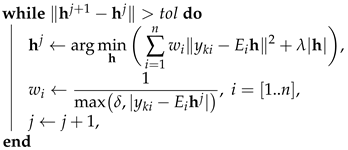 . |
2.2. Mechanical System Identification
| Algorithm 2: DIA for parametric identification of piece-wise linear mechanical system |
Input: , , , Output: . Initialization: 1. Set incidence vectors 2. Find 3. Calculate 4. . 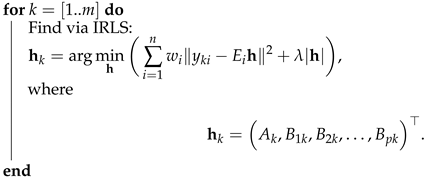 |
| Algorithm 3: IDA for parametric identification of piece-wise linear mechanical system |
Input: , , , , Output: . Initialization: 1. Set incidence vectors 2. Find 3. . 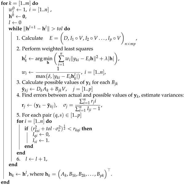 |
3. Study of Chaotic Mechanical System with Backlash
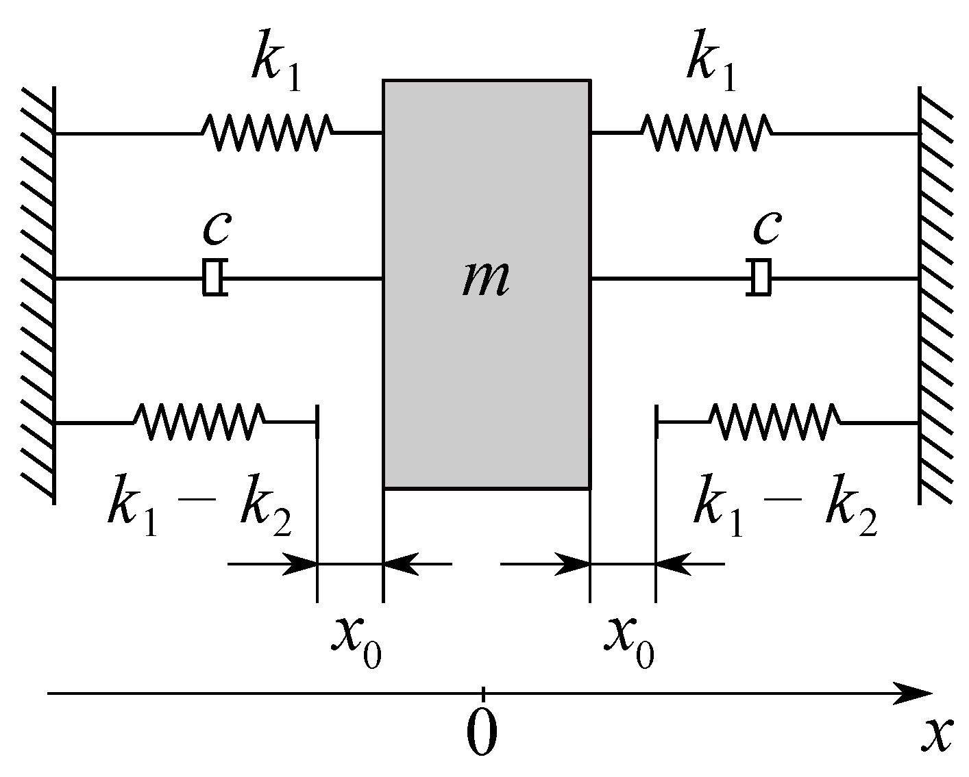
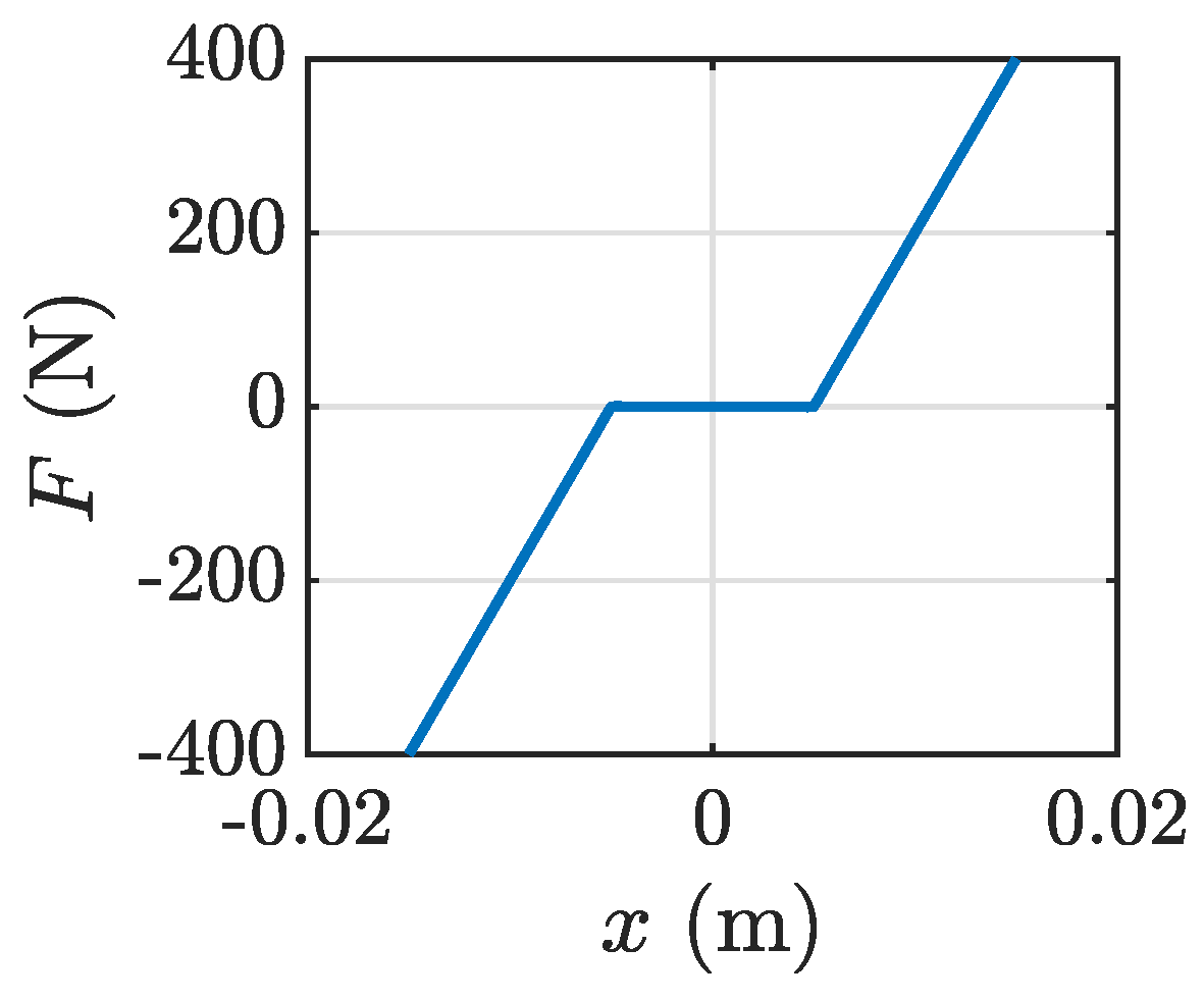
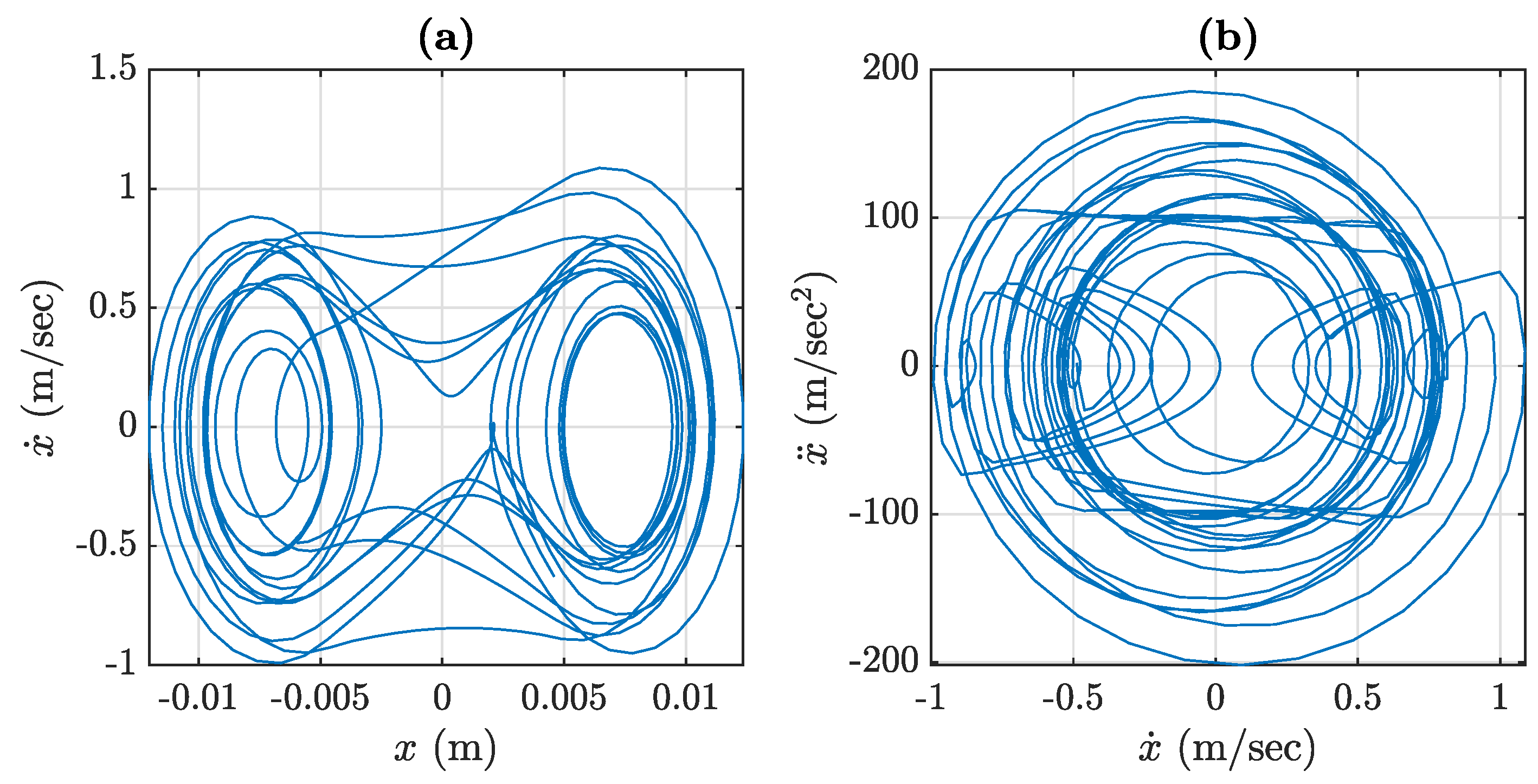
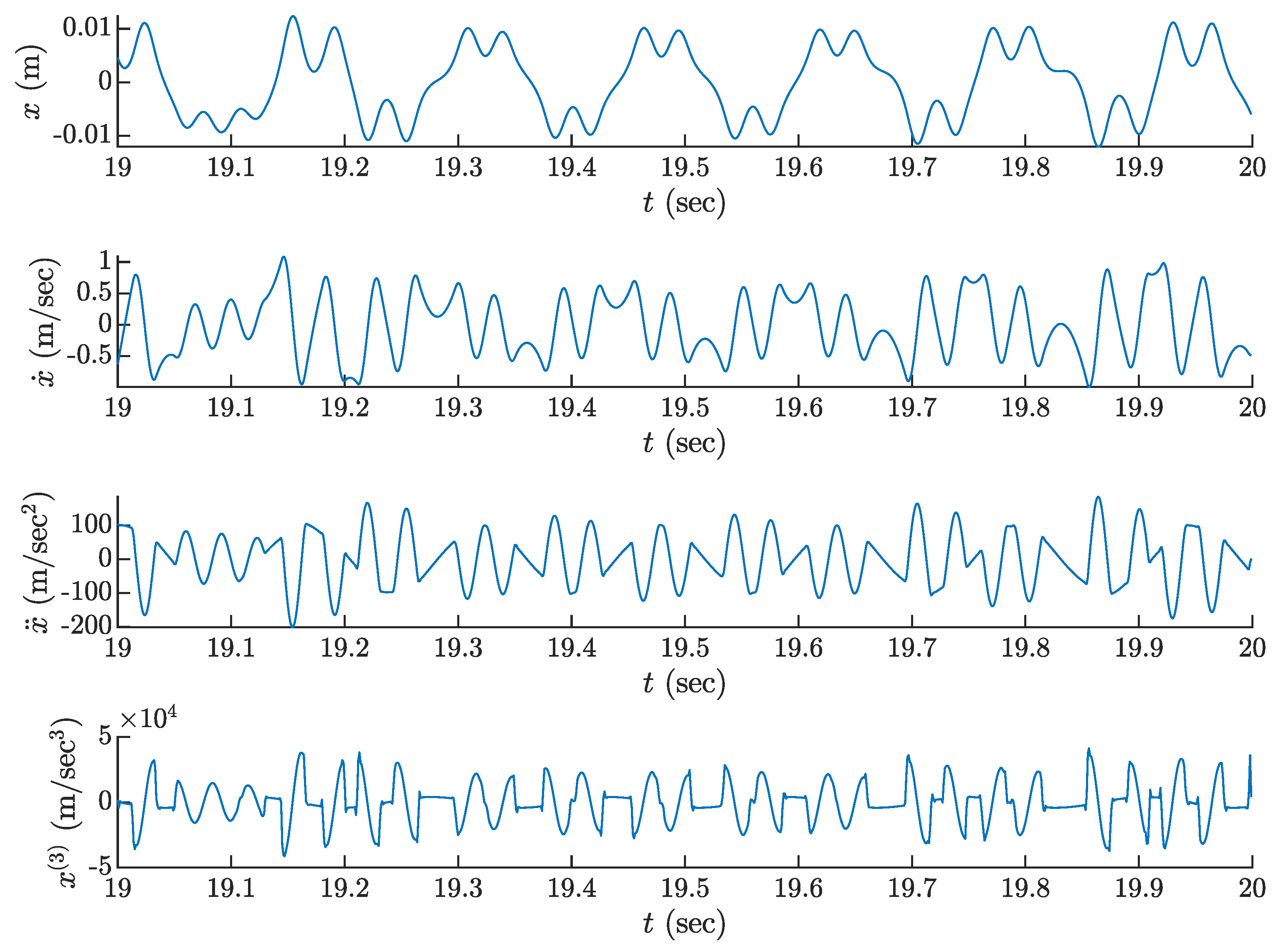
3.1. Lin-Ewins Mechanical Oscillator
3.2. Identification of Nonlinear Stiffness in Lin-Ewins Oscillator
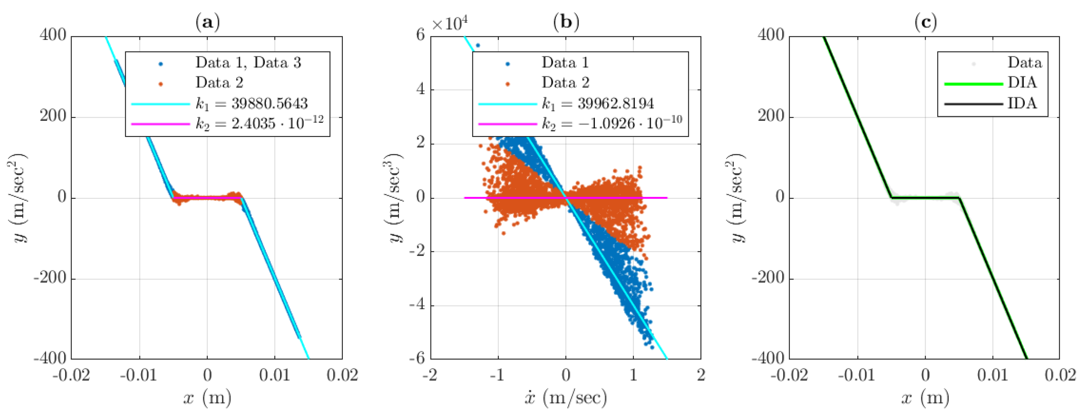
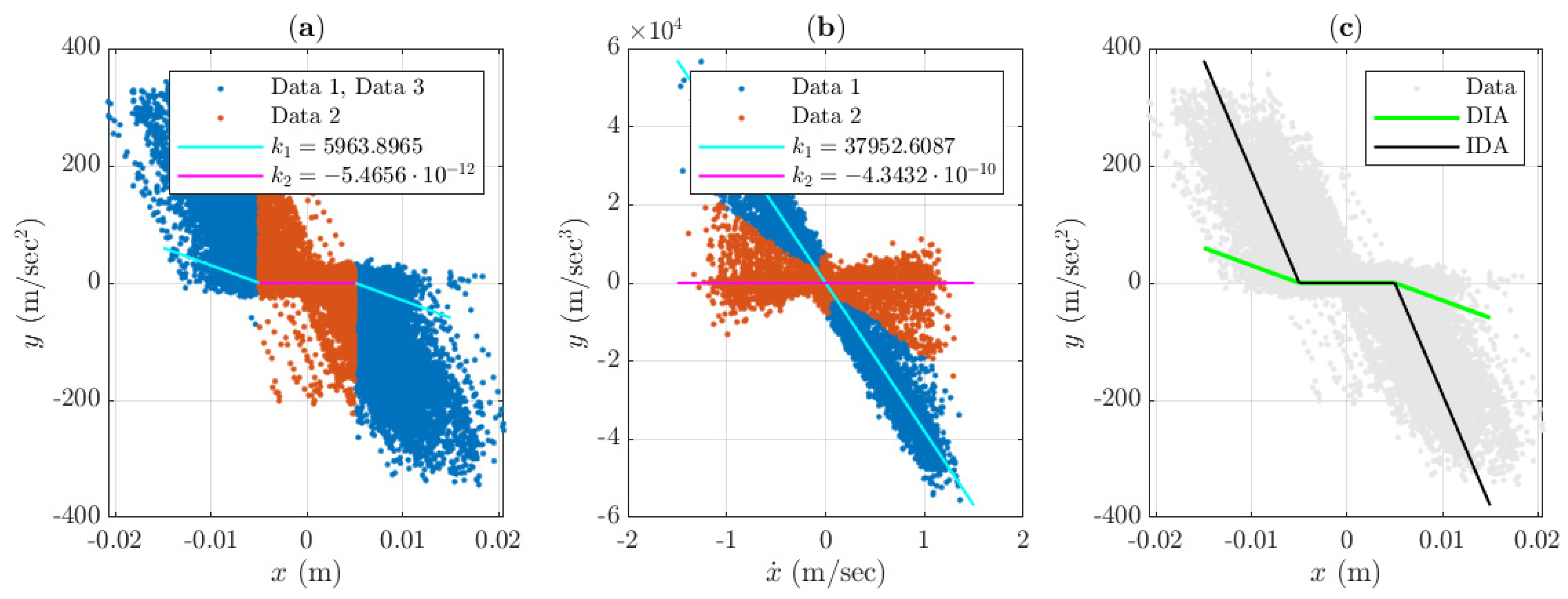
3.2.1. Noiseless Case
3.2.2. Case of Additive Gaussian Noise
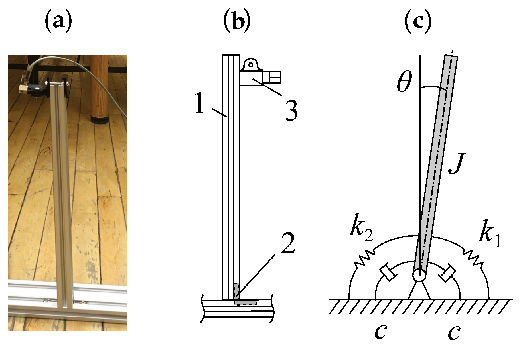
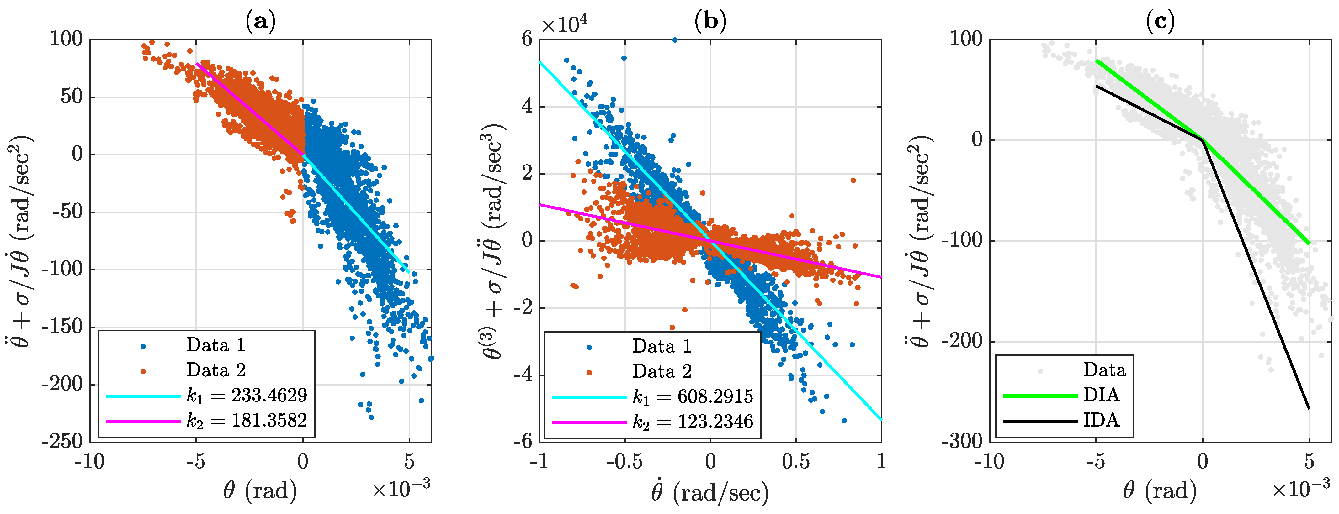
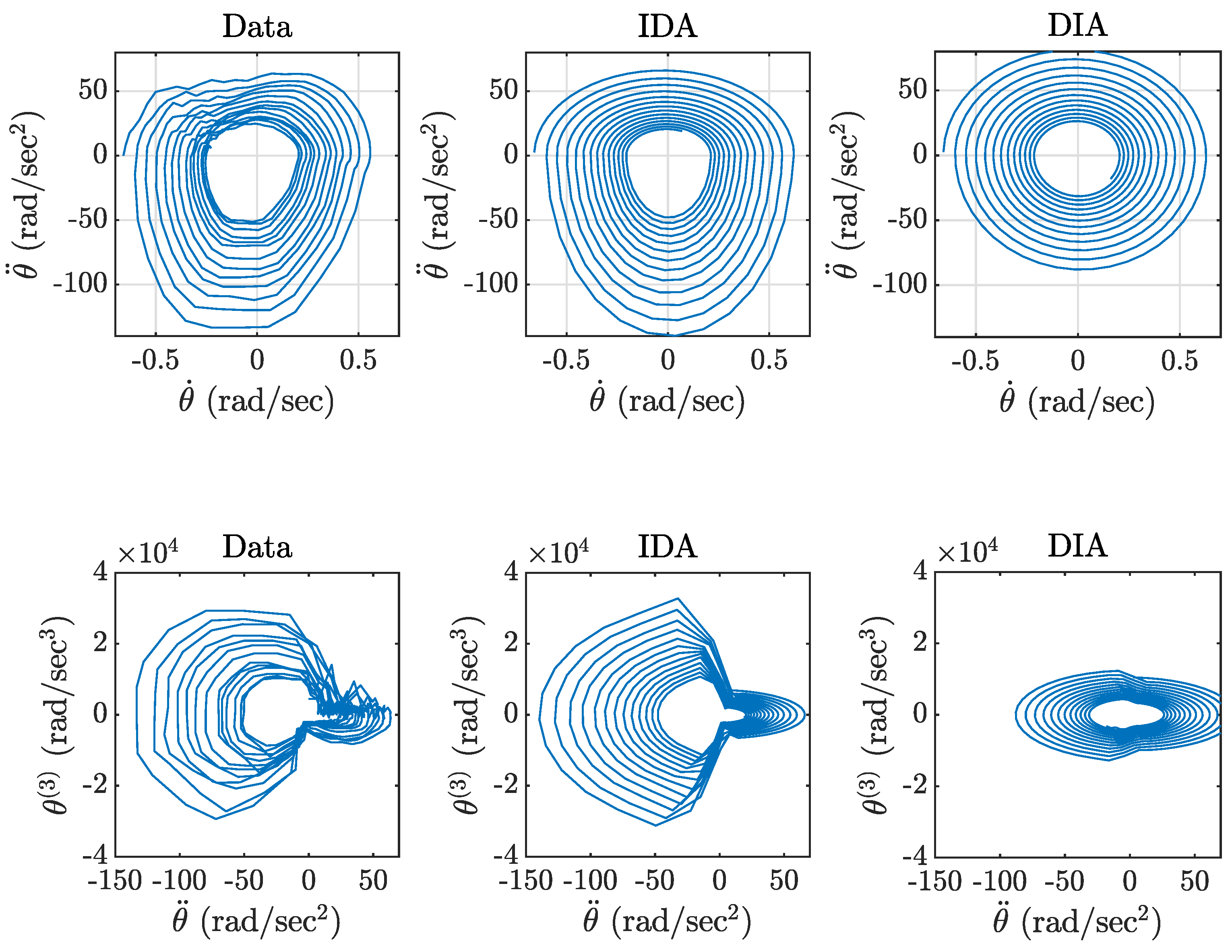
4. Experimental Study of Nonlinear Vibration of an Aluminum Beam
5. Conclusions and Discussion
Author Contributions
Funding
Institutional Review Board Statement
Informed Consent Statement
Conflicts of Interest
Abbreviations
| ODE | Ordinary Differential Equation |
| OLS | Ordinary Least Squares |
| IRLS | Iteratively Reweighted Least Squares |
| DIA | Double Integration Approach |
| IDA | Integrate-and-Differentiate Approach |
References
- Kera, H.; Hasegawa, Y. Noise-tolerant algebraic method for reconstruction of nonlinear dynamical systems. Nonlinear Dyn. 2016, 85, 675–692. [Google Scholar] [CrossRef]
- Obeid, S.; Ahmadi, G.; Jha, R. NARMAX Identification Based Closed-Loop Control of Flow Separation over NACA 0015 Airfoil. Fluids 2020, 5, 100. [Google Scholar] [CrossRef]
- Tian, R.; Yang, Y.; van der Helm, F.C.; Dewald, J. A novel approach for modeling neural responses to joint perturbations using the NARMAX method and a hierarchical neural network. Front. Comput. Neurosci. 2018, 12, 96. [Google Scholar] [CrossRef] [Green Version]
- Brusaferri, A.; Matteucci, M.; Portolani, P.; Spinelli, S. Nonlinear system identification using a recurrent network in a Bayesian framework. In Proceedings of the 2019 IEEE 17th International Conference on Industrial Informatics, Helsinki-Espoo, Finland, 22–25 July 2019; Volume 1, pp. 319–324. [Google Scholar]
- Yang, L.; Liu, J.; Yan, R.; Chen, X. Spline adaptive filter with arctangent-momentum strategy for nonlinear system identification. Signal Process. 2019, 164, 99–109. [Google Scholar] [CrossRef]
- Gedon, D.; Wahlström, N.; Schön, T.B.; Ljung, L. Deep state space models for nonlinear system identification. IFAC-PapersOnLine 2021, 54, 481–486. [Google Scholar] [CrossRef]
- Karimshoushtari, M.; Novara, C. Design of experiments for nonlinear system identification: A set membership approach. Automatica 2020, 119, 109036. [Google Scholar] [CrossRef]
- Davila, J.; Fridman, L.; Poznyak, A. Observation and Identification of Mechanical Systems via Second Order Sliding Modes. Int. J. Control 2006, 79, 232–237. [Google Scholar] [CrossRef] [Green Version]
- Kok, M.; Hol, J.D.; Schön, T.B. Using Inertial Sensors for Position and Orientation Estimation. Found. Trends Signal Process. 2017, 11, 1–153. [Google Scholar] [CrossRef] [Green Version]
- Karimov, A.; Nepomuceno, E.G.; Tutueva, A.; Butusov, D. Algebraic method for the reconstruction of partially observed nonlinear systems using differential and integral embedding. Mathematics 2020, 8, 300. [Google Scholar] [CrossRef] [Green Version]
- Singh, A.; Moore, K.J. Characteristic nonlinear system identification of local attachments with clearance nonlinearities. Nonlinear Dyn. 2020, 102, 1667–1684. [Google Scholar] [CrossRef]
- Pham, M.T.; Gautier, M.; Poignet, P. Accelerometer based identification of mechanical systems. In Proceedings of the 2002 IEEE International Conference on Robotics and Automation, Washington, DC, USA, 11–15 May 2002; Volume 4, pp. 4293–4298. [Google Scholar]
- Ewald, V.; Venkat, R.S.; Asokkumar, A.; Benedictus, R.; Boller, C.; Groves, R.M. Perception modelling by invariant representation of deep learning for automated structural diagnostic in aircraft maintenance: A study case using DeepSHM. Mech. Syst. Signal Process. 2021, 165, 108153. [Google Scholar] [CrossRef]
- Peng, G.C.; Alber, M.; Tepole, A.B.; Cannon, W.R.; De, S.; Dura-Bernal, S.; Garikipati, K.; Karniadakis, G.; Lytton, W.W.; Perdikaris, P.; et al. Multiscale modeling meets machine learning: What can we learn? Arch. Comput. Methods Eng. 2021, 28, 1017–1037. [Google Scholar] [CrossRef] [Green Version]
- Hanke, S.; Peitz, S.; Wallscheid, O.; Böcker, J.; Dellnitz, M. Finite-control-set model predictive control for a permanent magnet synchronous motor application with online least squares system identification. In Proceedings of the 2019 IEEE International Symposium on Predictive Control of Electrical Drives and Power Electronics, Quanzhou, China, 31 May–2 June 2019; pp. 1–6. [Google Scholar]
- Galrinho, M. Least Squares Methods for System Identification of Structured Models. Ph.D. Thesis, KTH Royal Institute of Technology, Stockholm, Sweden, 2016. [Google Scholar]
- Elisei-Iliescu, C.; Paleologu, C.; Benesty, J.; Stanciu, C.; Anghel, C.; Ciochină, S. Recursive least-squares algorithms for the identification of low-rank systems. IEEE/ACM Trans. Audio Speech Lang. Process. 2019, 27, 903–918. [Google Scholar] [CrossRef]
- Tierney, C.; Mulgrew, B. Adaptive waveform design with least-squares system identification for interference mitigation in SAR. In Proceedings of the 2017 IEEE Radar Conference (RadarConf), Seattle, WA, USA, 8–12 May 2017; pp. 180–185. [Google Scholar]
- Xia, B.; Zhao, X.; De Callafon, R.; Garnier, H.; Nguyen, T.; Mi, C. Accurate Lithium-ion battery parameter estimation with continuous-time system identification methods. Appl. Energy 2016, 179, 426–436. [Google Scholar] [CrossRef] [Green Version]
- Ljung, L. Consistency of the least-squares identification method. IEEE Trans. Autom. Control 1976, 21, 779–781. [Google Scholar] [CrossRef]
- Manikantan, R.; Chakraborty, S.; Uchida, T.K.; Vyasarayani, C. Parameter identification in nonlinear mechanical systems with noisy partial state measurement using PID-controller penalty functions. Mathematics 2020, 8, 1084. [Google Scholar] [CrossRef]
- Bian, Q.; Zhao, K.; Wang, X.; Xie, R. System identification method for small unmanned helicopter based on improved particle swarm optimization. J. Bionic Eng. 2016, 13, 504–514. [Google Scholar] [CrossRef]
- Cortez-Vega, R.; Maldonado, J.; Garrido, R. Parameter Identification using PSO under measurement noise conditions. In Proceedings of the 2019 6th International Conference on Control, Decision and Information Technologies, Le Cnam, Paris, 23–26 April 2019; pp. 103–108. [Google Scholar]
- Kommenda, M.; Burlacu, B.; Kronberger, G.; Affenzeller, M. Parameter identification for symbolic regression using nonlinear least squares. Genet. Program. Evolvable Mach. 2020, 21, 471–501. [Google Scholar] [CrossRef] [Green Version]
- Brunton, S.L.; Proctor, J.L.; Kutz, J.N. Discovering governing equations from data by sparse identification of nonlinear dynamical systems. Proc. Natl. Acad. Sci. USA 2016, 113, 3932–3937. [Google Scholar] [CrossRef] [Green Version]
- Mateos, G.; Giannakis, G.B. Robust nonparametric regression via sparsity control with application to load curve data cleansing. IEEE Trans. Signal Process. 2011, 60, 1571–1584. [Google Scholar] [CrossRef] [Green Version]
- Daubechies, I.; DeVore, R.; Fornasier, M.; Güntürk, C.S. Iteratively reweighted least squares minimization for sparse recovery. Commun. Pure Appl. Math. A J. Issued Courant Inst. Math. Sci. 2010, 63, 1–38. [Google Scholar] [CrossRef] [Green Version]
- Kümmerle, C.; Mayrink Verdun, C.; Stöger, D. Iteratively Reweighted Least Squares for ℓ1-minimization with Global Linear Convergence Rate. arXiv 2020, arXiv:2012.12250. [Google Scholar]
- Xie, L.; Zhou, Z.; Zhao, L.; Wan, C.; Tang, H.; Xue, S. Parameter identification for structural health monitoring with extended Kalman filter considering integration and noise effect. Appl. Sci. 2018, 8, 2480. [Google Scholar] [CrossRef] [Green Version]
- Huang, G.P.; Mourikis, A.I.; Roumeliotis, S.I. Analysis and improvement of the consistency of extended Kalman filter based SLAM. In Proceedings of the 2008 IEEE International Conference on Robotics and Automation, Pasadena, CA, USA, 22–25 May 2008; pp. 473–479. [Google Scholar]
- Nordin, M.; Gutman, P.O. Controlling mechanical systems with backlash—A survey. Automatica 2002, 38, 1633–1649. [Google Scholar] [CrossRef]
- Yao, H.; Cao, Y.; Zhang, S.; Wen, B. A novel energy sink with piecewise linear stiffness. Nonlinear Dyn. 2018, 94, 2265–2275. [Google Scholar] [CrossRef] [Green Version]
- Wang, Y. Dynamics of unsymmetric piecewise-linear/non-linear systems using finite elements in time. J. Sound Vib. 1995, 185, 155–170. [Google Scholar] [CrossRef] [Green Version]
- Levien, R.; Tan, S. Double pendulum: An experiment in chaos. Am. J. Phys. 1993, 61, 1038–1044. [Google Scholar] [CrossRef]
- Lin, R.; Ewins, D. Chaotic vibration of mechanical systems with backlash. Mech. Syst. Signal Process. 1993, 7, 257–272. [Google Scholar] [CrossRef]
- Korobiichuk, I. Analysis of Errors of Piezoelectric Sensors used in Weapon Stabilizers. Metrol. Meas. Syst. 2017, 24, 91–100. [Google Scholar] [CrossRef]
- Bosch Rexroth. Basic Mechanic Elements. Available online: https://www.boschrexroth.com/en/xc/products/product-groups/assembly-technology/basic-mechanic-elements (accessed on 8 September 2021).
- Karimov, T.; Butusov, D.; Andreev, V.; Karimov, A.; Tutueva, A. Accurate synchronization of digital and analog chaotic systems by parameters re-identification. Electronics 2018, 7, 123. [Google Scholar] [CrossRef] [Green Version]
- Karimov, A.; Tutueva, A.; Karimov, T.; Druzhina, O.; Butusov, D. Adaptive generalized synchronization between circuit and computer implementations of the Rössler system. Appl. Sci. 2021, 11, 81. [Google Scholar] [CrossRef]
- Tutueva, A.V.; Nepomuceno, E.G.; Karimov, A.I.; Andreev, V.S.; Butusov, D.N. Adaptive chaotic maps and their application to pseudo-random numbers generation. Chaos Solitons Fractals 2020, 133, 109615. [Google Scholar] [CrossRef]
- Chang, R.J.; Wang, Y.C. Experimental Investigation on the Lumped Model of Nonlinear Rocker–Rocker Mechanism with Flexible Coupler. J. Dyn. Syst. Meas. Control 2020, 142, 061004. [Google Scholar] [CrossRef]


| Approach | Estimated | Relative Error of | Estimated |
|---|---|---|---|
| DIA, without noise | 39,880.6 | 0.0030 | |
| IDA, without noise | 39,962.3 | 0.0009 | |
| DIA, with noise | 5963.9 | 0.85 | |
| IDA, with noise | 37,952.6 | 0.05 |
| Approach | Estimated | Estimated |
|---|---|---|
| DIA | 233.5 | 181.6 |
| IDA | 608.3 | 123.2 |
Publisher’s Note: MDPI stays neutral with regard to jurisdictional claims in published maps and institutional affiliations. |
© 2021 by the authors. Licensee MDPI, Basel, Switzerland. This article is an open access article distributed under the terms and conditions of the Creative Commons Attribution (CC BY) license (https://creativecommons.org/licenses/by/4.0/).
Share and Cite
Karimov, A.I.; Kopets, E.; Nepomuceno, E.G.; Butusov, D. Integrate-and-Differentiate Approach to Nonlinear System Identification. Mathematics 2021, 9, 2999. https://doi.org/10.3390/math9232999
Karimov AI, Kopets E, Nepomuceno EG, Butusov D. Integrate-and-Differentiate Approach to Nonlinear System Identification. Mathematics. 2021; 9(23):2999. https://doi.org/10.3390/math9232999
Chicago/Turabian StyleKarimov, Artur I., Ekaterina Kopets, Erivelton G. Nepomuceno, and Denis Butusov. 2021. "Integrate-and-Differentiate Approach to Nonlinear System Identification" Mathematics 9, no. 23: 2999. https://doi.org/10.3390/math9232999
APA StyleKarimov, A. I., Kopets, E., Nepomuceno, E. G., & Butusov, D. (2021). Integrate-and-Differentiate Approach to Nonlinear System Identification. Mathematics, 9(23), 2999. https://doi.org/10.3390/math9232999