
Boosting Atomic Orbit Search Using Dynamic-Based Learning for Feature Selection

 ,
,  ,
,  ,
,  ,
,  ,
,  ,
,  and
and
Abstract
:1. Introduction
- We propose an alternative feature selection method to improve the behavior of atomic Orbit optimization (AOS).
- We use the dynamic opposite-based learning to enhance the exploration and maintain the diversity of solutions during the searching process.
- We compare the performance of the developed AOSD with other MH techniques using different datasets.
2. Related Works
3. Background
3.1. Atomic Orbital Search
3.2. Dynamic-Opposite Learning
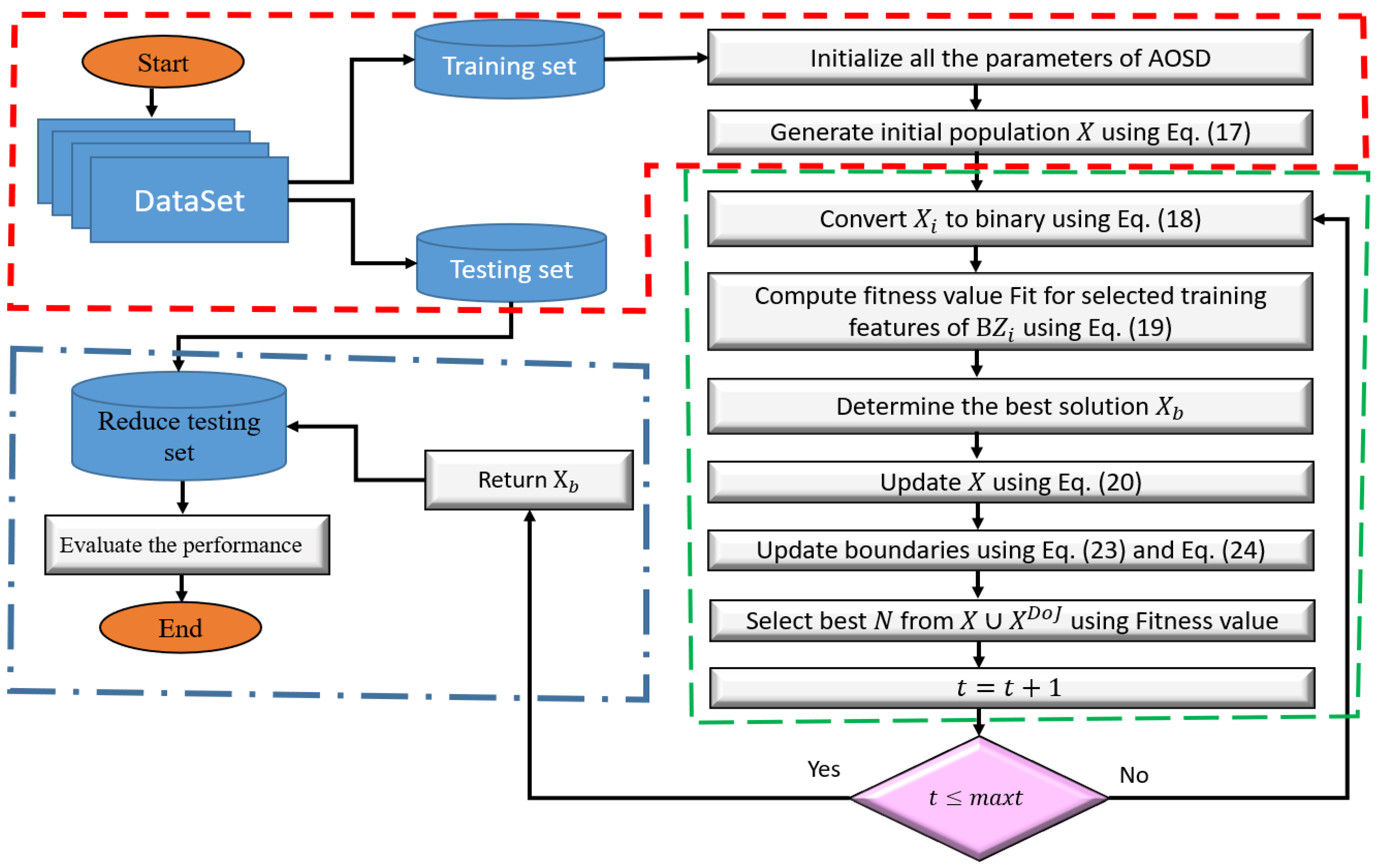
4. Developed AOSD Feature Selection Algorithm
4.1. Learning Phase
4.2. Evaluation Phase
5. Experimental Results
5.1. Experimental Datasets and Parameter Settings
5.2. Performance Measures
- Average accuracy : This measure is the rate of correctly data classification, and it is computed as [22,55,56,57]:Each method is performed 30 times (); thus, the is computed as:
- Standard deviation (STD): STD is employed to assess the quality of each applied method and analyze the achieved results in different runs. It is computed as [22,55,56,57]:(Note: is computed for each metric: Accuracy, Fitness, Time, Number of selected features, Sensitivity, and Specificity.
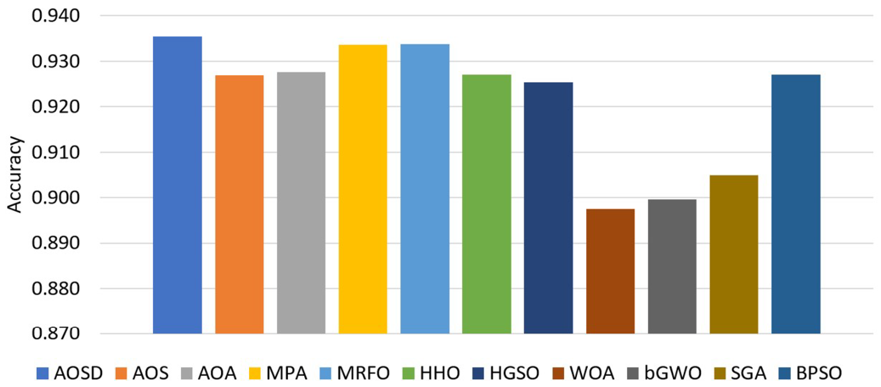
5.3. Comparisons
6. Conclusions
Author Contributions
Funding
Institutional Review Board Statement
Informed Consent Statement
Acknowledgments
Conflicts of Interest
References
- Tubishat, M.; Idris, N.; Shuib, L.; Abushariah, M.A.; Mirjalili, S. Improved Salp Swarm Algorithm based on opposition based learning and novel local search algorithm for feature selection. Expert Syst. Appl. 2020, 145, 113122. [Google Scholar] [CrossRef]
- Shao, Z.; Wu, W.; Li, D. Spatio-temporal-spectral observation model for urban remote sensing. Geo-Spat. Inf. Sci. 2021, 17, 372–386. [Google Scholar] [CrossRef]
- Ibrahim, R.A.; Ewees, A.A.; Oliva, D.; Abd Elaziz, M.; Lu, S. Improved salp swarm algorithm based on particle swarm optimization for feature selection. J. Ambient Intell. Humaniz. Comput. 2019, 10, 3155–3169. [Google Scholar] [CrossRef]
- Zebari, R.; Abdulazeez, A.; Zeebaree, D.; Zebari, D.; Saeed, J. A comprehensive review of dimensionality reduction techniques for feature selection and feature extraction. J. Appl. Sci. Technol. Trends 2020, 1, 56–70. [Google Scholar] [CrossRef]
- Venkatesh, B.; Anuradha, J. A review of feature selection and its methods. Cybern. Inf. Technol. 2019, 19, 3–26. [Google Scholar] [CrossRef] [Green Version]
- Shao, Z.; Sumari, N.S.; Portnov, A.; Ujoh, F.; Musakwa, W.; Mandela, P.J. Urban sprawl and its impact on sustainable urban development: A combination of remote sensing and social media data. Geo-Spat. Inf. Sci. 2021, 24, 241–255. [Google Scholar] [CrossRef]
- Abdel-Basset, M.; Ding, W.; El-Shahat, D. A hybrid Harris Hawks optimization algorithm with simulated annealing for feature selection. Artif. Intell. Rev. 2021, 54, 593–637. [Google Scholar] [CrossRef]
- El-Hasnony, I.M.; Barakat, S.I.; Elhoseny, M.; Mostafa, R.R. Improved feature selection model for big data analytics. IEEE Access 2020, 8, 66989–67004. [Google Scholar] [CrossRef]
- Deng, X.; Li, Y.; Weng, J.; Zhang, J. Feature selection for text classification: A review. Multimed. Tools Appl. 2019, 78, 3. [Google Scholar] [CrossRef]
- Ewees, A.A.; Abualigah, L.; Yousri, D.; Algamal, Z.Y.; Al-qaness, M.A.; Ibrahim, R.A.; Abd Elaziz, M. Improved Slime Mould Algorithm based on Firefly Algorithm for feature selection: A case study on QSAR model. Eng. Comput. 2021, 31, 1–15. [Google Scholar]
- Alex, S.B.; Mary, L.; Babu, B.P. Attention and Feature Selection for Automatic Speech Emotion Recognition Using Utterance and Syllable-Level Prosodic Features. Circuits, Syst. Signal Process. 2020, 39, 11. [Google Scholar] [CrossRef]
- Benazzouz, A.; Guilal, R.; Amirouche, F.; Slimane, Z.E.H. EMG Feature selection for diagnosis of neuromuscular disorders. In Proceedings of the 2019 International Conference on Networking and Advanced Systems (ICNAS), Annaba, Algeria, 26–27 June 2019; pp. 1–5. [Google Scholar]
- Al-qaness, M.A. Device-free human micro-activity recognition method using WiFi signals. Geo-Spat. Inf. Sci. 2019, 22, 128–137. [Google Scholar] [CrossRef]
- Yousri, D.; Abd Elaziz, M.; Abualigah, L.; Oliva, D.; Al-Qaness, M.A.; Ewees, A.A. COVID-19 X-ray images classification based on enhanced fractional-order cuckoo search optimizer using heavy-tailed distributions. Appl. Soft Comput. 2021, 101, 107052. [Google Scholar] [CrossRef]
- Nadimi-Shahraki, M.H.; Banaie-Dezfouli, M.; Zamani, H.; Taghian, S.; Mirjalili, S. B-MFO: A Binary Moth-Flame Optimization for Feature Selection from Medical Datasets. Computers 2021, 10, 136. [Google Scholar] [CrossRef]
- Hancer, E. A new multi-objective differential evolution approach for simultaneous clustering and feature selection. Eng. Appl. Artif. Intell. 2020, 87, 103307. [Google Scholar] [CrossRef]
- Amini, F.; Hu, G. A two-layer feature selection method using genetic algorithm and elastic net. Expert Syst. Appl. 2021, 166, 114072. [Google Scholar] [CrossRef]
- Song, X.f.; Zhang, Y.; Gong, D.w.; Sun, X.y. Feature selection using bare-bones particle swarm optimization with mutual information. Pattern Recognit. 2021, 112, 107804. [Google Scholar] [CrossRef]
- Tubishat, M.; Ja’afar, S.; Alswaitti, M.; Mirjalili, S.; Idris, N.; Ismail, M.A.; Omar, M.S. Dynamic salp swarm algorithm for feature selection. Expert Syst. Appl. 2021, 164, 113873. [Google Scholar] [CrossRef]
- Sathiyabhama, B.; Kumar, S.U.; Jayanthi, J.; Sathiya, T.; Ilavarasi, A.; Yuvarajan, V.; Gopikrishna, K. A novel feature selection framework based on grey wolf optimizer for mammogram image analysis. Neural Comput. Appl. 2021, 33, 14583–14602. [Google Scholar] [CrossRef]
- Sadeghian, Z.; Akbari, E.; Nematzadeh, H. A hybrid feature selection method based on information theory and binary butterfly optimization algorithm. Eng. Appl. Artif. Intell. 2021, 97, 104079. [Google Scholar] [CrossRef]
- Ewees, A.A.; Abd El Aziz, M.; Hassanien, A.E. Chaotic multi-verse optimizer-based feature selection. Neural Comput. Appl. 2019, 31, 991–1006. [Google Scholar] [CrossRef]
- Abualigah, L.M.Q. Feature Selection and Enhanced Krill Herd Algorithm for Text Document Clustering; Springer: Berlin/Heidelberg, Germany, 2019. [Google Scholar]
- Abd Elaziz, M.; Ewees, A.A.; Ibrahim, R.A.; Lu, S. Opposition-based moth-flame optimization improved by differential evolution for feature selection. Math. Comput. Simul. 2020, 168, 48–75. [Google Scholar] [CrossRef]
- Neggaz, N.; Houssein, E.H.; Hussain, K. An efficient henry gas solubility optimization for feature selection. Expert Syst. Appl. 2020, 152, 113364. [Google Scholar] [CrossRef]
- Helmi, A.M.; Al-qaness, M.A.; Dahou, A.; Damaševičius, R.; Krilavičius, T.; Elaziz, M.A. A Novel Hybrid Gradient-Based Optimizer and Grey Wolf Optimizer Feature Selection Method for Human Activity Recognition Using Smartphone Sensors. Entropy 2021, 23, 1065. [Google Scholar] [CrossRef]
- Al-qaness, M.A.; Ewees, A.A.; Abd Elaziz, M. Modified whale optimization algorithm for solving unrelated parallel machine scheduling problems. Soft Comput. 2021, 25, 9545–9557. [Google Scholar] [CrossRef]
- Azizi, M. Atomic orbital search: A novel metaheuristic algorithm. Appl. Math. Model. 2021, 93, 657–683. [Google Scholar] [CrossRef]
- Azizi, M.; Talatahari, S.; Giaralis, A. Optimization of Engineering Design Problems Using Atomic Orbital Search Algorithm. IEEE Access 2021, 9, 102497–102519. [Google Scholar] [CrossRef]
- Dong, H.; Xu, Y.; Li, X.; Yang, Z.; Zou, C. An improved antlion optimizer with dynamic random walk and dynamic opposite learning. Knowl.-Based Syst. 2021, 216, 106752. [Google Scholar] [CrossRef]
- Zhang, L.; Hu, T.; Yang, Z.; Yang, D.; Zhang, J. Elite and dynamic opposite learning enhanced sine cosine algorithm for application to plat-fin heat exchangers design problem. Neural Comput. Appl. 2021, 1–14. [Google Scholar] [CrossRef]
- Feng, Y.; Liu, M.; Zhang, Y.; Wang, J. A Dynamic Opposite Learning Assisted Grasshopper Optimization Algorithm for the Flexible JobScheduling Problem. Complexity 2020, 2020, 1–19. [Google Scholar]
- Agrawal, P.; Abutarboush, H.F.; Ganesh, T.; Mohamed, A.W. Metaheuristic Algorithms on Feature Selection: A Survey of One Decade of Research (2009–2019). IEEE Access 2021, 9, 26766–26791. [Google Scholar] [CrossRef]
- Sharma, M.; Kaur, P. A Comprehensive Analysis of Nature-Inspired Meta-Heuristic Techniques for Feature Selection Problem. Arch. Comput. Methods Eng. 2021, 28, 1103–1127. [Google Scholar] [CrossRef]
- Rostami, M.; Berahmand, K.; Nasiri, E.; Forouzande, S. Review of swarm intelligence-based feature selection methods. Eng. Appl. Artif. Intell. 2021, 100, 104210. [Google Scholar] [CrossRef]
- Nguyen, B.H.; Xue, B.; Zhang, M. A survey on swarm intelligence approaches to feature selection in data mining. Swarm Evol. Comput. 2020, 54, 100663. [Google Scholar] [CrossRef]
- Hu, P.; Pan, J.S.; Chu, S.C. Improved binary grey wolf optimizer and its application for feature selection. Knowl.-Based Syst. 2020, 195, 105746. [Google Scholar] [CrossRef]
- Hu, Y.; Zhang, Y.; Gong, D. Multiobjective particle swarm optimization for feature selection with fuzzy cost. IEEE Trans. Cybern. 2020, 51, 874–888. [Google Scholar] [CrossRef]
- Gao, Y.; Zhou, Y.; Luo, Q. An efficient binary equilibrium optimizer algorithm for feature selection. IEEE Access 2020, 8, 140936–140963. [Google Scholar] [CrossRef]
- Al-Tashi, Q.; Abdulkadir, S.J.; Rais, H.M.; Mirjalili, S.; Alhussian, H.; Ragab, M.G.; Alqushaibi, A. Binary multi-objective grey wolf optimizer for feature selection in classification. IEEE Access 2020, 8, 106247–106263. [Google Scholar] [CrossRef]
- Alazzam, H.; Sharieh, A.; Sabri, K.E. A feature selection algorithm for intrusion detection system based on pigeon inspired optimizer. Expert Syst. Appl. 2020, 148, 113249. [Google Scholar] [CrossRef]
- Zhang, Y.; Gong, D.W.; Gao, X.z.; Tian, T.; Sun, X.Y. Binary differential evolution with self-learning for multi-objective feature selection. Inf. Sci. 2020, 507, 67–85. [Google Scholar] [CrossRef]
- Dhiman, G.; Oliva, D.; Kaur, A.; Singh, K.K.; Vimal, S.; Sharma, A.; Cengiz, K. BEPO: A novel binary emperor penguin optimizer for automatic feature selection. Knowl.-Based Syst. 2021, 211, 106560. [Google Scholar] [CrossRef]
- Hammouri, A.I.; Mafarja, M.; Al-Betar, M.A.; Awadallah, M.A.; Abu-Doush, I. An improved dragonfly algorithm for feature selection. Knowl.-Based Syst. 2020, 203, 106131. [Google Scholar] [CrossRef]
- Zhang, Y.; Liu, R.; Wang, X.; Chen, H.; Li, C. Boosted binary Harris hawks optimizer and feature selection. Eng. Comput. 2020, 37, 3741–3770. [Google Scholar] [CrossRef]
- Sahlol, A.T.; Yousri, D.; Ewees, A.A.; Al-Qaness, M.A.; Damasevicius, R.; Abd Elaziz, M. COVID-19 image classification using deep features and fractional-order marine predators algorithm. Sci. Rep. 2020, 10, 15364. [Google Scholar] [CrossRef] [PubMed]
- Abdel-Basset, M.; Mohamed, R.; Chakrabortty, R.K.; Ryan, M.J.; Mirjalili, S. An efficient binary slime mould algorithm integrated with a novel attacking-feeding strategy for feature selection. Comput. Ind. Eng. 2021, 153, 107078. [Google Scholar] [CrossRef]
- Tizhoosh, H.R. Opposition-based learning: A new scheme for machine intelligence. In Proceedings of the International Conference on Computational Intelligence for Modelling, Control and Automation and International Conference on Intelligent Agents, Web Technologies and Internet Commerce (CIMCA-IAWTIC’06), Vienna, Austria, 28–30 November 2005; Volume 1, pp. 695–701. [Google Scholar]
- Houssein, E.H.; Hussain, K.; Abualigah, L.; Abd Elaziz, M.; Alomoush, W.; Dhiman, G.; Djenouri, Y.; Cuevas, E. An improved opposition-based marine predators algorithm for global optimization and multilevel thresholding image segmentation. Knowl.-Based Syst. 2021, 229, 107348. [Google Scholar] [CrossRef]
- Frank, A. UCI Machine Learning Repository. Available online: http://archive.ics.uci.edu/ml (accessed on 1 August 2020).
- Abualigah, L.; Diabat, A.; Mirjalili, S.; Abd Elaziz, M.; Gandomi, A.H. The arithmetic optimization algorithm. Comput. Methods Appl. Mech. Eng. 2021, 376, 113609. [Google Scholar] [CrossRef]
- Abd Elaziz, M.; Yousri, D.; Al-qaness, M.A.; AbdelAty, A.M.; Radwan, A.G.; Ewees, A.A. A Grunwald–Letnikov based Manta ray foraging optimizer for global optimization and image segmentation. Eng. Appl. Artif. Intell. 2021, 98, 104105. [Google Scholar] [CrossRef]
- Ibrahim, R.A.; Abd Elaziz, M.; Lu, S. Chaotic opposition-based grey-wolf optimization algorithm based on differential evolution and disruption operator for global optimization. Expert Syst. Appl. 2018, 108, 1–27. [Google Scholar] [CrossRef]
- Sokolova, M.; Lapalme, G. A systematic analysis of performance measures for classification tasks. Inf. Process. Manag. 2009, 45, 427–437. [Google Scholar] [CrossRef]
- Ferri, C.; Hernández-Orallo, J.; Modroiu, R. An experimental comparison of performance measures for classification. Pattern Recognit. Lett. 2009, 30, 27–38. [Google Scholar] [CrossRef]
- Elaziz, M.A.; Hosny, K.M.; Salah, A.; Darwish, M.M.; Lu, S.; Sahlol, A.T. New machine learning method for image-based diagnosis of COVID-19. PLoS ONE 2020, 15, e0235187. [Google Scholar] [CrossRef]
- Neggaz, N.; Ewees, A.A.; Abd Elaziz, M.; Mafarja, M. Boosting salp swarm algorithm by sine cosine algorithm and disrupt operator for feature selection. Expert Syst. Appl. 2020, 145, 113103. [Google Scholar] [CrossRef]


| Datasets | Number of Features | Number of Instances | Number of Classes | Data Category |
|---|---|---|---|---|
| Breastcancer (S1) | 699 | 2 | 9 | Biology |
| BreastEW (S2) | 569 | 2 | 30 | Biology |
| CongressEW (S3) | 435 | 2 | 16 | Politics |
| Exactly (S4) | 1000 | 2 | 13 | Biology |
| Exactly2 (S5) | 1000 | 2 | 13 | Biology |
| HeartEW (S6) | 270 | 2 | 13 | Biology |
| IonosphereEW (S7) | 351 | 2 | 34 | Electromagnetic |
| KrvskpEW (S8) | 3196 | 2 | 36 | Game |
| Lymphography (S9) | 148 | 2 | 18 | Biology |
| M-of-n (S10) | 1000 | 2 | 13 | Biology |
| PenglungEW (S11) | 73 | 2 | 325 | Biology |
| SonarEW (S12) | 208 | 2 | 60 | Biology |
| SpectEW (S13) | 267 | 2 | 22 | Biology |
| tic-tac-toe (S14) | 958 | 2 | 9 | Game |
| Vote (S15) | 300 | 2 | 16 | Politics |
| WaveformEW (S16) | 5000 | 3 | 40 | Physics |
| WaterEW (S17) | 178 | 3 | 13 | Chemistry |
| Zoo (S18) | 101 | 6 | 16 | Artificial |
| Predicted Class | ||
|---|---|---|
| Actual Class | Positive | Negative |
| Positive | True Positive (TP) | False Negative (FN) |
| Negative | False Positive (FP) | True Negative (TN) |
| AOSD | AOS | AOA | MPA | MRFO | HHO | HGSO | WOA | bGWO | GA | BPSO | |
|---|---|---|---|---|---|---|---|---|---|---|---|
| S1 | 0.07787 | 0.07097 | 0.06313 | 0.07245 | 0.06836 | 0.05214 | 0.06006 | 0.07381 | 0.06789 | 0.10176 | 0.05905 |
| S2 | 0.03779 | 0.04860 | 0.03979 | 0.04004 | 0.04558 | 0.05288 | 0.09111 | 0.06994 | 0.08085 | 0.12798 | 0.04738 |
| S3 | 0.02841 | 0.03401 | 0.02707 | 0.03773 | 0.04760 | 0.04950 | 0.03019 | 0.07382 | 0.10753 | 0.10184 | 0.06191 |
| S4 | 0.04258 | 0.07248 | 0.04769 | 0.05013 | 0.05393 | 0.07699 | 0.08515 | 0.15975 | 0.14146 | 0.19231 | 0.06569 |
| S5 | 0.20225 | 0.29336 | 0.24958 | 0.26147 | 0.21919 | 0.23719 | 0.29019 | 0.21696 | 0.19977 | 0.33061 | 0.24169 |
| S6 | 0.15154 | 0.19231 | 0.12897 | 0.12966 | 0.16470 | 0.11368 | 0.13009 | 0.21598 | 0.20376 | 0.19581 | 0.17427 |
| S7 | 0.03450 | 0.06409 | 0.04345 | 0.08089 | 0.05246 | 0.09376 | 0.10571 | 0.09927 | 0.08166 | 0.12058 | 0.08644 |
| S8 | 0.08291 | 0.07925 | 0.06224 | 0.06559 | 0.07450 | 0.07771 | 0.09491 | 0.09712 | 0.09547 | 0.11478 | 0.07716 |
| S9 | 0.06864 | 0.10067 | 0.07972 | 0.09194 | 0.13178 | 0.12578 | 0.10091 | 0.12868 | 0.15640 | 0.18178 | 0.14111 |
| S10 | 0.07080 | 0.06836 | 0.04769 | 0.04974 | 0.05116 | 0.06224 | 0.07679 | 0.11761 | 0.09975 | 0.11787 | 0.04718 |
| S11 | 0.10098 | 0.05470 | 0.16158 | 0.07389 | 0.01497 | 0.05145 | 0.02392 | 0.04076 | 0.04886 | 0.20224 | 0.04142 |
| S12 | 0.07500 | 0.08233 | 0.09371 | 0.07768 | 0.08346 | 0.07990 | 0.08322 | 0.06727 | 0.09649 | 0.08905 | 0.10349 |
| S13 | 0.14697 | 0.12485 | 0.14667 | 0.14556 | 0.15566 | 0.10010 | 0.11152 | 0.23364 | 0.23525 | 0.20475 | 0.12909 |
| S14 | 0.24469 | 0.22896 | 0.20556 | 0.19815 | 0.23154 | 0.22999 | 0.22279 | 0.25719 | 0.25477 | 0.22787 | 0.22899 |
| S15 | 0.02050 | 0.04950 | 0.04325 | 0.06358 | 0.03783 | 0.06042 | 0.04650 | 0.04567 | 0.05325 | 0.10517 | 0.02217 |
| S16 | 0.24680 | 0.28778 | 0.27168 | 0.26385 | 0.27501 | 0.29047 | 0.29423 | 0.29956 | 0.30259 | 0.30750 | 0.26581 |
| S17 | 0.03885 | 0.04462 | 0.03385 | 0.03846 | 0.03949 | 0.04936 | 0.04218 | 0.06987 | 0.05705 | 0.08782 | 0.03333 |
| S18 | 0.01750 | 0.04125 | 0.01000 | 0.01667 | 0.03917 | 0.01625 | 0.03875 | 0.05327 | 0.06595 | 0.05625 | 0.02333 |
| AOSD | AOS | AOA | MPA | MRFO | HHO | HGSO | WOA | bGWO | GA | BPSO | |
|---|---|---|---|---|---|---|---|---|---|---|---|
| S1 | 0.00981 | 0.00755 | 0.00131 | 0.00130 | 0.00664 | 0.00344 | 0.00181 | 0.01129 | 0.00613 | 0.01204 | 0.00000 |
| S2 | 0.01058 | 0.00773 | 0.01133 | 0.00678 | 0.00678 | 0.00527 | 0.00581 | 0.01152 | 0.01138 | 0.00665 | 0.00581 |
| S3 | 0.01863 | 0.00183 | 0.00293 | 0.00621 | 0.00872 | 0.00510 | 0.00187 | 0.01534 | 0.01959 | 0.01187 | 0.00504 |
| S4 | 0.01611 | 0.02493 | 0.00344 | 0.00772 | 0.00651 | 0.06475 | 0.03297 | 0.09634 | 0.08102 | 0.08227 | 0.06514 |
| S5 | 0.01149 | 0.01593 | 0.01551 | 0.02358 | 0.00000 | 0.00000 | 0.04174 | 0.02620 | 0.00487 | 0.01642 | 0.00000 |
| S6 | 0.00116 | 0.02502 | 0.01463 | 0.01521 | 0.02765 | 0.03781 | 0.01825 | 0.02253 | 0.03192 | 0.01045 | 0.00748 |
| S7 | 0.00232 | 0.01001 | 0.01858 | 0.01097 | 0.01648 | 0.01745 | 0.01646 | 0.01774 | 0.00944 | 0.00910 | 0.00920 |
| S8 | 0.01807 | 0.01065 | 0.00742 | 0.00796 | 0.00498 | 0.01075 | 0.00795 | 0.01500 | 0.01414 | 0.01060 | 0.00374 |
| S9 | 0.00524 | 0.03655 | 0.00977 | 0.02158 | 0.00749 | 0.02783 | 0.01341 | 0.05968 | 0.02549 | 0.02710 | 0.03738 |
| S10 | 0.00350 | 0.02887 | 0.00344 | 0.00397 | 0.00689 | 0.01409 | 0.02357 | 0.04101 | 0.04160 | 0.04253 | 0.00271 |
| S11 | 0.03558 | 0.02912 | 0.05446 | 0.01485 | 0.00753 | 0.04051 | 0.01160 | 0.03144 | 0.02659 | 0.00234 | 0.00153 |
| S12 | 0.01437 | 0.01961 | 0.01301 | 0.01644 | 0.01392 | 0.01418 | 0.01696 | 0.01282 | 0.02020 | 0.01060 | 0.01996 |
| S13 | 0.00324 | 0.02430 | 0.00761 | 0.00969 | 0.02229 | 0.01815 | 0.01516 | 0.00716 | 0.01772 | 0.01193 | 0.00869 |
| S14 | 0.00204 | 0.00784 | 0.00000 | 0.00061 | 0.00090 | 0.01094 | 0.00929 | 0.01796 | 0.01766 | 0.02312 | 0.00000 |
| S15 | 0.00892 | 0.01092 | 0.00873 | 0.00704 | 0.00730 | 0.00868 | 0.00529 | 0.01677 | 0.02007 | 0.02316 | 0.00326 |
| S16 | 0.01690 | 0.02056 | 0.01420 | 0.01350 | 0.01110 | 0.00957 | 0.01028 | 0.01740 | 0.01149 | 0.00855 | 0.00875 |
| S17 | 0.00318 | 0.00644 | 0.00421 | 0.00581 | 0.01002 | 0.00895 | 0.00966 | 0.01386 | 0.01171 | 0.01607 | 0.00475 |
| S18 | 0.00280 | 0.00948 | 0.00839 | 0.00386 | 0.01168 | 0.00939 | 0.00350 | 0.01187 | 0.01567 | 0.00747 | 0.00286 |
| AOSD | AOS | AOA | MPA | MRFO | HHO | HGSO | WOA | bGWO | GA | BPSO | |
|---|---|---|---|---|---|---|---|---|---|---|---|
| S1 | 0.04016 | 0.06548 | 0.06254 | 0.07190 | 0.06548 | 0.04968 | 0.05905 | 0.05905 | 0.05730 | 0.08302 | 0.05905 |
| S2 | 0.02702 | 0.03912 | 0.03123 | 0.02912 | 0.03246 | 0.04368 | 0.07860 | 0.04912 | 0.06070 | 0.11070 | 0.03789 |
| S3 | 0.06013 | 0.03319 | 0.02500 | 0.03125 | 0.03944 | 0.04353 | 0.02909 | 0.05603 | 0.06638 | 0.07694 | 0.05819 |
| S4 | 0.04615 | 0.04615 | 0.04615 | 0.04615 | 0.04615 | 0.04615 | 0.05385 | 0.04615 | 0.04615 | 0.06154 | 0.04615 |
| S5 | 0.21154 | 0.26927 | 0.22877 | 0.23719 | 0.21919 | 0.23719 | 0.24169 | 0.21019 | 0.19669 | 0.30323 | 0.24169 |
| S6 | 0.23590 | 0.15513 | 0.12179 | 0.11282 | 0.12308 | 0.07436 | 0.10641 | 0.17308 | 0.16282 | 0.16923 | 0.16410 |
| S7 | 0.01621 | 0.05273 | 0.01765 | 0.06156 | 0.02738 | 0.05953 | 0.06541 | 0.07423 | 0.06744 | 0.10476 | 0.07332 |
| S8 | 0.04734 | 0.06845 | 0.05292 | 0.05028 | 0.06424 | 0.05717 | 0.08094 | 0.06595 | 0.06832 | 0.10031 | 0.07120 |
| S9 | 0.05889 | 0.07444 | 0.06992 | 0.06992 | 0.11556 | 0.09889 | 0.06239 | 0.04711 | 0.10651 | 0.13222 | 0.06889 |
| S10 | 0.05385 | 0.04615 | 0.04615 | 0.04615 | 0.04615 | 0.04615 | 0.05385 | 0.06154 | 0.05385 | 0.06154 | 0.04615 |
| S11 | 0.06646 | 0.00277 | 0.09746 | 0.02215 | 0.00523 | 0.00369 | 0.01077 | 0.00308 | 0.02031 | 0.19815 | 0.03815 |
| S12 | 0.06143 | 0.06643 | 0.07619 | 0.04667 | 0.05976 | 0.06143 | 0.05643 | 0.04810 | 0.06476 | 0.07500 | 0.07143 |
| S13 | 0.11212 | 0.10455 | 0.13485 | 0.12424 | 0.09848 | 0.06515 | 0.08939 | 0.21818 | 0.19394 | 0.17727 | 0.11515 |
| S14 | 0.21024 | 0.21493 | 0.20556 | 0.19792 | 0.23073 | 0.22135 | 0.21788 | 0.23542 | 0.23073 | 0.21198 | 0.22899 |
| S15 | 0.05125 | 0.04000 | 0.03375 | 0.05500 | 0.02500 | 0.04875 | 0.03750 | 0.03625 | 0.03375 | 0.06250 | 0.01875 |
| S16 | 0.22722 | 0.25690 | 0.25740 | 0.23800 | 0.24820 | 0.27790 | 0.27580 | 0.27300 | 0.28470 | 0.29510 | 0.24930 |
| S17 | 0.04615 | 0.03846 | 0.03077 | 0.03077 | 0.02308 | 0.03846 | 0.03077 | 0.04615 | 0.03846 | 0.06923 | 0.03077 |
| S18 | 0.00250 | 0.03125 | 0.00625 | 0.01250 | 0.02500 | 0.00625 | 0.03125 | 0.03750 | 0.04375 | 0.04375 | 0.01875 |
| AOSD | AOS | AOA | MPA | MRFO | HHO | HGSO | WOA | bGWO | GA | BPSO | |
|---|---|---|---|---|---|---|---|---|---|---|---|
| S1 | 0.04944 | 0.08008 | 0.06548 | 0.07659 | 0.08944 | 0.05905 | 0.06373 | 0.09762 | 0.08183 | 0.12278 | 0.05905 |
| S2 | 0.08316 | 0.05702 | 0.05702 | 0.05368 | 0.06035 | 0.06158 | 0.10228 | 0.08561 | 0.10105 | 0.13649 | 0.05912 |
| S3 | 0.03058 | 0.03728 | 0.03125 | 0.04784 | 0.07694 | 0.06228 | 0.03319 | 0.10366 | 0.14310 | 0.13297 | 0.07694 |
| S4 | 0.07404 | 0.09754 | 0.05385 | 0.07504 | 0.06604 | 0.30208 | 0.15473 | 0.28219 | 0.23719 | 0.30962 | 0.30077 |
| S5 | 0.28077 | 0.31092 | 0.27042 | 0.29496 | 0.21919 | 0.23719 | 0.33342 | 0.31165 | 0.21208 | 0.35592 | 0.24169 |
| S6 | 0.26282 | 0.21282 | 0.15513 | 0.15513 | 0.21154 | 0.16282 | 0.15769 | 0.25128 | 0.26923 | 0.20897 | 0.18077 |
| S7 | 0.09097 | 0.08012 | 0.06653 | 0.10750 | 0.08509 | 0.12697 | 0.12991 | 0.12788 | 0.09959 | 0.13894 | 0.10456 |
| S8 | 0.10474 | 0.09198 | 0.06990 | 0.07545 | 0.08214 | 0.10333 | 0.10505 | 0.11599 | 0.12151 | 0.13403 | 0.08375 |
| S9 | 0.06667 | 0.16222 | 0.09215 | 0.12889 | 0.14556 | 0.20889 | 0.11984 | 0.24667 | 0.20516 | 0.22778 | 0.18889 |
| S10 | 0.06423 | 0.11873 | 0.05385 | 0.05385 | 0.07054 | 0.09173 | 0.12192 | 0.18362 | 0.17854 | 0.21062 | 0.05385 |
| S11 | 0.14246 | 0.06952 | 0.24838 | 0.08246 | 0.03385 | 0.13754 | 0.05415 | 0.08523 | 0.09046 | 0.20646 | 0.04431 |
| S12 | 0.08119 | 0.10619 | 0.11262 | 0.10286 | 0.10762 | 0.11262 | 0.11095 | 0.08667 | 0.12429 | 0.10810 | 0.13905 |
| S13 | 0.12494 | 0.16667 | 0.15303 | 0.16515 | 0.17121 | 0.12879 | 0.14394 | 0.23788 | 0.26515 | 0.22273 | 0.14394 |
| S14 | 0.26476 | 0.23247 | 0.20556 | 0.19965 | 0.23247 | 0.26354 | 0.24184 | 0.29167 | 0.29236 | 0.27934 | 0.22899 |
| S15 | 0.06375 | 0.06750 | 0.05750 | 0.07625 | 0.05000 | 0.08000 | 0.05500 | 0.09500 | 0.09750 | 0.14375 | 0.02750 |
| S16 | 0.27200 | 0.31280 | 0.29540 | 0.28820 | 0.29420 | 0.31140 | 0.31520 | 0.32290 | 0.32150 | 0.32150 | 0.27920 |
| S17 | 0.07692 | 0.05385 | 0.03846 | 0.04615 | 0.05385 | 0.07115 | 0.05385 | 0.08654 | 0.07115 | 0.11923 | 0.04615 |
| S18 | 0.01875 | 0.05625 | 0.02500 | 0.02500 | 0.05625 | 0.03125 | 0.04375 | 0.08036 | 0.08661 | 0.06875 | 0.02500 |
| AOSD | AOS | AOA | MPA | MRFO | HHO | HGSO | WOA | bGWO | GA | BPSO | |
|---|---|---|---|---|---|---|---|---|---|---|---|
| S1 | 3 | 2 | 3 | 2 | 2 | 4 | 3 | 2 | 3 | 3 | 3 |
| S2 | 2 | 3 | 5 | 4 | 4 | 6 | 5 | 4 | 3 | 18 | 7 |
| S3 | 2 | 2 | 3 | 4 | 3 | 5 | 2 | 2 | 2 | 9 | 4 |
| S4 | 6 | 6 | 6 | 6 | 6 | 3 | 7 | 8 | 8 | 8 | 4 |
| S5 | 11 | 4 | 3 | 5 | 6 | 4 | 5 | 5 | 6 | 7 | 1 |
| S6 | 3 | 5 | 5 | 5 | 4 | 4 | 7 | 7 | 7 | 9 | 4 |
| S7 | 3 | 4 | 6 | 6 | 2 | 3 | 4 | 2 | 6 | 24 | 8 |
| S8 | 9 | 13 | 12 | 10 | 13 | 13 | 11 | 4 | 17 | 27 | 11 |
| S9 | 4 | 5 | 7 | 7 | 10 | 3 | 3 | 3 | 5 | 13 | 6 |
| S10 | 5 | 6 | 6 | 6 | 6 | 6 | 7 | 8 | 7 | 8 | 6 |
| S11 | 21 | 9 | 67 | 24 | 17 | 12 | 35 | 10 | 66 | 254 | 124 |
| S12 | 24 | 27 | 17 | 21 | 13 | 13 | 16 | 9 | 15 | 45 | 22 |
| S13 | 9 | 8 | 4 | 6 | 4 | 5 | 4 | 5 | 4 | 14 | 6 |
| S14 | 4 | 5 | 5 | 6 | 6 | 5 | 4 | 3 | 3 | 5 | 5 |
| S15 | 2 | 3 | 4 | 3 | 4 | 2 | 3 | 3 | 3 | 9 | 5 |
| S16 | 16 | 16 | 9 | 13 | 17 | 11 | 7 | 12 | 11 | 32 | 15 |
| S17 | 3 | 5 | 4 | 4 | 3 | 5 | 3 | 3 | 3 | 8 | 4 |
| S18 | 2 | 5 | 3 | 3 | 4 | 5 | 5 | 6 | 6 | 7 | 3 |
| AOSD | AOS | AOA | MPA | MRFO | HHO | HGSO | WOA | bGWO | GA | BPSO | |
|---|---|---|---|---|---|---|---|---|---|---|---|
| S1 | 0.9714 | 0.9557 | 0.9471 | 0.9557 | 0.9619 | 0.9643 | 0.9752 | 0.9476 | 0.9567 | 0.9462 | 0.9714 |
| S2 | 0.9737 | 0.9719 | 0.9825 | 0.9807 | 0.9760 | 0.9731 | 0.9333 | 0.9433 | 0.9415 | 0.9351 | 0.9854 |
| S3 | 0.9655 | 0.9747 | 0.9977 | 0.9923 | 0.9716 | 0.9640 | 0.9854 | 0.9448 | 0.9157 | 0.9609 | 0.9724 |
| S4 | 1.0000 | 0.9810 | 1.0000 | 0.9990 | 0.9993 | 0.9720 | 0.9743 | 0.8960 | 0.8987 | 0.8667 | 0.9800 |
| S5 | 0.7750 | 0.7390 | 0.7620 | 0.7437 | 0.7650 | 0.7450 | 0.7260 | 0.7703 | 0.7900 | 0.7130 | 0.7400 |
| S6 | 0.8148 | 0.8444 | 0.8926 | 0.9049 | 0.8654 | 0.9062 | 0.8914 | 0.7988 | 0.8272 | 0.8753 | 0.8531 |
| S7 | 0.9859 | 0.9549 | 0.9831 | 0.9408 | 0.9681 | 0.9268 | 0.9117 | 0.9174 | 0.9380 | 0.9577 | 0.9399 |
| S8 | 0.9719 | 0.9675 | 0.9734 | 0.9720 | 0.9779 | 0.9725 | 0.9495 | 0.9507 | 0.9577 | 0.9616 | 0.9643 |
| S9 | 0.9667 | 0.9400 | 0.9657 | 0.9542 | 0.9289 | 0.9133 | 0.9319 | 0.8821 | 0.8756 | 0.8844 | 0.8889 |
| S10 | 1.0000 | 0.9890 | 1.0000 | 1.0000 | 0.9990 | 0.9947 | 0.9853 | 0.9497 | 0.9627 | 0.9477 | 1.0000 |
| S11 | 0.9333 | 0.9457 | 0.8454 | 0.9378 | 1.0000 | 0.9556 | 1.0000 | 0.9686 | 0.9822 | 0.8667 | 1.0000 |
| S12 | 0.9762 | 0.9667 | 0.9381 | 0.9683 | 0.9571 | 0.9571 | 0.9556 | 0.9825 | 0.9381 | 0.9937 | 0.9381 |
| S13 | 0.9259 | 0.9148 | 0.8704 | 0.8790 | 0.8506 | 0.9309 | 0.9148 | 0.7593 | 0.7716 | 0.8580 | 0.8963 |
| S14 | 0.8281 | 0.8271 | 0.8333 | 0.8556 | 0.8226 | 0.8177 | 0.8101 | 0.7809 | 0.7819 | 0.8250 | 0.8073 |
| S15 | 1.0000 | 0.9700 | 0.9700 | 0.9622 | 0.9978 | 0.9667 | 0.9844 | 0.9622 | 0.9700 | 0.9600 | 0.9967 |
| S16 | 0.7500 | 0.7408 | 0.7348 | 0.7589 | 0.7665 | 0.7287 | 0.7283 | 0.7283 | 0.7186 | 0.7533 | 0.7528 |
| S17 | 1.0000 | 1.0000 | 1.0000 | 1.0000 | 1.0000 | 0.9981 | 0.9981 | 0.9759 | 0.9833 | 0.9833 | 1.0000 |
| S18 | 1.0000 | 1.0000 | 1.0000 | 1.0000 | 1.0000 | 1.0000 | 1.0000 | 0.9968 | 0.9841 | 1.0000 | 1.0000 |
| AOSD | AOS | AOA | MPA | MRFO | HHO | HGSO | WOA | bGWO | GA | BPSO | |
|---|---|---|---|---|---|---|---|---|---|---|---|
| Fitness | 4.11 | 6.06 | 3.50 | 4.33 | 5.11 | 5.33 | 5.94 | 8.00 | 8.50 | 10.11 | 5.00 |
| Accuracy | 8.17 | 6.31 | 7.42 | 7.56 | 7.67 | 6.06 | 5.42 | 3.11 | 3.47 | 4.14 | 6.69 |
Publisher’s Note: MDPI stays neutral with regard to jurisdictional claims in published maps and institutional affiliations. |
© 2021 by the authors. Licensee MDPI, Basel, Switzerland. This article is an open access article distributed under the terms and conditions of the Creative Commons Attribution (CC BY) license (https://creativecommons.org/licenses/by/4.0/).
Share and Cite
Elaziz, M.A.; Abualigah, L.; Yousri, D.; Oliva, D.; Al-Qaness, M.A.A.; Nadimi-Shahraki, M.H.; Ewees, A.A.; Lu, S.; Ali Ibrahim, R. Boosting Atomic Orbit Search Using Dynamic-Based Learning for Feature Selection. Mathematics 2021, 9, 2786. https://doi.org/10.3390/math9212786
Elaziz MA, Abualigah L, Yousri D, Oliva D, Al-Qaness MAA, Nadimi-Shahraki MH, Ewees AA, Lu S, Ali Ibrahim R. Boosting Atomic Orbit Search Using Dynamic-Based Learning for Feature Selection. Mathematics. 2021; 9(21):2786. https://doi.org/10.3390/math9212786
Chicago/Turabian StyleElaziz, Mohamed Abd, Laith Abualigah, Dalia Yousri, Diego Oliva, Mohammed A. A. Al-Qaness, Mohammad H. Nadimi-Shahraki, Ahmed A. Ewees, Songfeng Lu, and Rehab Ali Ibrahim. 2021. "Boosting Atomic Orbit Search Using Dynamic-Based Learning for Feature Selection" Mathematics 9, no. 21: 2786. https://doi.org/10.3390/math9212786
APA StyleElaziz, M. A., Abualigah, L., Yousri, D., Oliva, D., Al-Qaness, M. A. A., Nadimi-Shahraki, M. H., Ewees, A. A., Lu, S., & Ali Ibrahim, R. (2021). Boosting Atomic Orbit Search Using Dynamic-Based Learning for Feature Selection. Mathematics, 9(21), 2786. https://doi.org/10.3390/math9212786