Numerical Methods for Caputo–Hadamard Fractional Differential Equations with Graded and Non-Uniform Meshes

Abstract

We consider the predictor-corrector numerical methods for solving Caputo–Hadamard fractional differential equations with the graded meshes $log{t}_j=loga+\left(log\frac{t_N}{a}\right){\left(\frac{j}{N}\right)}^r,j=0,1,2,\dots ,N$ with $a\ge 1$ and $r\ge 1$, where $loga=log{t}_0<log{t}_1<\cdots <log{t}_N=logT$ is a partition of $[log{t}_0,logT]$. We also consider the rectangular and trapezoidal methods for solving Caputo–Hadamard fractional differential equations with the non-uniform meshes $log{t}_j=loga+\left(log\frac{t_N}{a}\right)\frac{j(j+1)}{N(N+1)},$ $j=0,1,2,\dots ,N$. Under the weak smoothness assumptions of the Caputo–Hadamard fractional derivative, e.g., ${{}_{CH}D}_{a,t}^{\alpha }y\left(t\right)\notin C^1[a,T]$ with $\alpha \in (0,2)$, the optimal convergence orders of the proposed numerical methods are obtained by choosing the suitable graded mesh ratio $r\ge 1$. The numerical examples are given to show that the numerical results are consistent with the theoretical findings.

1. Introduction

Recently, fractional differential equations have become an active research area due to their applications in a wide range of fields including mechanics, computer science, and biology [1,2,3,4]. There are different kinds of fractional derivatives, e.g., Caputo, Riemman–Liouville, Riesz, which have been studied extensively in the literature. However, the Hadamard fractional derivative is also very important and used to model the different physical problems [5,6,7,8,9,10,11].

The Hadamard fractional derivative was suggested in early 1892 [12]. More recently, a new derivative which involved a Caputo-type modification on the Hadamard derivative known as the Caputo–Hadamard derivative was suggested [8]. The aim of this paper is to study and analyze some useful numerical methods for solving Caputo–Hadamard fractional differential equations with graded and non-uniform meshes under the weak smoothness assumptions of the Caputo–Hadamard fractional derivative, e.g., ${{}_{CH}D}_{a,t}^{\alpha }y\left(t\right)\notin C^1[a,T]$ with $\alpha \in (0,2)$.

We thus consider the following Caputo–Hadamard fractional differential equation, with $\alpha >0$, [8]

$$\left\{\begin{array}{c}{{}_{CH}D}_{a,t}^{\alpha }y\left(t\right)=f(t,y\left(t\right)),1\le a\le t\le T,\hfill \\ {\delta }^{k}y\left(a\right)=y_a^{\left(k\right)},k=0,1,\dots ,\lceil \alpha \rceil -1,\hfill \end{array}\right.$$

(1)

where $f(t,y)$ is a nonlinear function with respect to $y\in \mathbb{R}$, and the initial values $y_a^{\left(k\right)}$ are given and $n-1<\alpha <n,\mathrm{for}n=1,2,3,\dots$. Here the fractional derivative ${{}_{CH}D}_{a,t}^{\alpha }$ denotes the Caputo–Hadamard derivative defined by

$${{}_{CH}D}_{a,t}^{\alpha }y\left(t\right)=\frac{1}{\Gamma (\lceil \alpha \rceil -\alpha )}{\int }_a^t{\left(log\frac{t}{s}\right)}^{\lceil \alpha \rceil -\alpha -1}{\delta }^{n}y\left(s\right)\frac{\mathrm{d}\mathrm{s}}{s},t\ge a\ge 1,$$

(2)

with ${\delta }^{n}y\left(s\right)={\left(s\frac{\mathrm{d}}{\mathrm{d}\mathrm{s}}\right)}^{n}y\left(s\right),$ and where $\lceil \alpha \rceil$ denotes the smallest integer greater than or equal to $\alpha$ [8].

To make sure that (1) has a unique solution, we assume that the function f is continuous and satisfies the following Lipschitz condition with respect to the second variable y [7,13]

$$|f(t,y_1)-f(t,y_1)|\le L|y_1-y_2|\mathrm{for}L>0,y_1,y_2\in \mathbb{R}.$$

For some recent existence and uniqueness results for Caputo–Hadamard fractional differential equations, the readers can refer to [14,15,16] and the references therein.

It is well known that the Equation (1) is equivalent to the following Volterra integral equation, with $\alpha >0$, [5]

$$y\left(t\right)=\sum _{\nu =0}^{\lceil \alpha \rceil -1}{y}_a^{\left(\nu \right)}\frac{{(log\frac{t}{a})}^{\nu }}{\nu !}+\frac{1}{\Gamma \left(\alpha \right)}{\int }_a^t{\left(log\frac{t}{s}\right)}^{\alpha -1}f(s,y\left(s\right))\frac{\mathrm{d}\mathrm{s}}{s}.$$

(3)

Let us review some numerical methods for solving (1). Gohar et al. [7] studied the existence and uniqueness of the solution of (1) and Euler and predictor-corrector methods were considered. Gohar et al. [13] further considered the rectangular, trapezoidal, and predictor-corrector methods for solving (1) with uniform meshes under the smooth assumption of the fractional derivative, e.g., ${{}_{CH}D}_{a,t}^{\alpha }y\left(t\right)\in C^2[a,T]$ with $\alpha \in (0,1)$. There are also some numerical methods for solving Caputo–Hadamard time fractional partial differential equations [7,17]. In this paper, we shall assume that ${{}_{CH}D}_{a,t}^{\alpha }y\left(t\right)\notin C^2[a,T]$ with $\alpha \in (0,2)$ and assume that ${{}_{CH}D}_{a,t}^{\alpha }y\left(t\right)$ behaves as ${\left(log\frac{t}{a}\right)}^{\sigma }$ with $\sigma \in (0,1)$ which implies that the derivatives of ${{}_{CH}D}_{a,t}^{\alpha }y\left(t\right)$ have the singularities at $loga$. In such case, we can not expect the numerical methods with uniform meshes have the optimal convergence orders. To obtain the optimal convergence orders, we shall use the graded and non-uniform meshes as in Liu et al. [18,19] for solving Caputo fractional differential equations. We shall show that the predictor-corrector method has the optimal convergence orders with the graded meshes $log{t}_j=loga+\left(log\frac{t_N}{a}\right){\left(\frac{j}{N}\right)}^r,j=0,1,2,\dots ,N$ for some suitable $r\ge 1$. We also show that the rectangular, trapezoidal methods also have the optimal convergence orders with some non-uniform meshes $log{t}_j=loga+\left(log\frac{t_N}{a}\right)\frac{j(j+1)}{N(N+1)},j=0,1,2,\dots ,N$.

For some recent works for the numerical methods for solving fractional differential equations with graded and non-uniform meshes, we refer to [17,20,21,22]. In particular, Stynes et al. [23,24] applied a graded mesh on a finite difference method for solving subdiffusion equations when the solutions of the equations are not sufficiently smooth. Liu et al. [18,19] applied a graded mesh for solving Caputo fractional differential equation by using a fractional Adams method with the assumption that the solution was not sufficiently smooth. The aim of this work is to extend the ideas in Liu et al. [18,19] for solving Caputo fractional differential equations to solve the Caputo–Hadamard fractional differential equations.

The paper is organized as follows. In Section 2 we consider the error estimates of the predictor-corrector method for solving (1) with the graded meshes. In Section 3 we consider the error estimates of the rectangular, trapezoidal methods for solving (1) with non-uniform meshes. In Section 4 we will provide several numerical examples which support the theoretical conclusions made in Section 2 and Section 3.

Throughout this paper, we denote by C a generic constant depending on $y,T,\alpha$, but independent of $t>0$ and N, which could be different at different occurrences.

2. Predictor-Corrector Method with Graded Meshes

In this section, we shall consider the error estimates of the predictor-corrector method for solving (1) with graded meshes. We first recall the following smoothness properties of the solutions to (1).

Theorem 1

([25]). Let $\alpha >0$. Assume that $f\in C^2\left(G\right)$ where G is a suitable set. Define $\widehat{v}=\lceil \frac{1}{\alpha }\rceil -1$. Then there exists a function $\varphi \in C^1[a,T]$ and some constants $c_1,c_2,\dots ,c_{\widehat{v}}\in \mathbb{R}$ such that the solution y of (1) can be expressed in the following form

$$y\left(t\right)=\varphi \left(t\right)+c_1{\left(log\frac{t}{a}\right)}^{\alpha }+c_2{\left(log\frac{t}{a}\right)}^{2\alpha }+\cdots +c_{\widehat{v}}{\left(log\frac{t}{a}\right)}^{\widehat{v}\alpha }.$$

An example of this would be when $0<\alpha <1,f\in C^2\left(G\right)$. We would have $\widehat{v}=\lceil \frac{1}{\alpha }\rceil -1\ge 1$ and

$$y=c{\left(log\frac{t}{a}\right)}^{\alpha }+\mathrm{smoother}\mathrm{terms}.$$

This implies that the solution y of (1) would behave as ${(log\frac{t}{a})}^{\alpha },0<\alpha <1$. As such the solution $y\notin C^2[a,T]$.

Theorem 2

([25]). If $y\in C^m[a,T]$ for some $m\in \mathbb{N}$ and $0<\alpha <m$, then

$${{}_{CH}D}_{a,t}^{\alpha }y\left(t\right)=\Phi \left(t\right)+\sum _{l=0}^{m-\lceil \alpha \rceil -1}\frac{{\delta }^{l+\lceil \alpha \rceil }y\left(a\right)}{\Gamma (\lceil a\rceil -\alpha +l+1)}{\left(log\frac{t}{a}\right)}^{\lceil a\rceil -\alpha +l},$$

where $\Phi \in C^{m-\lceil \alpha \rceil }[a,T]$ and ${\delta }^{n}y\left(s\right)={\left(s\frac{\mathrm{d}}{\mathrm{ds}}\right)}^{n}y\left(s\right)$ with $n\in \mathbb{N}$.

With the above two theorems, we can see that if one of y and ${{}_{CH}D}_{a,t}^{\alpha }y\left(t\right)$ is sufficiently smooth then the other will not be sufficiently smooth unless some special conditions have been met.

Recall that, by (3), the solution of (1) can be written as the following form, with $\alpha \in (0,1)$ and $y_a=y_a^{\left(0\right)}$,

$$y\left(t\right)=y_a+\frac{1}{\Gamma \left(\alpha \right)}{\int }_a^t{\left(logt-logs\right)}^{\alpha -1}\left[{{}_{CH}D}_{a,s}^{\alpha }y\left(s\right)\right]\frac{\mathrm{d}\mathrm{s}}{s}.$$

(4)

Therefore it is natural to introduce the following smoothness assumptions for the fractional derivative ${{}_{CH}D}_{a,t}^{\alpha }y\left(t\right)$ in (1).

Assumption 1.

Let $0<\sigma <1$ and $\alpha >0$. Let y be the solution of (1). Assume that ${{}_{CH}D}_{a,t}^{\alpha }y\left(t\right)$ can be expressed as a function of $logt$, that is, there exists a smooth function $G_a:[0,\infty )\to \mathbb{R}$ such that

$$G_a(logt):={{}_{CH}D}_{a,t}^{\alpha }y\left(t\right)\in C^2(a,T].$$

(5)

Further we assume that $G_a(·)$ satisfies the following smooth assumptions, with $1\le a\le t\le T$,

$$|G_a^{\prime }{(logt)|\le C(logt-loga)}^{\sigma -1},\left|G_a^{″}(logt)\right|\le C{(logt-loga)}^{\sigma -2},$$

(6)

where $G_a^{\prime }(·)$ and $G_a^{″}(·)$ denote the first and second order derivatives of $G_a$, respectively.

Denote

$$g_a\left(t\right):=G_a(logt),1\le a\le t\le T.$$

We then have

$$\begin{array}{cc}\hfill & \delta g_a(t):=(t\frac{\mathrm{d}}{\mathrm{dt}})g_a(t)=G_a^{\prime }(logt),\hfill \\ \hfill & {\delta }^2{g}_a(t):={(t\frac{\mathrm{d}}{\mathrm{dt}})}^2{g}_a(t)=(t\frac{\mathrm{d}}{\mathrm{dt}})(t\frac{\mathrm{d}{\mathrm{g}}_{\mathrm{a}}}{\mathrm{dt}})=G_a^{″}(logt),\hfill \end{array}$$

(7)

Hence the assumptions (6) is equivalent to, with $1\le a\le t\le T$,

$$|\delta g_a\left(t\right)|\le C{\left(log\frac{t}{a}\right)}^{\sigma -1},\left|{\delta }^2{g}_a\left(t\right)\right|\le C{\left(log\frac{t}{a}\right)}^{\sigma -2},$$

(8)

which are similar to the smoothness assumptions given in Liu et al. [18] for the Caputo fractional derivative ${{}_{C}D}_{0,t}^{\alpha }y\left(t\right)$.

Remark 1.

Assumption 1 gives the behavior of $g_a\left(t\right)$ near $t=a$ and implies that $g_a\left(t\right)$ has the singularity near $t=a$. It is obvious that $g_a\notin C^2[a,T]$. For example, we may choose $g_a\left(t\right)={(log\frac{t}{a})}^{\sigma }$ with $0<\sigma <1$.

Let N be a positive integer and let $a=t_0<t_1<\cdots <t_N=T$ be the partition on $[a,T]$. We define the following graded mesh on $[log(a),log(T\left)\right]$ with

$$loga=log{t}_0<log{t}_1<\cdots <log{t}_N=logT,$$

such that, with $r\ge 1$,

$$\frac{log{t}_j-loga}{log{t}_N-loga}={\left(\frac{j}{N}\right)}^r,$$

which implies that

$$log{t}_j=loga+\left(log{t}_N-loga\right){\left(\frac{j}{N}\right)}^r.$$

When $j=N$ we have $log{t}_N=logT$. Further we have

$$log{t}_{j+1}-log{t}_j=log\frac{t_{j+1}}{t_j}=log\frac{T}{a}\left[{\left(\frac{j+1}{N}\right)}^r-{\left(\frac{j}{N}\right)}^r\right].$$

Denote $y_k\approx y\left(t_k\right),k=0,1,2,\dots ,N$ the approximation of $y\left(t_k\right)$. Let us introduce the different numerical methods for solving (3) with $\alpha \in (0,1)$ below. Similarly we may define the numerical methods for solving (3) with $\alpha \ge 1$. The fractional rectangular method for solving (3) is defined as

$$y_{k+1}=y_0+\sum _{j=0}^k{b}_{j,k+1}f(t_j,y_j),$$

(9)

where the weights $b_{j,k+1}$ are defined as

$$b_{j,k+1}=\frac{1}{\alpha +1}\left[{\left(log\frac{t_{k+1}}{t_j}\right)}^{\alpha }-{\left(log\frac{t_{k+1}}{t_{j+1}}\right)}^{\alpha }\right],j=0,1,2,\dots ,k.$$

(10)

The fractional trapezoidal method for solving (3) is defined as

$$y_{k+1}=y_0+\sum _{j=0}^{k+1}{a}_{j,k+1}f(t_j,y_j),$$

(11)

where the weights $a_{j,k+1}$ for $j=0,1,2,\dots ,k+1$ are defined as

$$a_{j,k+1}=\frac{1}{\Gamma (\alpha +2)}\left\{\begin{array}{c}\frac{1}{log\frac{t_1}{a}}{A}_0,j=0,\hfill \\ \frac{1}{log\frac{t_{j+1}}{t_j}}{A}_j+\frac{1}{log\frac{t_{j-1}}{t_j}}{B}_j,j=1,2,\dots ,k,\hfill \\ {\left(log\frac{t_{k+1}}{t_k}\right)}^{\alpha },j=k+1,\hfill \end{array}\right.$$

(12)

$$\begin{array}{cc}\hfill A_j=& {\left(log\frac{t_{k+1}}{t_{j+1}}\right)}^{\alpha +1}-{\left(log\frac{t_{k+1}}{t_j}\right)}^{\alpha +1}+(\alpha +1)\left(log\frac{t_{j+1}}{t_j}\right){\left(log\frac{t_{k+1}}{t_j}\right)}^{\alpha },j=0,1,\dots ,k,\hfill \\ \hfill B_j=& {\left(log\frac{t_{k+1}}{t_j}\right)}^{\alpha +1}-{\left(log\frac{t_{k+1}}{t_{j-1}}\right)}^{\alpha +1}+(\alpha +1)\left(log\frac{t_j}{t_{j-1}}\right){\left(log\frac{t_{k+1}}{t_{j-1}}\right)}^{\alpha },j=1,2,\dots ,k.\hfill \end{array}$$

The predictor-corrector Adams method for solving (3) is defined as, with $\alpha \in (0,1),k=0,1,\dots ,N-1$,

$$\left\{\begin{array}{c}{y}_{k+1}^P=y_0+{\sum }_{j=0}^k{b}_{j,k+1}f(t_j,y_j),\hfill \\ y_{k+1}=y_0+{\sum }_{j=0}^k{a}_{j,k+1}f(t_j,y_j)+a_{k+1,k+1}f(t_{k+1},y_{k+1}^P),\hfill \end{array}\right.$$

(13)

where the weights $b_{j,k+1}$ and $a_{j,k+1}$ are defined as above.

If we assume that $g_a\left(t\right):={{}_{CH}D}_{a,t}^{\alpha }y\left(t\right)$ satisfies Assumption 1, we shall prove the following error estimate.

Theorem 3.

Assume that $g_a\left(t\right):={{}_{CH}D}_{a,t}^{\alpha }y\left(t\right)$ satisfies Assumption 1. Further assume that $y\left(t_j\right)$ and $y_j$ are the solutions of (3) and (13), respectively.

• If $0<\alpha \le 1$, then we have

  $$\underset{0\le j\le N}{max}|y\left(t_j\right)-y_j|\le \left\{\begin{array}{cc}C{N}^{-r(\sigma +\alpha )},\hfill & ifr(\sigma +\alpha )<1+\alpha ,\hfill \\ C{N}^{-r(\sigma +\alpha )}log\left(N\right),\hfill & ifr(\sigma +\alpha )=1+\alpha ,\hfill \\ C{N}^{-(1+\alpha )},\hfill & ifr(\sigma +\alpha )>1+\alpha .\hfill \end{array}\right.$$
• If $\alpha >1$, then we have

  $$\underset{0\le j\le N}{max}|y\left(t_j\right)-y_j|\le \left\{\begin{array}{c}C{N}^{-r(1+\sigma )},ifr(1+\sigma )<2,\hfill \\ C{N}^{-2}logN,ifr(1+\sigma )=2,\hfill \\ C{N}^{-2},ifr(1+\sigma )>2.\hfill \end{array}\right.$$

Proof of Theorem 3

In this subsection, we shall prove Theorem 3. To help with this we will start by proving some preliminary Lemmas. In Lemma 1 we will be finding the error estimate between $g_a\left(s\right)$ and the piecewise linear function $P_1\left(s\right)$ for both $0<\alpha \le 1$ and $\alpha >1$. This will be used to estimate one of the terms in our main proof.

Lemma 1.

Assume that $g_a\left(t\right)$ satisfies Assumption 1

• If $0<\alpha \le 1$, then we have

  $$\left|{\int }_a^{t_{k+1}}{\left(log\frac{t_{k+1}}{s}\right)}^{\alpha -1}(g_a\left(s\right)-P_1\left(s\right))\frac{\mathrm{d}\mathrm{s}}{s}\right|\le \left\{\begin{array}{c}C{N}^{-r(\sigma +\alpha )},ifr(\sigma +\alpha )<2,\hfill \\ C{N}^{-2}logN,ifr(\sigma +\alpha )=2,\hfill \\ C{N}^{-2},ifr(\sigma +\alpha )>2.\hfill \end{array}\right.$$
• If $\alpha >1$, then we have

  $$\left|{\int }_a^{t_{k+1}}{\left(log\frac{t_{k+1}}{s}\right)}^{\alpha -1}(g_a\left(s\right)-P_1\left(s\right))\frac{\mathrm{d}\mathrm{s}}{s}\right|\le \left\{\begin{array}{c}C{N}^{-r(1+\sigma )},ifr(1+\sigma )<2,\hfill \\ C{N}^{-2}logN,ifr(1+\sigma )=2,\hfill \\ C{N}^{-2},ifr(1+\sigma )>2,\hfill \end{array}\right.$$

  where $P_1\left(s\right)$ is the piecewise linear function defined by,

$$P_1\left(s\right)=\frac{log\frac{s}{t_{j+1}}}{log\frac{t_j}{t_{j+1}}}g\left(t_j\right)+\frac{log\frac{s}{t_j}}{log\frac{t_j+1}{t_j}}g\left(t_{j+1}\right),s\in [t_j,t_{j+1}].$$

Proof. 

Note that, with $k=0,1,2,\dots ,N-1$,

$$\begin{array}{cc}\hfill & {\int }_a^{t_{k+1}}{\left(log\frac{t_{k+1}}{s}\right)}^{\alpha -1}(g_a\left(s\right)-P_1\left(s\right))\frac{\mathrm{d}\mathrm{s}}{s}\hfill \\ \hfill & =\left({\int }_a^{t_1}+\sum _{j=1}^{k-1}{\int }_{t_j}^{t_{j+1}}+{\int }_{t_k}^{t_{k+1}}\right){\left(log\frac{t_{k+1}}{s}\right)}^{\alpha -1}(g_a\left(s\right)-P_1\left(s\right))\frac{\mathrm{d}\mathrm{s}}{s}\hfill \\ \hfill & =I_1+I_2+I_3.\hfill \end{array}$$

For $I_1$, we have

$$I_1={\int }_a^{t_1}{\left(log\frac{t_{k+1}}{s}\right)}^{\alpha -1}\left[g_a\left(s\right)-P_1\left(s\right)\right]\frac{\mathrm{ds}}{s}.$$

(14)

Note that, with $s\in [a,t_1]$,

$$\begin{array}{cc}\hfill & g_a\left(s\right)-P_1\left(s\right)\hfill \\ \hfill & =g_a\left(s\right)-\left[\frac{logs-log{t}_1}{loga-log{t}_1}{g}_a\left(a\right)+\frac{logs-loga}{log{t}_1-loga}{g}_a\left(t_1\right)\right]\hfill \\ \hfill & =\frac{logs-log{t}_1}{loga-log{t}_1}\left(g_a\left(s\right)-g_a\left(a\right)\right)+\frac{logs-loga}{log{t}_1-loga}\left(g_a\left(s\right)-g_a\left(t_1\right)\right)\hfill \\ \hfill & =\frac{logs-log{t}_1}{loga-log{t}_1}{\int }_a^s{G}_a^{\prime }(log\tau )dlog\tau +\frac{logs-loga}{log{t}_1-loga}{\int }_{t_1}^s{G}_a^{\prime }(log\tau )dlog\tau ,\hfill \end{array}$$

which implies that, by Assumption 1,

$$\begin{array}{cc}\hfill |g_a\left(s\right)-P_1\left(s\right)|& \le {\int }_a^s|G_a^{\prime }(log\tau )|dlog\tau +{\int }_s^{t_1}\left|G_a^{\prime }(log\tau )\right|dlog\tau \hfill \\ \hfill & \le C{\int }_a^s{\left(log\frac{\tau }{a}\right)}^{\sigma -1}dlog\frac{\tau }{a}+C{\int }_s^{t_1}{\left(log\frac{\tau }{a}\right)}^{\sigma -1}dlog\frac{\tau }{a}\hfill \\ \hfill & \le C{\left(log\frac{s}{a}\right)}^{\sigma }+C{\left(log\frac{t_1}{a}\right)}^{\sigma }.\hfill \end{array}$$

(15)

Thus we have, by (14),

$$\begin{array}{cc}\hfill |I_1|\le & C{\int }_a^{t_1}{\left(log\frac{t_{k+1}}{s}\right)}^{\alpha -1}{\left(log\frac{s}{a}\right)}^{\sigma }\frac{\mathrm{d}\mathrm{s}}{s}+C{\int }_a^{t_1}{\left(log\frac{t_{k+1}}{s}\right)}^{\alpha -1}{\left(log\frac{t_1}{a}\right)}^{\sigma }\frac{\mathrm{d}\mathrm{s}}{s}.\hfill \end{array}$$

Note that there exists a constant $C>0$ such that

$$log\frac{t_{k+1}}{a}\ge log\frac{t_{k+1}}{t_1}\ge Clog\frac{t_{k+1}}{a},k=1,2,\dots ,N-1,$$

which follows from

$$1\le \frac{log\frac{t_{k+1}}{a}}{log\frac{t_{k+1}}{t_1}}=\frac{{\left(\frac{k+1}{N}\right)}^r}{{\left(\frac{k+1}{N}\right)}^r-{\left(\frac{1}{N}\right)}^r}=1+\frac{1}{{(k+1)}^r-1}\le 1+\frac{1}{2^r-1}\le C.$$

Thus we have, for $0<\alpha \le 1$,

$$\begin{array}{cc}\hfill |I_1|\le & C{\left(log\frac{t_{k+1}}{t_1}\right)}^{\alpha -1}{\int }_a^{t_1}{\left(log\frac{s}{a}\right)}^{\sigma }\frac{\mathrm{d}\mathrm{s}}{s}+C{\left(log\frac{t_{k+1}}{t_1}\right)}^{\alpha -1}{\left(log\frac{t_1}{a}\right)}^{\sigma +1}\hfill \\ \hfill \le & C{\left(log\frac{t_{k+1}}{t_1}\right)}^{\alpha -1}{\left(log\frac{t_1}{a}\right)}^{\sigma +1}\le C{\left(log\frac{t_{k+1}}{a}\right)}^{\alpha -1}{\left(log\frac{t_1}{a}\right)}^{\sigma +1}\hfill \\ \hfill \le & C{\left(log\frac{t_k}{a}\right)}^{\alpha -1}{\left(log\frac{t_1}{a}\right)}^{\sigma +1}=C{\left(log\frac{T}{a}\right)}^{\alpha -1}{\left(\frac{k}{N}\right)}^{r(\alpha -1)}{\left(log\frac{T}{a}\right)}^{\sigma +1}{\left(\frac{1}{N}\right)}^{r(\sigma +1)}\hfill \\ \hfill =& C\left(k^{r(\alpha -1)}{N}^{-r(\alpha +\sigma )}\right)\le C{N}^{-r(\alpha +\sigma )}.\hfill \end{array}$$

For $\alpha >1$, we have

$$\begin{array}{cc}\hfill |I_1|\le & C{\left(log\frac{t_{k+1}}{a}\right)}^{\alpha -1}{\int }_a^{t_1}{\left(log\frac{s}{a}\right)}^{\sigma }\frac{\mathrm{d}\mathrm{s}}{s}+C{\left(log\frac{t_{k+1}}{a}\right)}^{\alpha -1}{\left(log\frac{t_1}{a}\right)}^{\sigma +1}\hfill \\ \hfill \le & C{\left(log\frac{t_{k+1}}{a}\right)}^{\alpha -1}{\left(log\frac{t_1}{a}\right)}^{\sigma +1}\le C{\left(log\frac{t_k}{a}\right)}^{\alpha -1}{\left(log\frac{t_1}{a}\right)}^{\sigma +1}\hfill \\ \hfill =& C{\left(log\frac{T}{a}\right)}^{\alpha -1}{\left(\frac{k}{N}\right)}^{r(\alpha -1)}{\left(log\frac{T}{a}\right)}^{\sigma +1}{\left(\frac{1}{N}\right)}^{r(\sigma +1)}\hfill \\ \hfill =& C\left(k^{r(\alpha -1)}{N}^{-r(\alpha +\sigma )}\right)\le C{N}^{-r(1+\sigma )}.\hfill \end{array}$$

For $I_2$ we have, with ${\xi }_j\in (t_j,t_{j+1}),j=1,2,\dots ,k-1$ and $k=2,3,\dots ,N-1$,

$$|I_2|=\frac{1}{2}\left|\sum _{j=1}^{k-1}{\int }_{t_j}^{t_{j+1}}{\left(log\frac{t_{k+1}}{s}\right)}^{\alpha -1}{\delta }^2{g}_a\left({\xi }_j\right)\left(log\frac{s}{t_j}\right)\left(log\frac{s}{t_{j+1}}\right)\frac{\mathrm{d}\mathrm{s}}{s}\right|,$$

where we have used the following fact, with $s\in (t_j,t_{j+1})$,

$$\begin{array}{cc}\hfill & g_a\left(s\right)-\left[\frac{logs-log{t}_{j+1}}{log{t}_j-log{t}_{j+1}}{g}_a\left(t_j\right)+\frac{logs-log{t}_j}{log{t}_{j+1}-log{t}_j}{g}_a\left(t_{j+1}\right)\right]\hfill \\ \hfill & =\frac{1}{2!}{\delta }^2{g}_a\left({\xi }_j\right)(logs-log{t}_j)(logs-log{t}_{j+1}),\hfill \end{array}$$

which can be seen easily by noting $g_a\left(s\right)=G_a(logs)$ and (7).

By Assumption 1 and by using [24] (Section 5.2), we have, with $k\ge 4$,

$$\begin{array}{cc}\hfill |I_2|\le & C\left|\sum _{j=1}^{k-1}{\left(log\frac{t_{j+1}}{t_j}\right)}^2{\left(log\frac{t_j}{a}\right)}^{\sigma -2}{\int }_{t_j}^{t_{j+1}}{\left(log\frac{t_{k+1}}{t_j}\right)}^{\alpha -1}\frac{\mathrm{d}\mathrm{s}}{s}\right|\hfill \\ \hfill \le & C\left|\sum _{j=1}^{\lceil \frac{k-1}{2}\rceil -1}{\left(log\frac{t_{j+1}}{t_j}\right)}^2{\left(log\frac{t_j}{a}\right)}^{\sigma -2}{\int }_{t_j}^{t_{j+1}}{\left(log\frac{t_{k+1}}{t_j}\right)}^{\alpha -1}\frac{\mathrm{d}\mathrm{s}}{s}\right|\hfill \\ \hfill & +C\left|\sum _{j=\lceil \frac{k-1}{2}\rceil }^{k-1}{\left(log\frac{t_{j+1}}{t_j}\right)}^2{\left(log\frac{t_j}{a}\right)}^{\sigma -2}{\int }_{t_j}^{t_{j+1}}{\left(log\frac{t_{k+1}}{t_j}\right)}^{\alpha -1}\frac{\mathrm{d}\mathrm{s}}{s}\right|\hfill \\ \hfill =& I_{21}+I_{22},\hfill \end{array}$$

where $\lceil \frac{k-1}{2}\rceil$ defines the ceiling function defined as before. For each of these integrals we shall consider the cases when $0<\alpha \le 1$ and when $\alpha >1$.

For $I_{21}$, when $0<\alpha \le 1$, we have, with $k\ge 4$,

$$\begin{array}{cc}\hfill I_{21}\le & C\sum _{j=1}^{\lceil \frac{k-1}{2}\rceil -1}{\left(log\frac{t_{j+1}}{t_j}\right)}^2{\left(log\frac{t_j}{a}\right)}^{\sigma -2}{\left(log\frac{t_{k+1}}{t_{j+1}}\right)}^{\alpha -1}\left(log\frac{t_{j+1}}{t_j}\right)\hfill \\ \hfill \le & C\sum _{j=1}^{\lceil \frac{k-1}{2}\rceil -1}{\left(log\frac{t_{j+1}}{t_j}\right)}^3{\left(log\frac{t_j}{a}\right)}^{\sigma -2}{\left(log\frac{t_{k+1}}{t_{j+1}}\right)}^{\alpha -1}.\hfill \end{array}$$

Note that, with ${\xi }_j\in [j,j+1],j=1,2,\dots ,\lceil \frac{k-1}{2}\rceil -1$,

$$\left(log\frac{t_{j+1}}{t_j}\right)=\left(log\frac{t_N}{a}\right)({(j+1)}^r-j^r)N^{-r}=Cr{\xi }_j^{r-1}{N}^{-r}\le Cr{(j+1)}^{r-1}{N}^{-r}\le C{j}^{r-1}{N}^{-r},$$

(16)

and

$$\begin{array}{cc}\hfill {\left(log\frac{t_{k+1}}{t_{j+1}}\right)}^{\alpha -1}=& {\left(log\frac{t_N}{a}\right)}^{\alpha -1}{\left(\frac{N^r}{{(k+1)}^r-{(j+1)}^r}\right)}^{1-\alpha }\hfill \\ \hfill \le & {\left(log\frac{t_N}{a}\right)}^{\alpha -1}{\left(\frac{N^r}{{(k+1)}^r-{\lceil \frac{k+1}{2}\rceil }^r}\right)}^{1-\alpha }\hfill \\ \hfill \le & C(N^r{(k+1)}^{{-r)}^{1-\alpha }}\le C{(N/k)}^{r(1-\alpha )}.\hfill \end{array}$$

(17)

Thus, with $k\ge 4$,

$$\begin{array}{cc}\hfill I_{21}\le & C\sum _{j=1}^{\lceil \frac{k-1}{2}\rceil -1}{\left(j^{r-1}{N}^{-r}\right)}^3{(j/N)}^{r(\sigma -2)}{(N/k)}^{r(1-\alpha )}\hfill \\ \hfill =& C\sum _{j=1}^{\lceil \frac{k-1}{2}\rceil -1}{j}^{r(\alpha +\sigma )-3}{N}^{-r(\sigma +\alpha )}{(j/k)}^{r(1-\alpha )}=C{N}^{-r(\sigma +\alpha )}\sum _{j=1}^{\lceil \frac{k-1}{2}\rceil -1}{j}^{r(\alpha +\sigma )-3}.\hfill \end{array}$$

Case 1, If $r(\sigma +\alpha )<2$, we have

$$I_{21}\le C{N}^{-r(\sigma +\alpha )}\sum _{j=1}^{\lceil \frac{k-1}{2}\rceil -1}{j}^{r(\sigma +\alpha )-3}\le C{N}^{-r(\sigma +\alpha )}.$$

Case 2, If $r(\sigma +\alpha )=2$, we have

$$I_{21}\le C{N}^{-2}\sum _{j=1}^{\lceil \frac{k-1}{2}\rceil -1}{j}^{-1}\le C{N}^{-2}\left(1+\frac{1}{2}+\cdots +\frac{1}{N}\right)\le C{N}^{-2}logN.$$

Case 3, If $r(\sigma +\alpha )>2$, we have

$$I_{21}\le C{N}^{-r(\sigma +\alpha )}\sum _{j=1}^{\lceil \frac{k-1}{2}\rceil -1}{j}^{r(\sigma +\alpha )-3}\le C{N}^{-r(\sigma +\alpha )}{k}^{r(\sigma +\alpha )-2}=C{(k/N)}^{r(\sigma +\alpha )-2N^{-2}}\le C{N}^{-2}.$$

Thus, we have that for $0<\alpha \le 1$

$$I_{21}\le \left\{\begin{array}{c}C{N}^{-r(\sigma +\alpha )},\mathrm{if}r(\sigma +\alpha )<2,\hfill \\ C{N}^{-2}logN,\mathrm{if}r(\sigma +\alpha )=2,\hfill \\ C{N}^{-2},\mathrm{if}r(\sigma +\alpha )>2.\hfill \end{array}\right.$$

Next we will take the case for when $\alpha >1$, we have, with $k\ge 4$,

$$\begin{array}{cc}\hfill I_{21}\le & C\sum _{j=1}^{\lceil \frac{k-1}{2}\rceil -1}{\left(log\frac{t_{j+1}}{t_j}\right)}^2{\left(log\frac{t_j}{a}\right)}^{\sigma -2}{\left(log\frac{t_{k+1}}{t_j}\right)}^{\alpha -1}\left(log\frac{t_{j+1}}{t_j}\right)\hfill \\ \hfill \le & C\sum _{j=1}^{\lceil \frac{k-1}{2}\rceil -1}{\left(log\frac{t_{j+1}}{t_j}\right)}^3{\left(log\frac{t_j}{a}\right)}^{\sigma -2}{\left(log\frac{t_{k+1}}{a}\right)}^{\alpha -1}\hfill \\ \hfill \le & C\sum _{j=1}^{\lceil \frac{k-1}{2}\rceil -1}{\left(j^{r-1}{N}^{-r}\right)}^3{(j/N)}^{r(\sigma -2)}{(k/N)}^{r(\alpha -1)}\hfill \\ \hfill \le & C{N}^{-r-r\sigma }\sum _{j=1}^{\lceil \frac{k-1}{2}\rceil -1}{j}^{r(1+\sigma )-3}.\hfill \end{array}$$

Thus, we have that for $\alpha >1$,

$$I_{21}\le \left\{\begin{array}{c}C{N}^{-r(1+\sigma )},\mathrm{if}r(1+\sigma )<2,\hfill \\ C{N}^{-2}logN,\mathrm{if}r(1+\sigma )=2,\hfill \\ C{N}^{-2},\mathrm{if}r(1+\sigma )>2.\hfill \end{array}\right.$$

For $I_{22}$, we have, noting that with $\lceil \frac{k-1}{2}\rceil \le j\le k-1,k\ge 2$,

$${\left(log\frac{t_j}{a}\right)}^{\sigma -2}={\left(log\frac{t_N}{a}\right)}^{\sigma -2}{(j/N)}^{r(\sigma -2)}=\left(log\frac{t_N}{a}\right){(N/j)}^{r(2-\sigma )}\le C{(N/k)}^{r(2-\sigma )},$$

which implies that

$$\begin{array}{cc}\hfill I_{22}\le & C\left|\sum _{j=\lceil \frac{k-1}{2}\rceil }^{k-1}{\left(k^{r-1}{N}^{-r}\right)}^2{(N/k)}^{r(2-\sigma )}{\int }_{t_j}^{t_{j+1}}{\left(log\frac{t_{k+1}}{s}\right)}^{\alpha -1}\frac{\mathrm{d}\mathrm{s}}{s}\right|\hfill \\ \hfill \le & C{k}^{r\sigma -2}{N}^{-r\sigma }{\int }_{t_{\lceil \frac{k-1}{2}\rceil }}^{t_k}{\left(log\frac{t_{k+1}}{s}\right)}^{\alpha -1}\frac{\mathrm{d}\mathrm{s}}{s}.\hfill \end{array}$$

Note that

$$\begin{array}{cc}\hfill {\int }_{t_{\lceil \frac{k-1}{2}\rceil }}^{t_k}{\left(log\frac{t_{k+1}}{s}\right)}^{\alpha -1}\frac{\mathrm{d}\mathrm{s}}{s}=& \frac{1}{\alpha }\left[{\left(log\frac{t_{k+1}}{t_{\lceil \frac{k-1}{2}\rceil }}\right)}^{\alpha }-{\left(log\frac{t_{k+1}}{t_k}\right)}^{\alpha }\right]\hfill \\ \hfill & \le \frac{1}{\alpha }{\left(log\frac{t_{k+1}}{t_{\lceil \frac{k-1}{2}\rceil }}\right)}^{\alpha }\le \frac{1}{\alpha }{\left(log\frac{t_{k+1}}{a}\right)}^{\alpha }\hfill \\ \hfill =& \frac{1}{\alpha }{\left(log\frac{t_N}{a}\right)}^{\alpha }{((k+1)/N)}^{r\alpha }\le C{(k/N)}^{r\alpha },\hfill \end{array}$$

(18)

we get, with $k\ge 2$ and $\alpha >0$,

$$\begin{array}{cc}\hfill I_{22}\le & C{k}^{r\sigma -2}{N}^{-r\sigma }{(k/N)}^{r\alpha }=C{N}^{-r(\sigma +\alpha )}{k}^{r(\sigma +\alpha )-2}\hfill \\ \hfill \le & \left\{\begin{array}{c}C{N}^{-r(\sigma +\alpha )},\mathrm{if}r(\sigma +\alpha )<2,\hfill \\ C{N}^{-2},\mathrm{if}r(\sigma +\alpha )\ge 2.\hfill \end{array}\right.\hfill \end{array}$$

For $I_3$, we have, with ${\xi }_k\in (t_k,t_{k+1}),k=1,2,\dots ,N-1$,

$$\begin{array}{cc}\hfill |I_3|=& \left|{\int }_{t_k}^{t_{k+1}}\left(log\frac{t_{k+1}}{s}\right)(g_a\left(s\right)-P_1\left(s\right))\frac{\mathrm{d}\mathrm{s}}{s}\right|\hfill \\ \hfill =& \left|{\int }_{t_k}^{t_{k+1}}\left(log\frac{t_{k+1}}{s}\right){\delta }^{2}g\left({\xi }_k\right)\left(log\frac{s}{t_k}\right)\left(log\frac{s}{t_{k+1}}\right)\frac{\mathrm{d}\mathrm{s}}{s}\right|.\hfill \end{array}$$

By Assumption 1, we then have, with $\alpha >0$,

$$\begin{array}{cc}\hfill |I_3|\le & C{\left(log\frac{t_{k+1}}{t_k}\right)}^2{\left(log\frac{t_k}{a}\right)}^{\sigma -2}{\int }_{t_k}^{t_{k+1}}{\left(log\frac{t_{k+1}}{s}\right)}^{\alpha -1}\frac{\mathrm{d}\mathrm{s}}{s}\hfill \\ \hfill =& C{\left(log\frac{t_{k+1}}{t_k}\right)}^2{\left(log\frac{t_k}{a}\right)}^{\sigma -2}\frac{1}{\alpha }{\left(log\frac{t_{k+1}}{t_k}\right)}^{\alpha }\hfill \\ \hfill =& C{\left(log\frac{t_{k+1}}{t_k}\right)}^{2+\alpha }{\left(log\frac{t_k}{a}\right)}^{\sigma -2}\hfill \\ \hfill \le & C{\left(log\frac{t_N}{a}\right)}^{2+\alpha }{\left(k^{r-1}{N}^r\right)}^{2+\alpha }{\left(log\frac{t_N}{a}\right)}^{\sigma -2}{(k/N)}^{r(\sigma -2)}\hfill \\ \hfill =& C{k}^{r(\alpha +\sigma )-2-\alpha }{N}^{-r(\alpha +\sigma )}\hfill \\ \hfill \le & \left\{\begin{array}{c}C{N}^{-r(\sigma +\alpha )},\mathrm{if}r(\sigma +\alpha )<2+\alpha ,\hfill \\ C{N}^{-(2+\alpha )},\mathrm{if}r(\sigma +\alpha )\ge 2+\alpha .\hfill \end{array}\right.\hfill \end{array}$$

Obviously the bound for $I_3$ is stronger than the bound for $I_{21}$. Together these estimates complete the proof of this lemma. □

In Lemma 2 below, we state that the weights $a_{j,k+1}$ and $b_{j,k+1}$ are positive for all values of j.

Lemma 2.

Let $\alpha >0$. We have

• $a_{j,k+1}>0,j=0,1,2,\dots ,k+1$ where $a_{j,k+1}$ are the weights defined in (12),
• $b_{j,k+1}>0,j=0,1,2,\dots ,k+1$ where $a_{j,k+1}$ are the weights defined in (10).

Proof. 

The proof is obvious, we omit the proof here. □

For Lemma 3, we are attempting to find an upper bound for $a_{k+1,k+1}$. This will be used in the main proof when addressing the $a_{k+1,k+1}$ term.

Lemma 3.

Let $\alpha >0$. We have, with $k=0,1,2,\dots ,N-1$,

$$a_{k+1,k+1}\le C{N}^{-r\alpha }{k}^{(r-1)\alpha },$$

where $a_{k+1,k+1}$ is defined in (12).

Proof. 

We have, by (12), with ${\xi }_k\in (k,k+1)$,

$$\begin{array}{cc}\hfill a_{k+1,k+1}\le & \frac{1}{\Gamma (\alpha +2)}{\left(log\frac{t_{k+1}}{t_k}\right)}^{\alpha }\le C{\left(log\frac{t_N}{a}\right)}^{\alpha }{N}^{-r\alpha }{({(k+1)}^r-k^r)}^{\alpha }\hfill \\ \hfill =& C{N}^{-r\alpha }{\left(r{\xi }_k^{r-1}\right)}^{\alpha }=C{N}^{-r\alpha }{\left(r{(k+1)}^{(r-1)}\right)}^{\alpha }=C{N}^{-r\alpha }{k}^{(r-1)\alpha }.\hfill \end{array}$$

 □

In Lemma 4 we will be finding the error estimate between $g_a\left(s\right)$ and the piecewise constant function $P_0\left(s\right)$ for both $0<\alpha \le 1$ and $\alpha >1$. This will be used to estimate one of the terms in our main proof.

Lemma 4.

Assume that $g_a\left(t\right)$ satisfies Assumption 1.

• If $0<\alpha \le 1$, then we have

  $$\left|a_{k+1,k+1}{\int }_a^{t_{k+1}}{\left(log\frac{t_{k+1}}{s}\right)}^{\alpha -1}(g_a\left(s\right)-P_0\left(s\right))\frac{\mathrm{d}\mathrm{s}}{s}\right|\le \left\{\begin{array}{cc}C{N}^{-r(\sigma +\alpha )},\hfill & ifr(\sigma +\alpha )<1+\alpha ,\hfill \\ C{N}^{-r(\sigma +\alpha )}logN,\hfill & ifr(\sigma +\alpha )=1+\alpha ,\hfill \\ C{N}^{-1-\alpha },\hfill & ifr(\sigma +\alpha )>1+\alpha .\hfill \end{array}\right.$$

  (19)
• If $\alpha >1$, then we have

  $$\left|a_{k+1,k+1}{\int }_a^{t_{k+1}}{\left(log\frac{t_{k+1}}{s}\right)}^{\alpha -1}(g_a\left(s\right)-P_0\left(s\right))\frac{\mathrm{d}\mathrm{s}}{s}\right|\le \left\{\begin{array}{c}C{N}^{-r(\sigma +\alpha )},ifr(\sigma +\alpha )<1+\alpha ,\hfill \\ C{N}^{-1-\alpha },ifr(\sigma +\alpha )\ge 1+\alpha ,\hfill \end{array}\right.$$

  (20)

where $P_0\left(s\right)$ is the piecewise constant function defined as below, with $j=0,1,2,\dots ,k$

$$P_0\left(s\right)=g_a\left(t_j\right),s\in [t_j,t_{j+1}].$$

Proof. 

The proof is similar to the proof of Lemma 1. Note that

$$\begin{array}{cc}\hfill & a_{k+1,k+1}{\int }_a^{t_{k+1}}{\left(log\frac{t_{k+1}}{s}\right)}^{\alpha -1}(g_a\left(s\right)-P_0\left(s\right))\frac{\mathrm{d}\mathrm{s}}{s}\hfill \\ \hfill & =a_{k+1,k+1}\left({\int }_0^{t_1}+\sum _{j=1}^{k-1}{\int }_{t_j}^{t_{j+1}}+{\int }_{t_k}^{t_{k+1}}\right){\left(log\frac{t_{k+1}}{s}\right)}^{\alpha -1}(g_a\left(s\right)-P_0\left(s\right))\frac{\mathrm{d}\mathrm{s}}{s}\hfill \\ \hfill & =I_1^{\prime }+I_2^{\prime }+I_3^{\prime }.\hfill \end{array}$$

For $I_1^{\prime }$, by Assumption 1, we have

$$|g_a\left(s\right)|=|G_a(logs)|\le C{\left(log\frac{s}{a}\right)}^{\sigma },|P_0\left(s\right)|=|g_a\left(a\right)|=0.$$

Hence we get

$$\begin{array}{cc}\hfill |I_1^{\prime }|\le & a_{k+1,k+1}\left({\int }_a^{t_1}{\left(log\frac{t_{k+1}}{s}\right)}^{\alpha -1}|g_a\left(s\right)|\frac{\mathrm{d}\mathrm{s}}{s}+{\int }_a^{t_1}{\left(log\frac{t_{k+1}}{s}\right)}^{\alpha -1}\left|P_0\left(s\right)\right|\frac{\mathrm{d}\mathrm{s}}{s}\right)\hfill \\ \hfill \le & \left(C{N}^{-r\alpha }{k}^{(r-1)\alpha }\right)\left({\int }_a^{t_1}{\left(log\frac{t_{k+1}}{s}\right)}^{\alpha -1}{\left(log\frac{s}{a}\right)}^{\sigma }\frac{\mathrm{d}\mathrm{s}}{s}+{\int }_a^{t_1}{\left(log\frac{t_{k+1}}{s}\right)}^{\alpha -1}{0}^{\sigma }\frac{\mathrm{d}\mathrm{s}}{s}\right)\hfill \\ \hfill =& \left(C{N}^{-r\alpha }{k}^{(r-1)\alpha }\right)\left({\int }_a^{t_1}{\left(log\frac{t_{k+1}}{s}\right)}^{\alpha -1}{\left(log\frac{s}{a}\right)}^{\sigma }\frac{\mathrm{d}\mathrm{s}}{s}\right).\hfill \end{array}$$

If $0<\alpha \le 1$, we have

$$\begin{array}{cc}\hfill |I_1^{\prime }|\le & \left(C{N}^{-r\alpha }{k}^{(r-1)\alpha }\right){\left(log\frac{t_{k+1}}{t_1}\right)}^{\alpha -1}{\left(log\frac{t_1}{a}\right)}^{\sigma +1}\hfill \\ \hfill \le & \left(C{N}^{-r\alpha }{k}^{(r-1)\alpha }\right){\left(log\frac{t_{k+1}}{a}\right)}^{\alpha -1}{\left(log\frac{t_1}{a}\right)}^{\sigma +1}\hfill \\ \hfill =& \left(C{N}^{-r\alpha }{k}^{(r-1)\alpha }\right){\left(log\frac{T}{a}\right)}^{\alpha -1}{\left(\frac{k+1}{N}\right)}^{r(\alpha -1)}{\left(log\frac{T}{a}\right)}^{\sigma +1}{\left(\frac{1}{N}\right)}^{r(\sigma +1)}\hfill \\ \hfill \le & \left(C{N}^{-r\alpha }{k}^{(r-1)\alpha }\right)\left(C{N}^{-r(\alpha +\sigma )}\right)=C{(k/N)}^{r\alpha }{k}^{-\alpha }\left(C{N}^{-r(\alpha +\sigma )}\right)\le C{N}^{-r(\alpha +\sigma )}.\hfill \end{array}$$

If $\alpha >1$, we have

$$\begin{array}{cc}\hfill |I_1^{\prime }|\le & \left(C{N}^{-r\alpha }{k}^{(r-1)\alpha }\right){\left(log\frac{t_{k+1}}{a}\right)}^{\alpha -1}{\left(log\frac{t_1}{a}\right)}^{\sigma +1}\hfill \\ \hfill =& \left(C{N}^{-r\alpha }{k}^{(r-1)\alpha }\right){\left(log\frac{T}{a}\right)}^{\alpha -1}{\left(\frac{k+1}{N}\right)}^{r(\alpha -1)}{\left(log\frac{T}{a}\right)}^{\sigma +1}{\left(\frac{1}{N}\right)}^{r(\sigma +1)}\hfill \\ \hfill \le & \left(C{N}^{-r\alpha }{k}^{(r-1)\alpha }\right)\left(C{N}^{-r(1+\sigma )}\right)\le C{(k/N)}^{(r-1)\alpha }{N}^{-\alpha }{N}^{-r(1+\sigma )}\hfill \\ \hfill \le & C{N}^{-r(1+\sigma )-\alpha }\le C{N}^{-1-\alpha }.\hfill \end{array}$$

For $I_2^{\prime }$, we have, with ${\xi }_j\in (t_j,t_{j+1}),j=1,2,\dots ,k-1$,

$$|I_2^{\prime }|\le a_{k+1,k+1}\sum _{j=1}^{k-1}{\int }_{t_j}^{t_{j+1}}{\left(log\frac{t_{k+1}}{s}\right)}^{\alpha -1}\left|\delta g_a\left({\xi }_j\right)\right|\left(log\frac{s}{t_j}\right)\frac{\mathrm{d}\mathrm{s}}{s}.$$

Hence, by Assumption 1,

$$\begin{array}{cc}\hfill |I_2^{\prime }|\le & C{a}_{k+1,k+1}\left(\sum _{j=1}^{\lceil \frac{k-1}{2}\rceil -1}+\sum _{\lceil \frac{k-1}{2}\rceil }^{k-1}\right)\left(log\frac{t_{j+1}}{t_j}\right){\left(log\frac{t_j}{a}\right)}^{\sigma -1}{\int }_{t_j}^{t_{j+1}}{\left(log\frac{t_{k+1}}{s}\right)}^{\alpha -1}\frac{\mathrm{d}\mathrm{s}}{s}\hfill \\ \hfill =& I_{21}^{\prime }+I_{22}^{\prime }.\hfill \end{array}$$

For $I_{21}^{\prime }$, if $0<\alpha \le 1$, then we have, with $k\ge 4$,

$$\begin{array}{cc}\hfill I_{21}^{\prime }\le & \left(C{N}^{-r\alpha }{k}^{(r-1)\alpha }\right)\sum _{j=1}^{\lceil \frac{k-1}{2}\rceil -1}{\left(log\frac{t_{j+1}}{t_j}\right)}^2{\left(log\frac{t_j}{a}\right)}^{\sigma -1}{\left(log\frac{t_{k+1}}{t_{j+1}}\right)}^{\alpha -1}\hfill \\ \hfill =& \left(C{N}^{-r\alpha }{k}^{(r-1)\alpha }\right)\sum _{j=1}^{\lceil \frac{k-1}{2}\rceil -1}{\left(j^{r-1}{N}^{-r}\right)}^2{(j/N)}^{r(\sigma -1)}{(N/k)}^{r(1-\alpha )}\hfill \\ \hfill \le & C{(k/N)}^{r\alpha }\sum _{j=1}^{\lceil \frac{k-1}{2}\rceil -1}{j}^{r(\alpha +\sigma )-2-\alpha }{(j/k)}^{\alpha }{(j/k)}^{r(1-\alpha )}{N}^{-r(\alpha +\sigma )}\hfill \\ \hfill \le & C{N}^{-r(\alpha +\sigma )}\sum _{j=1}^{\lceil \frac{k-1}{2}\rceil -1}{j}^{r(\alpha +\sigma )-2-\alpha }\le \left\{\begin{array}{c}C{N}^{-r(\alpha +\sigma )},\mathrm{if}r(\alpha +\sigma )<1+\alpha ,\hfill \\ C{N}^{-r(\alpha +\sigma )}logN,\mathrm{if}r(\alpha +\sigma )=1+\alpha ,\hfill \\ C{N}^{-1-\alpha },\mathrm{if}r(\alpha +\sigma )>1+\alpha .\hfill \end{array}\right.\hfill \end{array}$$

If $\alpha >1$, we have

$$\begin{array}{cc}\hfill I_{21}^{\prime }\le & \left(C{N}^{-r\alpha }{k}^{(r-1)\alpha }\right)\sum _{j=1}^{\lceil \frac{k-1}{2}\rceil -1}{\left(log\frac{t_{j+1}}{t_j}\right)}^2{\left(log\frac{t_j}{a}\right)}^{\sigma -1}{\left(log\frac{t_{k+1}}{a}\right)}^{\alpha -1}\hfill \\ \hfill \le & \left(C{N}^{-r\alpha }{k}^{(r-1)\alpha }\right)\sum _{j=1}^{\lceil \frac{k-1}{2}\rceil -1}{\left(j^{r-1}{N}^{-r}\right)}^2{(j/N)}^{r(\sigma -1)}{(N/k)}^{r(1-\alpha )}\hfill \\ \hfill =& C{(k/N)}^{(r-1)\alpha }{N}^{-\alpha }{N}^{-r\sigma -r}\sum _{j=1}^{\lceil \frac{k-1}{2}\rceil -1}{j}^{r+r\sigma -2}\hfill \\ \hfill \le & C{N}^{-\alpha -r\sigma -r}\sum _{j=1}^{\lceil \frac{k-1}{2}\rceil -1}{j}^{r+r\sigma -2}.\hfill \end{array}$$

Note that $r+r\sigma -2>-1$ for any $r\ge 1$. Hence, we have

$$I_{21}^{\prime }\le C{N}^{-\alpha -r\sigma -r}{k}^{r+r\sigma -1}=C{(k/N)}^{r+r\sigma -1}{N}^{-1-\alpha }\le C{N}^{-1-\alpha }.$$

For $I_{22}^{\prime }$, we have

$$I_{22}^{\prime }\le (C{N}^{-r\alpha }{k}^{(r-1)\alpha }\sum _{\lceil \frac{k-1}{2}\rceil }^{k-1}\left(\left(log\frac{t_{j+1}}{t_j}\right){\left(log\frac{t_j}{a}\right)}^{\sigma -1}{\int }_{t_j}^{t^{j+1}}{\left(log\frac{t_{k+1}}{s}\right)}^{\alpha -1}\frac{\mathrm{d}\mathrm{s}}{s}\right).$$

Noting that, with $\lceil \frac{k-1}{2}\rceil \le j\le k-1,k\ge 2$,

$${\left(log\frac{t_j}{a}\right)}^{\sigma -1}={\left(log\frac{t_N}{a}\right)}^{\sigma -1}{(j/N)}^{r(\sigma -1)}={\left(log\frac{t_N}{a}\right)}^{\sigma -1}{(N/j)}^{r(1-\sigma )}\le C{(N/k)}^{r(1-\sigma )},$$

we have, with $\alpha >0$,

$$\begin{array}{cc}\hfill I_{22}^{\prime }\le & \left(C{N}^{-r\alpha }{k}^{(r-1)\alpha }\right)\sum _{\lceil \frac{k-1}{2}\rceil }^{k-1}\left(\left(C{k}^{r-1}{N}^{-r}\right){(N/k)}^{r(1-\sigma )}{\int }_{t_j}^{t_{j+1}}{\left(log\frac{t_{k+1}}{s}\right)}^{\alpha -1}\frac{\mathrm{d}\mathrm{s}}{s}\right)\hfill \\ \hfill \le & \left(C{N}^{-r\alpha }{k}^{(r-1)\alpha }\right)k^{r-1-r+\sigma }{N}^{-r+r-r\sigma }{(k/N)}^{r\alpha }\le C{k}^{r(\sigma +\alpha )-1-\alpha }{N}^{-r(\sigma +\alpha )}\hfill \\ \hfill \le & \left\{\begin{array}{c}C{N}^{-r(\sigma +\alpha )},\mathrm{if}r(\sigma +\alpha )<1+\alpha ,\hfill \\ C{N}^{-1-\alpha },\mathrm{if}r(\sigma +\alpha )\ge 1+\alpha .\hfill \end{array}\right.\hfill \end{array}$$

For $I_3^{\prime }$, we have, with $\alpha >0$,

$$\begin{array}{cc}\hfill |I_3^{\prime }|\le & \left(C{N}^{-r\alpha }{k}^{(r-1)\alpha }\right)\left(log\frac{t_{k+1}}{t_k}\right){\left(log\frac{t_k}{a}\right)}^{\sigma -1}{\left(log\frac{t_{k+1}}{t_k}\right)}^{\alpha }\hfill \\ \hfill \le & \left(C{N}^{-r\alpha }{k}^{(r-1)\alpha }\right){\left(log\frac{t_{k+1}}{t_k}\right)}^{\alpha +1}{\left(log\frac{t_k}{a}\right)}^{\sigma -1}.\hfill \end{array}$$

Further we have

$$\begin{array}{cc}\hfill |I_3^{\prime }|\le & \left(C{N}^{-r\alpha }{k}^{(r-1)\alpha }\right){\left(k^{r-1}{N}^{-r}\right)}^{1+\alpha }{(k/N)}^{r(\sigma -1)}\hfill \\ \hfill =& C{(k/N)}^{r\alpha }{k}^{-\alpha }{k}^{r(\alpha +\sigma )-\alpha -1}{N}^{-r(\alpha +\sigma )}\hfill \\ \hfill \le & C{k}^{r(\alpha +\sigma )-\alpha -1}{N}^{-r(\alpha +\sigma )}\hfill \\ \hfill \le & \left\{\begin{array}{c}C{N}^{-r(\sigma +\alpha )},\mathrm{if}r(\sigma +\alpha )<1+\alpha ,\hfill \\ C{N}^{-1-\alpha },\mathrm{if}r(\sigma +\alpha )\ge 1+\alpha .\hfill \end{array}\right.\hfill \end{array}$$

Together these estimates complete the proof of this Lemma. □

For Lemma 5, we are attempting to find an upper bound for the sum of our weights. This will be used in the main proof when simplifying several terms.

Lemma 5.

Let $\alpha >0$. There exists a positive constant C such that

$$\begin{array}{cc}\hfill \sum _{j=0}^k{a}_{j,k+1}\le & C{\left(log\frac{T}{a}\right)}^{\alpha },\hfill \end{array}$$

(21)

$$\begin{array}{cc}\hfill \sum _{j=0}^k{b}_{j,k+1}\le & C{\left(log\frac{T}{a}\right)}^{\alpha },\hfill \end{array}$$

(22)

where $a_{j,k+1}$ and $b_{j,k+1}, j=0,1,2,\dots ,k$ are defined by (12) and (10), respectively.

Proof. 

We only prove (21). The proof of (22) is similar. Note that

$${\int }_a^{t_{k+1}}{\left(log\frac{t_{k+1}}{s}\right)}^{\alpha -1}{g}_a\left(s\right)\frac{\mathrm{d}\mathrm{s}}{s}=\sum _{j=0}^{k+1}{a}_{j,k+1}g\left(t_j\right)+R_1,$$

where $R_1$ is the remainder term. Let $g_a\left(s\right)=1$, we have

$$\sum _{j=0}^{k+1}{a}_{j,k+1}={\int }_a^{t_{k+1}}{\left(log\frac{t_{k+1}}{s}\right)}^{\alpha -1}·1\frac{\mathrm{d}\mathrm{s}}{s}=\frac{1}{\alpha }{\left(log\frac{t_{k+1}}{a}\right)}^{\alpha }\le C{\left(log\frac{T}{a}\right)}^{\alpha }.$$

Thus, (21) follows by the fact $a_{k+1,k+1}>0$ in Lemma 2. □

We will now use the above lemmas to prove the error estimates of Theorem 3.

Proof of Theorem 3.

Subtracting (13) from (3), we have

$$\begin{array}{cc}\hfill y\left(t_{k+1}\right)-y_{k+1}& =\frac{1}{\Gamma \left(\alpha \right)}\left\{{\int }_a^{t_{k+1}}{\left(log\frac{t_{k+1}}{s}\right)}^{\alpha -1}(f(s,y\left(s\right))-P_1\left(s\right))\frac{\mathrm{d}\mathrm{s}}{s}\right.\hfill \\ \hfill & +\left.\sum _{j=0}^k{a}_{j,k+1}(f(t_j,y\left(t_j\right))-f(t_j,y_j))+a_{k+1,k+1}(f(t_{k+1},y\left(t_{k+1}\right))-f(t_{k+1},y_{k+1}^P))\right\}\hfill \\ \hfill & =\frac{1}{\Gamma \left(\alpha \right)}(I+II+III).\hfill \end{array}$$

The term I is estimated by Lemma 1. For II, we have, by Lemma 2 and the Lipschitz condition of f,

$$\begin{array}{cc}\hfill \left|II\right|=& \left|\sum _{j=0}^k{a}_{j,k+1}(f(t_j,y\left(t_j\right))-f(t_j,y_j))\right|\hfill \\ \hfill \le & \sum _{j=0}^k{a}_{j,k+1}\left|(f(t_j,y\left(t_j\right))-f(t_j,y_j))\right|\hfill \\ \hfill \le & L\sum _{j=0}^k{a}_{j,k+1}|y\left(t_j\right)-y_j|.\hfill \end{array}$$

For $III$, we have, by Lemma 2 and the Lipschitz condition for f,

$$\left|III\right|=|a_{k+1,k+1}(f(t_{k+1},y\left(t_{k+1}\right))-f(t_{k+1},y_{k+1}^P))|\le a_{k+1,k+1}L|y\left(t_{k+1}\right)-y_{k+1}^P|.$$

Note that

$$\begin{array}{cc}\hfill y\left(t_{k+1}\right)-y_{k+1}^P=& \frac{1}{\Gamma \left(\alpha \right)}\left\{{\int }_a^{t_{k+1}}{\left(log\frac{t_{k+1}}{s}\right)}^{\alpha -1}(f(s,y\left(s\right))-P_0\left(s\right))\frac{\mathrm{d}\mathrm{s}}{s}\right.\hfill \\ \hfill +& \left.\sum _{j=0}^k{b}_{j,k+1}(f(t_j,y\left(t_j\right))-f(t_j,y_j))\right\}.\hfill \end{array}$$

Thus,

$$\begin{array}{cc}\hfill \left|III\right|\le & C{a}_{k+1,k+1}L{\int }_a^{t_{k+1}}{\left(log\frac{t_{k+1}}{s}\right)}^{\alpha -1}|f(s,y\left(s\right))-P_0\left(s\right)|\frac{\mathrm{d}\mathrm{s}}{s}\hfill \\ \hfill +& C{a}_{k+1,k+1}L\sum _{j=0}^k{b}_{j,k+1}|f(t_j,y\left(t_j\right))-f(t_j,y_j)|\hfill \\ \hfill =& II{I}_1+II{I}_2.\hfill \end{array}$$

The term $II{I}_1$ is estimated by Lemma 4. For $II{I}_2$, we have, by Lemma 2,

$$\begin{array}{cc}\hfill II{I}_2\le & C{a}_{k+1,k+1}L\sum _{j=0}^k{b}_{j,k+1}|y\left(t_j\right)-y_j|\le \left(C{N}^{-r\alpha }{k}^{(r-1)\alpha }\right)\sum _{j=0}^k{b}_{j,k+1}|y\left(t_j\right)-y_j|\hfill \\ \hfill \le & C{(k/N)}^{(r-1)\alpha }{N}^{-\alpha }\sum _{j=0}^k{b}_{j,k+1}|y\left(t_j\right)-y_j|\hfill \\ \hfill \le & C{N}^{-\alpha }\sum _{j=0}^k{b}_{j,k+1}|y\left(t_j\right)-y_j|.\hfill \end{array}$$

Hence, we obtain

$$\begin{array}{cc}\hfill |y\left(t_{k+1}\right)-y_{k+1}|\le & C\left|I\right|+C\sum _{j=0}^k{a}_{j,k+1}|y\left(t_j\right)-y_j|\hfill \\ \hfill +& C|II{I}_1|+C{N}^{-\alpha }\sum _{j=0}^k{b}_{j,k+1}|y\left(t_j\right)-y_j|.\hfill \end{array}$$

The rest of the proof is exactly the same as the proof of [18] (Theorem 1.4). The proof of Theorem 3 is complete. □

3. Rectangular and Trapezoidal Methods with Non-Uniform Meshes

In this section, we will consider the error estimates for the fractional rectangular and trapezoidal methods for solving (1). These results are based on the error estimates proposed by Liu et al. [19]. First, we will introduce the non-uniform meshes for solving (1).

Let N be a positive integer and let $a=t_0<t_1<\cdots <t_N=T$ be the partition on $[a,T]$. We define the following non-uniform mesh on $[log(a),log(T\left)\right]$ with

$$loga=log{t}_0<log{t}_1<\cdots <log{t}_N=logT,$$

such that

$$\frac{log{t}_j-loga}{log{t}_N-loga}=\frac{j(j+1)}{N(N+1)},$$

which implies that

$$log{t}_j=loga+\left(log{t}_N-loga\right)\frac{j(j+1)}{N(N+1)}.$$

Now we see when $j=0$, we have $log{t}_0=loga$. When $j=N$ we have $log{t}_N=logT$. Further we have

$${\tau }_j:=log{t}_{j+1}-log{t}_j=log\frac{t_{j+1}}{t_j}=\frac{2(j+1)}{N(N+1)}log\frac{t_N}{a}.$$

3.1. Rectangular Method

In this subsection, we prove the following error estimate for the rectangular method over the given non-uniform mesh.

Theorem 4.

Assume that $g_a\left(t\right):={{}_{CH}D}_{a,t}^{\alpha }y\left(t\right)$ satisfies Assumption 1. Further assume that $y\left(t_j\right)$ and $y_j$ are the solutions of (3) and (9), respectively.

• If $0<\alpha \le 1$, then we have

  $$\underset{0\le j\le N}{max}|y\left(t_j\right)-y_j|\le \left\{\begin{array}{cc}C{N}^{-2(\sigma +\alpha )},\hfill & if0<2(\sigma +\alpha )<1,\hfill \\ C{N}^{-2(\sigma +\alpha )}log\left(N\right),\hfill & if2(\sigma +\alpha )=1,\hfill \\ C{N}^{-1},\hfill & if2(\sigma +\alpha )>1.\hfill \end{array}\right.$$
• If $\alpha >1$, then we have

  $$\underset{0\le j\le N}{max}|y\left(t_j\right)-y_j|\le C{N}^{-1}.$$

To prove Theorem 4, we need some preliminary lemmas. Here we only state the lemmas without proofs since the proofs are similar as in Liu et al. [19]. In Lemma 6 we will be defining a key estimate which we will be using in our main proof.

Lemma 6.

Assume that $g_a\left(t\right):={{}_{CH}D}_{a,t}^{\alpha }y\left(t\right)$ satisfies Assumption 1.

• If $0<\alpha \le 1$, then we have, with $k=0,1,2,\dots ,N-1$, $N\ge 1$,

  $$|\frac{1}{\Gamma \left(\alpha \right)}\sum _{j=0}^k{\int }_{t_j}^{t_{j+1}}{\left(log\frac{t_{k+1}}{s}\right)}^{\alpha -1}{g}_a\left(s\right)\frac{\mathrm{d}s}{s}-\sum _{j=0}^k{b}_{j,k+1}g\left(t_j\right)|$$

  $$\le \left\{\begin{array}{c}C{N}^{-2(\sigma +\alpha )},if0<2(\sigma +\alpha )<1,\hfill \\ C{N}^{-2(\sigma +\alpha )}log\left(N\right),if2(\sigma +\alpha )=1,\hfill \\ C{N}^{-1},if2(\sigma +\alpha )>1.\hfill \end{array}\right.$$
• If $1<\alpha <2$, then we have

  $$|\frac{1}{\Gamma \left(\alpha \right)}\sum _{j=0}^k{\int }_{t_j}^{t_{j+1}}{\left(log\frac{t_{k+1}}{s}\right)}^{\alpha -1}{g}_a\left(s\right)\frac{\mathrm{d}s}{s}-\sum _{j=0}^k{b}_{j,k+1}g\left(t_j\right)|\le C{N}^{-1}.$$

In Lemma 7 we will find some upper bounds for our weights $b_{j,k+1}$ and $a_{j,k+1}$.

Lemma 7.

If $\alpha >0$, k is a non-negative integer and ${\tau }_j\le {\tau }_{j+1},j=0,1,\dots ,k-1$, then the weights $b_{j,k+1}$ and $a_{j,k+1}$ defined by equations (10) and (12), have the following estimates:

$$b_{j,k+1}\le C_{\alpha }{\tau }_j{\left(log\frac{t_{k+1}}{t_j}\right)}^{\alpha -1},j=0,1,2,\dots ,k,$$

and

$$a_{j,k+1}\le C_{\alpha }\left\{\begin{array}{cc}{\tau }_0{\left(log\frac{t_{k+1}}{a}\right)}^{\alpha -1},\hfill & j=0,\hfill \\ {\tau }_j{\left(log\frac{t_{k+1}}{t_j}\right)}^{\alpha -1}+{\tau }_{j-1}{\left(log\frac{t_{k+1}}{t_{j-1}}\right)}^{\alpha -1},\hfill & j=1,2,\dots ,k+1,\hfill \end{array}\right.$$

where $C_{\alpha }=\frac{1}{\Gamma (\alpha +1)}max\{2,\alpha \}$.

In Lemma 8 we will give an adapted Gronwall inequality to be used in the main results.

Lemma 8.

Assume that $\alpha ,C_0,T>0$ and $b_{j,k}=C_0{\tau }_j{\left(log\frac{t_k}{t_j}\right)}^{\alpha -1},j=0,1,2,\dots ,k-1$ for $0=t_0<t_1<\cdots <t_k<\cdots <t_N=T,k=1,2,\dots ,N$ where N is a positive integer and ${\tau }_j=log\frac{t_{j+1}}{t_j}$. Let $g_0$ be positive and the sequence $\left\{{\psi }_k\right\}$ meet

$$\left\{\begin{array}{c}{\psi }_0\le g_0,\hfill \\ {\psi }_k\le {\sum }_{j=1}^{k-1}{b}_{j,k}{\psi }_j+g_0,\hfill \end{array}\right.$$

then

$${\psi }_k\le C{g}_0,k=1,2,\dots ,N.$$

Proof of Theorem 4.

For $k=0,1,2,\dots ,N-1$, we have

$$\begin{array}{cc}\hfill \left|y\right(t_{k+1}-y_{k+1}|=& |\frac{1}{\Gamma \left(\alpha \right)}{\int }_a^{t_{k+1}}{\left(log\frac{t_{k+1}}{s}\right)}^{\alpha -1}{g}_a\left(s\right)\frac{\mathrm{d}s}{s}-\sum _{j=0}^k{b}_{j,k+1}f(t_j,y_j)|\hfill \\ \hfill \le & \frac{1}{\Gamma \left(\alpha \right)}\left|\sum _{j=0}^k{\int }_{t_j}^{t_{j+1}}{\left(log\frac{t_{k+1}}{s}\right)}^{\alpha -1}(g_a\left(s\right)-g\left(t_j\right))\frac{\mathrm{d}s}{s}\right|\hfill \\ \hfill +& \left|\sum _{j=0}^k{b}_{j,k+1}(g\left(t_j\right)-f(t_j,y_j))\right|=I+II.\hfill \end{array}$$

The first term I can be estimated by Lemma 6. For $II$, we can apply Lemma 2 and the Lipschitz condition of f,

$$II=\left|\sum _{j=0}^k{b}_{j,k+1}(g\left(t_j\right)-f(t_j,y_j))\right|\le L\sum _{j=0}^k{b}_{j,k+1}|y\left(t_j\right)-y_j|.$$

Substituting into the original we get

$$|y\left(t_{k+1}\right)-y_{k+1}|\le I+L\sum _{j=0}^k{b}_{j,k+1}|y\left(t_j\right)-y_j|.$$

By applying Lemma 8, we will get

$$|y\left(t_{k+1}\right)-y_{k+1}|\le CI.$$

This completes the proof of Theorem 4. □

3.2. Trapezoid Formula

In this subsection we will consider the error estimates of the trapezoid method over the non-uniform mesh. We shall prove the following theorem

Theorem 5.

Assume that $g_a\left(t\right):={{}_{CH}D}_{a,t}^{\alpha }y\left(t\right)$ satisfies Assumption 1. Further assume that $y\left(t_j\right)$ and $y_j$ are the solutions of (3) and (11), respectively.

• If $0<\alpha \le 1$, then we have

  $$\underset{0\le j\le N}{max}|y\left(t_j\right)-y_j|\le \left\{\begin{array}{cc}C{N}^{-2(\sigma +\alpha )},\hfill & if0<2(\sigma +\alpha )<2,\hfill \\ C{N}^{-2(\sigma +\alpha )}log\left(N\right),\hfill & if2(\sigma +\alpha )=2,\hfill \\ C{N}^{-2},\hfill & if2(\sigma +\alpha )>2.\hfill \end{array}\right.$$
• If $1<\alpha <2$, then we have

  $$\underset{0\le j\le N}{max}|y\left(t_j\right)-y_j|\le C{N}^{-2}.$$

To prove Theorem 5, we need the following lemma. In Lemma 9 we will be defining a key estimate which we will be using in our main proof.

Lemma 9.

Assume that $g_a\left(t\right):={{}_{CH}D}_{a,t}^{\alpha }y\left(t\right)$ satisfies Assumption 1.

• If $0<\alpha \le 1$, then we have, with $k=0,1,2,\dots N-1,N\ge 1$,

  $$|\frac{1}{\Gamma \left(\alpha \right)}\sum _{j=0}^k{\int }_{t_j}^{t_{j+1}}{\left(log\frac{t_{k+1}}{s}\right)}^{\alpha -1}{g}_a\left(s\right)\frac{\mathrm{d}s}{s}-\sum _{j=0}^k{a}_{j,k+1}g\left(t_j\right)|$$

  $$\le \left\{\begin{array}{c}C{N}^{-2(\sigma +\alpha )},if0<2(\sigma +\alpha )<2,\hfill \\ C{N}^{-2(\sigma +\alpha )}log\left(N\right),if2(\sigma +\alpha )=2,\hfill \\ C{N}^{-2},if2(\sigma +\alpha )>2.\hfill \end{array}\right.$$
• If $1<\alpha <2$, then we have

  $$|\frac{1}{\Gamma \left(\alpha \right)}\sum _{j=0}^k{\int }_{t_j}^{t_{j+1}}{\left(log\frac{t_{k+1}}{s}\right)}^{\alpha -1}{g}_a\left(s\right)\frac{\mathrm{d}s}{s}-\sum _{j=0}^k{a}_{j,k+1}g\left(t_j\right)|\le C{N}^{-2}.$$

Proof of Theorem 5.

For $k=0,1,2,\dots ,N-1$, we have

$$\begin{array}{cc}\hfill & |y\left(t_{k+1}\right)-y_{k+1}|=|\frac{1}{\Gamma \left(\alpha \right)}{\int }_a^{t_{k+1}}{\left(log\frac{t_{k+1}}{s}\right)}^{\alpha -1}{g}_a\left(s\right)\frac{\mathrm{d}s}{s}-\sum _{j=0}^{k+1}{a}_{j,k+1}f(t_j,y_j)|\hfill \\ \hfill \le & \left|\frac{1}{\Gamma \left(\alpha \right)}\sum _{j=0}^k{\int }_{t_j}^{t_{j+1}}{\left(log\frac{t_{k+1}}{s}\right)}^{\alpha -1}\left(g_a\left(s\right)-\frac{logs-log{t}_{j+1}}{log{t}_j-log{t}_{j+1}}g\left(t_j\right)-\frac{logs-log{t}_j}{log{t}_{j+1}-log{t}_j}g\left(t_{j+1}\right)\right)\frac{\mathrm{d}s}{s}\right|\hfill \\ \hfill +& \left|\sum _{j=0}^{k+1}{a}_{j,k+1}(g\left(t_j\right)-f(t_j,y_j))\right|\hfill \\ \hfill =& I+II.\hfill \end{array}$$

The term I is estimated by Lemma 9. For II we can apply Lemma 7 and the Lipschitz condition of f,

$$II=\left|\sum _{j=0}^{k+1}{a}_{j,k+1}(g\left(t_j\right)-f(t_j,y_j))\right|\le L\sum _{j=0}^{k+1}{a}_{j,k+1}|y\left(t_j\right)-y_j|.$$

Thus we obtain

$$|y\left(t_{k+1}\right)-y_{k+1}|\le I+L\sum _{j=0}^{k+1}{a}_{j,k+1}|y\left(t_j\right)-y_j|.$$

By using the corresponding Gronwall Lemma 8 we have $|y\left(t_{k+1}\right)-y_{k+1}|\le CI$. This completes the proof of Theorem 5. □

4. Numerical Examples

In this section, we will consider some numerical examples to confirm the theoretical results obtained in the previous sections. For simplicity, all the examples below will take $0<\alpha <1$. All the following results may be adapted for all $\alpha >1$.

Example 1.

Consider the following nonlinear fractional differential equation, with $\alpha \in (0,1)$ and $a=1$,

$$\left\{\begin{array}{c}{{}_{CH}D}_{a,t}^{\alpha }y\left(t\right)=f(t,y),1\le a<t\le T,\hfill \\ y\left(a\right)=0,\hfill \end{array}\right.$$

(23)

where

$$\begin{array}{cc}\hfill f(t,y)& =\frac{\Gamma \left(6\right)}{\Gamma (6-\alpha )}{(logt)}^{5-\alpha }-\frac{\Gamma \left(5\right)}{\Gamma (5-\alpha )}{(logt)}^{4-\alpha }+\frac{2\Gamma \left(4\right)}{\Gamma (4-\alpha )}{(logt)}^{3-\alpha }\hfill \\ \hfill & -y^2+{\left({(logt)}^5-{(logt)}^4+2{(logt)}^3\right)}^2.\hfill \end{array}$$

The exact solution of this equation is $y\left(t\right)={(logt)}^5-{(logt)}^4+2{(logt)}^3$. We will be solving Example 1 over the interval $[1,2]$. Let N be a positive integer and let $loga=log{t}_0<log{t}_1<\cdots <log{t}_N=logT$ be the graded mesh on the interval $[loga,logT]$. This mesh is defines as $log{t}_j=loga+\left(log\frac{T}{a}\right){(j/N)}^r$ for $j=0,1,2,\dots ,N$ with $r\ge 1$. Therefore, we have by Theorem 3,

$$\left|\right|e_N\left|\right|:=\underset{0\le j\le N}{max}|y\left(t_j\right)-y_j|\le C{N}^{-(1+\alpha )}.$$

(24)

In Table 1 we can see the maximum absolute error and experimental order of convergence (EOC) for the predictor-corrector method at varying $\alpha$ and N values. For our different $0<\alpha <1$, we have chosen N values as $N=10\times 2^l,l=0,1,2,\dots ,7$. For this example we have taken $r=1$. The maximum absolute errors $\left|\right|e_N{\left|\right|}_{\infty }$ were obtained as shown above with respect to N and we calculate the experimental order of convergence or EOC as $log\left(\frac{\left|\right|e_N{\left|\right|}_{\infty }}{\left|\right|e_{2N}{\left|\right|}_{\infty }}\right).$

Table 1. Table showing the maximum absolute error and EOC for solving (23) using the predictor-corrector method.

N	$\mathit{\alpha }=0.4$	EOC	$\mathit{\alpha }=0.6$	EOC	$\mathit{\alpha }=0.8$	EOC
10	3.475 × 10${}^{-2}$		1.734 × 10${}^{-2}$		9.960 × 10${}^{-3}$
20	1.263 × 10${}^{-2}$	1.460	5.427 × 10${}^{-3}$	1.676	2.761 × 10${}^{-3}$	1.851
40	4.446 × 10${}^{-3}$	1.507	1.686 × 10${}^{-3}$	1.687	7.617 × 10${}^{-4}$	1.858
80	1.562 × 10${}^{-3}$	1.509	5.275 × 10${}^{-4}$	1.676	2.106 × 10${}^{-4}$	1.854
160	5.543 × 10${}^{-4}$	1.495	1.668 × 10${}^{-4}$	1.661	5.850 × 10${}^{-5}$	1.848
320	1.992 × 10${}^{-4}$	1.477	5.328 × 10${}^{-5}$	1.646	1.632 × 10${}^{-5}$	1.842
640	7.241 × 10${}^{-5}$	1.460	1.716 × 10${}^{-5}$	1.635	4.568 × 10${}^{-6}$	1.837
1280	2.657 × 10${}^{-5}$	1.446	5.562 × 10${}^{-6}$	1.625	1.283 × 10${}^{-6}$	1.832

As we can see, the EOCs for this example are almost $O\left(N^{-(1+\alpha )}\right)$ which was predicted by Theorem 3. Due to the solution of the FODE being sufficiently smooth, any value of r will give the optimal convergence order given above. As we are using $r=1$, this means that we are using a uniform mesh and so can compare these results with the methods introduced by Gohar et al. [13]. We can see, we have obtained a similar result.

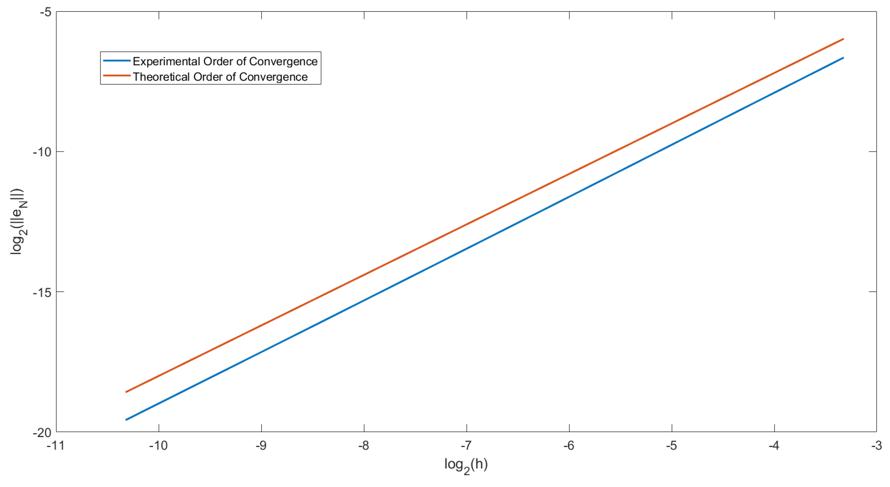
In Figure 1, we have plotted the order of convergence for Example 1. From Equation (24) we have, with $h=1/N$,

$$\left({log}_2\left|\right|e_N\left|\right|\right)\le \left({log}_{2}C\right)+\left({log}_2{N}^{-(1+\alpha )}\right)\le \left({log}_{2}C\right)+\left(1+\alpha \right)\left({log}_{2}h\right).$$

Figure 1. Graph showing the experimental order of convergence (EOC) at T = 2 in Example 1 with $\alpha =0.8$.

Let $y=\left({log}_2\left|\right|e_N\left|\right|\right)$ and let $x=\left({log}_{2}h\right)$. We then plotted a graph for y against x for $h=\frac{1}{5\times 2^l},l=0,1,\dots ,7$. Doing this, we get that the gradient of the graph would equal the EOC. To compare this to the theoretical order of convergence, we have also plotted the straight line $y=(1+\alpha )x$. For Figure 1 we choose $\alpha =0.8$. We can observe that the two lines drawn are parallel. Therefore we can conclude that the order of convergence of this predictor-corrector method is $O\left(h^{1+\alpha }\right)$.

Example 2.

Consider the following nonlinear fractional differential equation, with $\alpha ,\beta \in (0,1)$ and $a=1$,

$$\left\{\begin{array}{c}{{}_{CH}D}_{a,t}^{\alpha }y\left(t\right)=f(t,y),1\le a<t\le T,\hfill \\ y\left(a\right)=0,\hfill \end{array}\right.$$

(25)

where

$$f(t,y)=\frac{\Gamma (1+\beta )}{\Gamma (1+\beta -\alpha )}{(logt)}^{\beta -\alpha }+{(logt)}^{2\beta }-y^2.$$

We will be solving Example 2 over the interval $[1,2]$. The exact solution of this equation is $y={(log\frac{t}{a})}^{\beta }$ and ${{}_{CH}D}_{a,t}^{\alpha }y\left(t\right)=\frac{\Gamma (1+\beta )}{\Gamma (1+\beta -\alpha )}{(logt)}^{\beta -\alpha }$. This implies that the regularity of ${{}_{CH}D}_{a,t}^{\alpha }y\left(t\right)$ behaves as ${(logt)}^{\beta -\alpha }$. This means that ${{}_{CH}D}_{a,t}^{\alpha }y\left(t\right)$ satisfies Assumption 1. We will be using the same graded mesh as in Example 1. Therefore, we have by Theorem 3, with $\sigma =\beta -\alpha$,

$$\left|\right|e_N\left|\right|:=\underset{0\le j\le N}{max}|y\left(t_j\right)-y_j|\le \left\{\begin{array}{c}C{N}^{-r\beta },\mathrm{if}r<\frac{1+\alpha }{\beta },\hfill \\ C{N}^{-r\beta }logN,\mathrm{if}r=\frac{1+\alpha }{\beta },\hfill \\ C{N}^{-(1+\alpha )},\mathrm{if}r>\frac{1+\alpha }{\beta }.\hfill \end{array}\right.$$

(26)

In Table 2, Table 3 and Table 4 we can see the EOC for the predictor-corrector method with varying values of $\alpha$ and with r values at $r=1$ and $r=\frac{1+\alpha }{\beta }$. With a fixed $\beta =0.9$ we have obtain the EOC and maximum absolute error for increasing values of N. By doing so we can see that the EOC are almost $O\left(N^{-r\beta }\right)=0.9$ when $r=1$ and the EOC are almost $O\left(N^{-(1+\alpha )}\right)=1+\alpha$ when $r=\frac{1+\alpha }{\beta }$.

Table 2. Table showing the maximum absolute error and EOC for solving (25) using the predictor-corrector method for $\alpha =0.4,\beta =0.9$.

N	$\mathit{r}=1$	EOC	$\mathit{r}=\frac{1+\mathit{\alpha }}{\mathit{\beta }}$	EOC
10	1.100 × 10${}^{-2}$		1.858 × 10${}^{-2}$
20	5.635 × 10${}^{-3}$	0.965	6.141 × 10${}^{-3}$	1.598
40	3.177 × 10${}^{-3}$	0.827	2.048 × 10${}^{-3}$	1.584
80	1.737 × 10${}^{-3}$	0.871	7.009 × 10${}^{-4}$	1.547
160	9.380 × 10${}^{-4}$	0.889	2.457 × 10${}^{-4}$	1.512
320	5.043 × 10${}^{-4}$	0.895	8.780 × 10${}^{-5}$	1.485
640	2.706 × 10${}^{-4}$	0.898	3.184 × 10${}^{-5}$	1.464
1280	1.451 × 10${}^{-4}$	0.899	1.167 × 10${}^{-5}$	1.448

Table 3. Table showing the maximum absolute error and EOC for solving (25) using the predictor-corrector scheme for $\alpha =0.6,\beta =0.9$.

N	$\mathit{r}=1$	EOC	$\mathit{r}=\frac{1+\mathit{\alpha }}{\mathit{\beta }}$	EOC
10	2.151 × 10${}^{-2}$		6.370 × 10${}^{-3}$
20	1.193 × 10${}^{-2}$	0.851	1.922 × 10${}^{-3}$	1.728
40	6.468 × 10${}^{-3}$	0.883	5.954 × 10${}^{-4}$	1.691
80	3.480 × 10${}^{-3}$	0.894	1.888 × 10${}^{-4}$	1.657
160	1.868 × 10${}^{-3}$	0.898	6.083 × 10${}^{-5}$	1.634
320	1.001 × 10${}^{-3}$	0.899	1.980 × 10${}^{-5}$	1.620
640	5.368 × 10${}^{-4}$	0.900	6.482 × 10${}^{-6}$	1.611
1280	2.877 × 10${}^{-4}$	0.900	2.130 × 10${}^{-6}$	1.605

Table 4. Table showing the maximum absolute error and EOC for solving (25) using the predictor-corrector method for $\alpha =0.8,\beta =0.9$.

N	$\mathit{r}=1$	EOC	$\mathit{r}=\frac{1+\mathit{\alpha }}{\mathit{\beta }}$	EOC
10	3.536 × 10${}^{-2}$		4.523 × 10${}^{-3}$
20	1.916 × 10${}^{-2}$	0.884	1.299 × 10${}^{-3}$	1.800
40	1.030 × 10${}^{-2}$	0.895	3.731 × 10${}^{-4}$	1.800
80	5.528 × 10${}^{-3}$	0.898	1.071 × 10${}^{-4}$	1.800
160	2.963 × 10${}^{-3}$	0.900	3.077 × 10${}^{-5}$	1.800
320	1.588 × 10${}^{-3}$	0.900	8.836 × 10${}^{-6}$	1.800
640	8.510 × 10${}^{-4}$	0.900	2.537 × 10${}^{-6}$	1.800
1280	4.561 × 10${}^{-4}$	0.900	7.287 × 10${}^{-7}$	1.800

When $r=1$, we are using a uniform mesh and we can see that the EOC obtained is the same as those obtained by Gohar et al. [13]. Comparing these to the results of the graded mesh when $r=\frac{1+\alpha }{\beta }$ we can see that a higher EOC has been obtained and an optimal order of convergence is recovered.

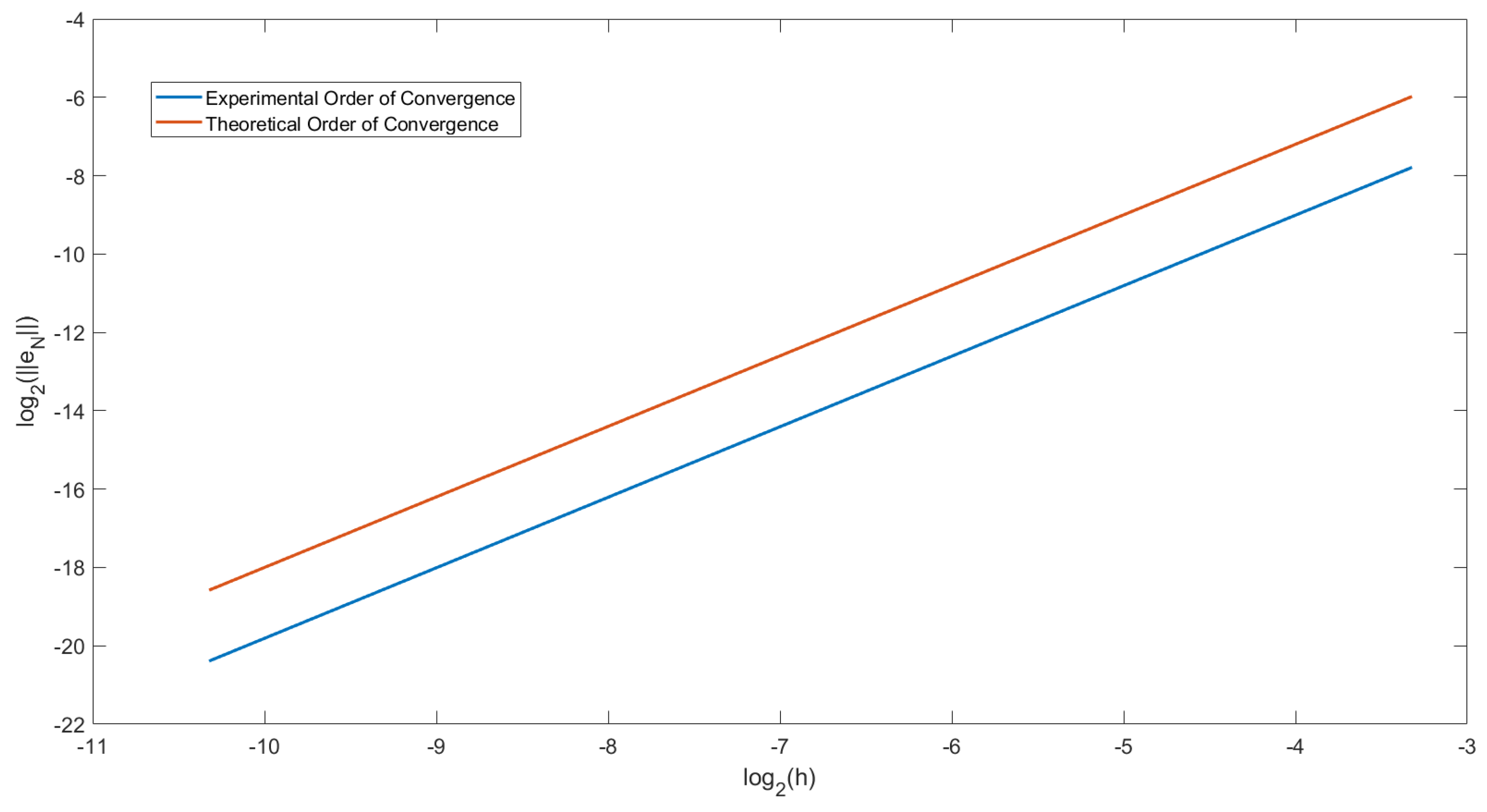
In Figure 2, we have plotted the order of convergence for Example 2 when $r=\frac{1+\alpha }{\beta }$ and $\alpha =0.8$. This plot is the same as for Figure 1. We have also plotted the straight line $y=(1+\alpha )x$. We can observe that the two lines drawn are parallel. Therefore we can conclude that the order of convergence of this predictor-corrector method is $O\left(h^{1+\alpha }\right)$.

Figure 2. Graph showing the experimental order of convergence (EOC) at T = 2 in Example 2 with $\alpha =0.8$ and $r=\frac{1+\alpha }{\beta }$.

Example 3.

Consider the following nonlinear fractional differential equation, with $\alpha ,\beta \in (0,1)$ and $a=1$,

$$\left\{\begin{array}{c}{{}_{CH}D}_{a,t}^{\alpha }y\left(t\right)+y\left(t\right)=0,1\le a<t\le T,\hfill \\ y\left(a\right)=1,\hfill \end{array}\right.$$

(27)

The exact solution of this FODE is $y\left(t\right)=E_{\alpha ,1}\left(-{(logt)}^{\alpha }\right)$. Therefore ${{}_{CH}D}_{a,t}^{\alpha }y\left(t\right)=-E_{\alpha ,1}\left(-{(logt)}^{\alpha }\right)$, where $E_{\alpha ,\gamma }\left(z\right)$ is defined as the Mittag–Leffler function

$$E_{\alpha ,\gamma }\left(z\right)=\sum _{k=0}^{\infty }\frac{z^k}{\Gamma (\alpha k+\gamma )},\alpha ,\gamma >0.$$

Therefore

$${{}_{CH}D}_{a,t}^{\alpha }y\left(t\right)=-\sum _{k=0}^{\infty }\frac{{\left(-logt\right)}^{\alpha k}}{\Gamma (\alpha k+\gamma )}=-1-\frac{{\left(-logt\right)}^{\alpha }}{\Gamma (\alpha +1)}-\frac{{\left(logt\right)}^{2\alpha }}{\Gamma (\alpha +1)}-\dots ,\alpha >0.$$

This shows that ${{}_{CH}D}_{a,t}^{\alpha }y\left(t\right)$ behaves as $c+c{\left(logt\right)}^{\alpha }.$ This means that ${{}_{CH}D}_{a,t}^{\alpha }y\left(t\right)$ satisfies Assumption 1. Therefore, with $\sigma =\alpha$, we have by Theorem 3,

$$\left|\right|e_N\left|\right|:=\underset{0\le j\le N}{max}|y\left(t_j\right)-y_j|\le \left\{\begin{array}{c}C{N}^{-r\left(2\alpha \right)},\mathrm{if}r<\frac{1+\alpha }{2\alpha },\hfill \\ C{N}^{-r\left(2\alpha \right)}logN,\mathrm{if}r=\frac{1+\alpha }{2\alpha },\hfill \\ C{N}^{-(1+\alpha )},\mathrm{if}r>\frac{1+\alpha }{2\alpha }.\hfill \end{array}\right.$$

(28)

We will be solving this equation over the same graded mesh as in Example 1 with varying r values. In Table 5, Table 6 and Table 7, we have calculated the EOC and maximum absolute error with respect to increasing N values and with r values at $r=1$ and $r=\frac{1+\alpha }{2\alpha }$. The experimental orders of convergence are shown to be almost $O\left(N^{r\left(2\alpha \right)}\right)$ if we choose $r=1$ and almost $O\left(N^{r(1+\alpha )}\right)$ if we choose $r=\frac{(1+\alpha )}{2\alpha }$. Once again it is shown when we use a graded mesh at the optimal r value, we get a higher order of convergence to that obtained by the uniform mesh at $r=1$.

Table 5. Table showing the maximum absolute error and EOC for solving (27) using the predictor-corrector method for $\alpha =0.4$.

N	$\mathit{r}=1$	EOC	$\mathit{r}=\frac{1+\mathit{\alpha }}{2\mathit{\alpha }}$	EOC
10	9.399 × 10${}^{-3}$		3.677 × 10${}^{-3}$
20	2.049 × 10${}^{-3}$	2.197	1.234 × 10${}^{-3}$	1.575
40	4.752 × 10${}^{-4}$	2.108	4.687 × 10${}^{-4}$	1.397
80	1.000 × 10${}^{-3}$	−1.074	2.116 × 10${}^{-4}$	1.147
160	9.226 × 10${}^{-4}$	0.116	8.834 × 10${}^{-5}$	1.260
320	6.885 × 10${}^{-4}$	0.422	3.542 × 10${}^{-5}$	1.319
640	4.670 × 10${}^{-4}$	0.560	1.388 × 10${}^{-5}$	1.352
1280	3.002 × 10${}^{-4}$	0.637	5.367 × 10${}^{-6}$	1.371

Table 6. Table showing the maximum absolute error and EOC for solving (27) using the predictor-corrector method for $\alpha =0.6$.

N	$\mathit{r}=1$	EOC	$\mathit{r}=\frac{1+\mathit{\alpha }}{2\mathit{\alpha }}$	EOC
10	6.864 × 10${}^{-4}$		1.512 × 10${}^{-3}$
20	9.020 × 10${}^{-4}$	−0.394	4.756 × 10${}^{-4}$	1.669
40	5.967 × 10${}^{-4}$	0.645	1.766 × 10${}^{-4}$	1.429
80	3.767 × 10${}^{-4}$	0.914	6.423 × 10${}^{-5}$	1.459
160	1.495 × 10${}^{-4}$	1.034	2.233 × 10${}^{-5}$	1.524
320	6.982 × 10${}^{-5}$	1.098	7.587 × 10${}^{-6}$	1.558
640	3.177 × 10${}^{-5}$	1.136	2.545 × 10${}^{-6}$	1.576
1280	1.423 × 10${}^{-5}$	1.159	8.473 × 10${}^{-7}$	1.586

Table 7. Table showing the maximum absolute error and EOC for solving (27) using the predictor-corrector method for $\alpha =0.8$.

N	$\mathit{r}=1$	EOC	$\mathit{r}=\frac{1+\mathit{\alpha }}{2\mathit{\alpha }}$	EOC
10	4.175 × 10${}^{-4}$		6.100 × 10${}^{-4}$
20	1.700 × 10${}^{-4}$	1.297	1.717 × 10${}^{-4}$	1.829
40	7.021 × 10${}^{-5}$	1.275	4.972 × 10${}^{-5}$	1.788
80	2.589 × 10${}^{-5}$	1.439	1.459 × 10${}^{-5}$	1.769
160	9.062 × 10${}^{-6}$	1.514	4.308 × 10${}^{-6}$	1.760
320	3.089 × 10${}^{-6}$	1.553	1.274 × 10${}^{-6}$	1.758
640	1.038 × 10${}^{-6}$	1.574	3.766 × 10${}^{-7}$	1.758
1280	3.459 × 10${}^{-7}$	1.585	1.111 × 10${}^{-7}$	1.760

In Figure 3, we have plotted the order of convergence for Example 3 when $r=\frac{1+\alpha }{\beta }$ and $\alpha =0.8$. This plot is the same as for Figure 1. We have also plotted the straight line $y=(1+\alpha )x$. We can observe that the two lines drawn are parallel. Therefore we can conclude that the order of convergence of this predictor-corrector method is $O\left(h^{1+\alpha }\right)$ for choosing the suitable graded mesh ratio r.

Figure 3. Graph showing the experimental order of convergence (EOC) at T = 2 in Example 3 with $\alpha =0.8$ and $r=\frac{1+\alpha }{2\alpha }$.

Example 4.

In this example we will be applying the rectangular and trapezoidal methods for solving (27). Let N be a positive integer and let $log{t}_j=loga+\left(log{t}_N-loga\right)\frac{j(j+1)}{N(N+1)}$ be the graded mesh on the interval $[loga,logT]$ for $j=0,1,2,\dots ,N$. We will be using $a=1$ and $T=2$.

In Table 8, we have calculated the EOC and maximum absolute error with respect to increasing N values and with $\alpha =0.2,0.4,0.6$ for the rectangular method. By once again using the fact that $\sigma =\alpha$ and applying Theorem 4 we can say

$$\underset{0\le j\le N}{max}|y\left(t_j\right)-y_j|\le \left\{\begin{array}{c}C{N}^{-4\alpha },\mathrm{if}0<4\alpha <1,\hfill \\ C{N}^{-4\alpha }log\left(N\right),\mathrm{if}4\alpha =1,\hfill \\ C{N}^{-1},\mathrm{if}4\alpha >1.\hfill \end{array}\right.$$

Table 8. Table showing the maximum absolute error and EOC for solving (27) using the rectangular method on a graded mesh.

N	$\mathit{\alpha }=0.2$	EOC	$\mathit{\alpha }=0.4$	EOC	$\mathit{\alpha }=0.6$	EOC
40	7.919 × 10${}^{-2}$		8.348 × 10${}^{-3}$		2.852 × 10${}^{-3}$
80	4.843 × 10${}^{-2}$	0.710	2.869 × 10${}^{-3}$	1.141	1.404 × 10${}^{-3}$	1.023
160	2.921 × 10${}^{-2}$	0.730	9.688 × 10${}^{-4}$	1.166	6.951 × 10${}^{-4}$	1.014
320	1.742 × 10${}^{-2}$	0.745	3.239 × 10${}^{-4}$	1.181	3.454 × 10${}^{-4}$	1.009
640	1.030 × 10${}^{-2}$	0.758	1.491 × 10${}^{-4}$	1.119	1.720 × 10${}^{-4}$	1.006
1280	6.053 × 10${}^{-3}$	0.767	7.336 × 10${}^{-5}$	1.023	8.577 × 10${}^{-5}$	1.004

The experimental orders of convergence are shown to be almost $O\left(N^{-4\alpha }\right)$ if we choose $\alpha <0.25$ and almost $O\left(N^{-1}\right)$ if we choose $\alpha \ge 0.25$. This confirms the theoretical error estimates calculated in Section 4. In Table 9, we have used the same method to solve (27) but using the uniform mesh. This shows how a larger EOC is achieved when using non-uniform mesh over a uniform mesh.

Table 9. Table showing the maximum absolute error and EOC for solving (27) using the rectangular method on a uniform mesh.

N	$\mathit{\alpha }=0.2$	EOC	$\mathit{\alpha }=0.4$	EOC	$\mathit{\alpha }=0.6$	EOC
40	1.734 × 10${}^{-1}$		4.650 × 10${}^{-2}$		9.971 × 10${}^{-3}$
80	1.375 × 10${}^{-1}$	0.335	2.795 × 10${}^{-2}$	0.735	4.475 × 10${}^{-3}$	1.156
160	1.085 × 10${}^{-1}$	0.342	1.661 × 10${}^{-2}$	0.751	1.986 × 10${}^{-3}$	1.172
320	8.519 × 10${}^{-2}$	0.348	9.793 × 10${}^{-3}$	0.762	8.750 × 10${}^{-4}$	1.182
640	6.667 × 10${}^{-2}$	0.354	5.737 × 10${}^{-3}$	0.771	3.839 × 10${}^{-4}$	1.189
1280	5.199 × 10${}^{-2}$	0.359	3.345 × 10${}^{-3}$	0.778	1.728 × 10${}^{-4}$	1.152

In Table 10, we have calculated the EOC and maximum absolute error with respect to increasing N values and with $\alpha =0.2,0.4,0.6$ for the trapezoidal method. By once again using the fact that $\sigma =\alpha$ and applying Theorem 4 we can say

$$\underset{0\le j\le N}{max}|y\left(t_j\right)-y_j|\le \left\{\begin{array}{c}C{N}^{-4\alpha },\mathrm{if}0<4\alpha <2,\hfill \\ C{N}^{-4\alpha }log\left(N\right),\mathrm{if}4\alpha =2,\hfill \\ C{N}^{-2},\mathrm{if}4\alpha >2.\hfill \end{array}\right.$$

Table 10. Table showing the maximum absolute error and EOC for solving (27) using the trapezoidal method on a graded mesh.

N	$\mathit{\alpha }=0.2$	EOC	$\mathit{\alpha }=0.4$	EOC	$\mathit{\alpha }=0.6$	EOC
40	8.193 × 10${}^{-3}$		1.266 × 10${}^{-3}$		9.466 × 10${}^{-5}$
80	5.211 × 10${}^{-3}$	0.653	4.391 × 10${}^{-4}$	1.527	1.832 × 10${}^{-5}$	2.370
160	3.241 × 10${}^{-3}$	0.685	1.491 × 10${}^{-4}$	1.559	3.506 × 10${}^{-6}$	2.385
320	1.981 × 10${}^{-3}$	0.711	5.000 × 10${}^{-5}$	1.577	6.675 × 10${}^{-7}$	2.393
640	1.193 × 10${}^{-3}$	0.731	1.664 × 10${}^{-5}$	1.587	1.321 × 10${}^{-7}$	2.338
1280	7.110 × 10${}^{-4}$	0.747	5.517 × 10${}^{-6}$	1.593	3.300 × 10${}^{-8}$	2.003

The experimental orders of convergence are shown to be almost $O\left(N^{-4\alpha }\right)$ if we choose $\alpha <0.5$ and almost $O\left(N^{-2}\right)$ if we choose $\alpha \ge 0.5$. This confirms the theoretical error estimates calculated in Section 4. In Table 11, we have used the same method to solve (27) but using the uniform mesh. This shows how a larger EOC is achieved when using graded mesh over a uniform mesh.

Table 11. Table showing the maximum absolute error and EOC for solving (27) using the trapezoidal method on a uniform mesh.

N	$\mathit{\alpha }=0.2$	EOC	$\mathit{\alpha }=0.4$	EOC	$\mathit{\alpha }=0.6$	EOC
40	1.640 × 10${}^{-2}$		6.803 × 10${}^{-3}$		7.617 × 10${}^{-4}$
80	1.341 × 10${}^{-2}$	0.291	4.150 × 10${}^{-3}$	0.713	2.106 × 10${}^{-4}$	1.854
160	1.087 × 10${}^{-2}$	0.302	2.494 × 10${}^{-3}$	0.735	5.850 × 10${}^{-5}$	1.848
320	8.754 × 10${}^{-3}$	0.313	1.482 × 10${}^{-3}$	0.751	1.632 × 10${}^{-5}$	1.842
640	7.001 × 10${}^{-3}$	0.322	8.733 × 10${}^{-4}$	0.763	4.568 × 10${}^{-6}$	1.837
1280	5.567 × 10${}^{-3}$	0.331	5.115 × 10${}^{-4}$	0.719	1.283 × 10${}^{-6}$	1.832

5. Conclusions

In this paper we propose several numerical methods for solving Caputo–Hadamard fractional differential equations with graded and non-uniform meshes. We first introduce a predictor-corrector method and calculate the convergence and error estimates over a graded mesh so to show that the optimal convergence orders can be recovered when the solutions are not sufficiently smooth. We then introduce the error estimates on the fractional rectangle and fractional trapezoidal methods with some non-uniform meshes. Finally, we consider several numerical simulations to support the theoretical results made for the above methods on the convergence orders and error estimates.

References

1. Diethelm, K. The Analysis of Fractional Differential Equations; Lecture Notes in Mathematics; Springer: Berlin/Heidelberg, Germany, 2010. [Google Scholar]
2. Kilbas, A.A.; Srivastava, H.M.; Trujillo, J.J. Theory and Applications of Fractional Differential Equations; North-Holland Mathematics Studies; Elsevier: Amsterdam, The Netherlands, 2006; Volume 204. [Google Scholar]
3. Oldman, B.K.; Spanier, J. The Fractional Calculus; Academic Press: New York, NY, USA, 1974. [Google Scholar]
4. Podlubny, I. Fractional Differential Equations; Math, Science and Engineering; Academic Press: San Diego, CA, USA, 1999. [Google Scholar]
5. Adjabi, Y.; Jarad, F.; Baleanu, D.; Abdeljawad, T. On Cauchy problems with Caputo Hadamard fractional derivatives. J. Comput. Anal. Appl. 2016, 21, 661–681. [Google Scholar]
6. Garra, R.; Mainardi, F.; Spada, G. A generalization of the Lomnitz logarithmic creep law via Hadamard fractional calculus. Chaos Solitons Fractals 2017, 102, 333–338. [Google Scholar] [CrossRef] [Green Version]
7. Gohar, M.; Li, C.; Yin, C. On Caputo Hadamard fractional differential equations. Int. J. Comput. Math. 2020, 97, 1459–1483. [Google Scholar] [CrossRef]
8. Jarad, F.; Abdeljawad, T.; Baleanu, D. Caputo-type modification of the Hadamard fractional derivatives. Adv. Differ. Equ. 2012, 2012, 142. [Google Scholar] [CrossRef] [Green Version]
9. Kilbas, A.A. Hadamard-type fractional calculus. J. Korean Math. Soc. 2001, 38, 1191–1204. [Google Scholar]
10. Li, C.; Cai, M. Theory and Numerical Approximations of Fractional Integrals and Derivatives; SIAM: Philadelphia, PA, USA, 2019. [Google Scholar]
11. Ma, L. On the kinetics of Hadamard-type fractional differential systems. Fract. Calc. Appl. Anal. 2020, 23, 553–570. [Google Scholar] [CrossRef]
12. Hadamard, J. Essai sur létude des fonctions donnes par leur developpment de Taylor. J. Pure Appl. Math. 1892, 4, 101–186. [Google Scholar]
13. Gohar, M.; Li, C.; Li, Z. Finite Difference Methods for Caputo-Hadamard Fractional Differential Equations. Mediterr. J. Math. 2020, 17, 194. [Google Scholar] [CrossRef]
14. Abbas, S.; Benchohra, M.; Hamidi, N.; Henderson, J. Caputo-Hadamard fractional differential equations in Banach spaces. Fract. Calc. Appl. Anal. 2018, 21, 1027–1045. [Google Scholar] [CrossRef]
15. Samei, M.E.; Hedayati, V.; Rezapour, S. Existence results for a fraction hybrid differential inclusion with Caputo–Hadamard type fractional derivative. Adv. Differ. Equ. 2019, 2019, 163. [Google Scholar] [CrossRef]
16. Ardjouni, A. Existence and uniqueness of positive solutions for nonlinear Caputo-Hadamard fractional differential equations. Proyecciones 2021, 40, 139–152. [Google Scholar] [CrossRef]
17. Li, C.; Li, Z.; Wang, Z. Mathematical Analysis and the Local Discontinuous Galerkin Method for Caputo-Hadamard Fractional Partial Differential Equation. J. Sci. Comput. 2020, 85, 41. [Google Scholar] [CrossRef]
18. Liu, Y.; Roberts, J.; Yan, Y. Detailed error analysis for a fractional Adams method with graded meshes. Numer. Algorithms 2018, 78, 1195–1216. [Google Scholar] [CrossRef] [Green Version]
19. Liu, Y.; Roberts, J.; Yan, Y. A note on finite difference methods for nonlinear fractional differential equations with non-uniform meshes. Int. J. Comput. Math. 2018, 95, 1151–1169. [Google Scholar] [CrossRef]
20. Li, C.; Yi, Q.; Chen, A. Finite difference methods with non-uniform meshes for nonlinear fractional differential equations. J. Comput. Phys. 2016, 316, 614–631. [Google Scholar] [CrossRef]
21. Diethelm, K. Generalized compound quadrature formulae for finite-part integrals. IMA J. Numer. Anal. 1997, 17, 479–493. [Google Scholar] [CrossRef]
22. Zhang, Y.; Sun, Z.; Liao, H. Finite difference methods for the time fractional diffusion equation on non-uniform meshes. Int. J. Comput. Math. 2014, 265, 195–210. [Google Scholar] [CrossRef]
23. Stynes, M. Too much regularity may force too much uniqueness. Fract. Calc. Appl. Anal. 2016, 19, 1554–1562. [Google Scholar] [CrossRef] [Green Version]
24. Stynes, M.; Oriordan, E.; Gracia, J.L. Error analysis of a finite difference method on graded meshes for a time-fractional diffusion equation. SIAM J. Numer. Anal. 2017, 55, 1057–1079. [Google Scholar] [CrossRef]
25. Lubich, C. Runge-Kutta theory for Volterra and Abel integral equations of the second kind. Math. Comput. 1983, 41, 87–102. [Google Scholar] [CrossRef]
Publisher’s Note: MDPI stays neutral with regard to jurisdictional claims in published maps and institutional affiliations.
Article Metrics
Citations
Article Access Statistics
Multiple requests from the same IP address are counted as one view.