Abstract
In this paper, we provide a mathematical and statistical methodology using heteroscedastic estimation to achieve the aim of building a more precise mathematical model for complex financial data. Considering a general regression model with explanatory variables (the expected value model form) and the error term (including heteroscedasticity), the optimal expected value and heteroscedastic model forms are investigated by linear, nonlinear, curvilinear, and composition function forms, using the minimum mean-squared error criterion to show the precision of the methodology. After combining the two optimal models, the fitted values of the financial data are more precise than the linear regression model in the literature and also show the fitted model forms in the example of Taiwan stock price index futures that has three cases: (1) before COVID-19, (2) during COVID-19, and (3) the entire observation time period. The fitted mathematical models can apparently show how COVID-19 affects the return rates of Taiwan stock price index futures. Furthermore, the fitted heteroscedastic models also show how COVID-19 influences the fluctuations of the return rates of Taiwan stock price index futures. This methodology will contribute to the probability of building algorithms for computing and predicting financial data based on mathematical model form outcomes and assist model comparisons after adding new data to a database.
1. Introduction
Complex financial time-series data are difficult to fit using a simple model for the core model in artificial intelligence. If we seek to build a more precise model, a simple model form cannot achieve this aim; at the same time, imprecise errors can lead to uncontrollable situations. Researchers have discussed numerous methodologies to solve the discordance between the data regression and the biasedness of the estimation in the traditional regression analysis. For example, data are not independent and identically distributed from a normal distribution. Models are not commonly in linear, quadratic, or cubic form, but in a more complex form. Heteroscedasticity or serial correlation might exist in the data. Those are the three main misspecifications in the regression analysis and the main reasons it is difficult to find a precise model for the data.
The first misspecification that data are not i.i.d. from a normal distribution biases the coefficient estimation in the maximum likelihood estimation (MLE). Golden et al. [1] mentioned this misspecification and viewed it as a kind of model misspecification from the wrong probability distribution. They considered the general and specific probability function to formulate the likelihood function. However, a different conditional probability distribution has its own parameter(s), which is estimated using the characteristic of Yt|Xt = f(Xt) = E(Yt|Xt), a regression model of the expected value. Without considering the distribution assumption in the regression model of the expected value, the method of moments estimators (MME) and the generalized least-square (GLS) estimation are preferred over the MLE method.
The second misspecification is the wrong model form of f(Xt), which is considered a linear model in most of the literature. It should be noted that the residuals of the wrong model form are biased from the errors. Some researchers have considered the cubic function as the regression model and call it the curvilinear regression. Some academic researchers considered the cubic function as the regression model and call it as the curvilinear regression [2], or the quadratic form [3,4]. As researchers intend to generate a high-order polynomial or curvilinear regression to build a more precise model form, an overfitting problem occurs, especially in deep learning [5,6,7,8].
If we only consider the trend model, it is correct to focus on the overfitting problem. If the reason for obtaining the precise model is to predict and to reduce the errors of the model, then should we still follow the trend model up to power-to-three and avoid the overfitting problem? We propose that the complex data pattern should be modeled by using a mathematical model form. Mathematical models can be very complex, especially when using the function composition. Such model can be complex for humans to calculate, but it is a quick calculation for computers. By using computer calculation, we can aim to find the precise mathematical model for complex data and are not limited by the linear model form nor have to deal with the overfitting problems.
The third misspecification is heteroscedasticity and serial correlation. The latter is not discussed in this paper, although the lagged period mainly determines the data prediction and the reasonableness of the linear model assumption. As to the former, heteroscedasticity is one of the main models of this paper and can reduce the errors in the data model. In the literature, there is one common method using the series of the autoregressive (AR) model to solve heteroscedasticity This method is applied to calculate the volatility of financial data—time-series data [9]—such as the ARCH series model, the GARCH model [10,11,12,13], and the EGARCH model [14,15].
To obtain the residuals, the above series of AR models depend on the linear regression model form and normal distribution assumption, without considering whether or not the data characteristics satisfy those assumptions. Even though the fitted linear regression model and the prediction seem sound, addressing the second misspecification can solve the problem that the residuals are biased from the errors. The correction of the error term is for the precise fittings of the expected value model and the heteroscedastic model so that we can find values of the dependent variables that contain a low error.
Data analysts face these three misspecifications simultaneously, so we attempt to find the heteroscedastic model by following the approach of the expected value model and combine them as a mathematical model, which will provide relative precision compared to others. Because the errors are small enough in the mathematical model that we can find out, the model is the optimal one for the complex financial data. A few pieces of literature discuss this topic and the method for this kind of combination, but this is a very important key for the core model in programming.
The example that we employed in this paper is Taiwan stock price index futures, which is the financial derivate of the Taiwan stock price index and has the contract characteristic. Another financial derivate is MSCI Morgan Taiwan index futures commonly invested by Taiwan investors. The selected period includes the COVID-19 pandemic. The futures characteristics lead to nonlinear and more complex function behavior in the closing prices of Taiwan stock price futures. The example can show how the approach works to obtain the mathematical model equations, which can be compared to other models and used to find the change of Taiwan stock price index futures before and during COVID-19.
As our primary contribution, this paper provides an approach to heteroscedasticity and model precision to solve the problem of misspecifications in the regression model. This kind of approach can build a precise mathematical model of the data, which can be used in artificial intelligence algorithms to avoid the problems associated with the criterion of accuracy indicators in order to visualize the mathematical form and further compare the model forms while the new data are recorded in a database. The empirical results of the example show that the COVID-19 pandemic affects the expected value model and heteroscedastic model forms of Taiwan stock price index futures. The models of the expected value and heteroscedasticity can be combined and reveal the highest precision with the minimal mean-squared errors of the mathematical models.
The structure of this paper is as follows. Section 2 describes the methodology of the models of the expected value and heteroscedasticity, and the nonlinear model forms selection criteria and the optimal models for financial time-series data. Section 3 describes the data source of observations including Taiwan stock price index futures, MSCI Morgan Taiwan index futures, and Taiwan stock price index. Section 4 shows the results of the estimation models of the expected value before and during COVID-19 and the results of the heteroscedastic estimation models before and during COVID-19. Section 5 concludes the paper.
2. Methodology
To address our research aim of finding the mathematical model of complex financial data, we build the function f:{X} → {Y}, where X = (X1,t, X2,t,⋯, Xp,t) ∈ ℜ and Y = (Yt) ∈ ℜ. The estimated model is:
where p = 1, 2, ⋯, p, t = 1, 2,⋯, T and εt is the error term. The fitting correct form of f(•) is difficult and induces the mistake of a wrong model form, which is labeled as δt. Equation (1) becomes:
Sometimes, the mistake from fitting the wrong model form might be a function of X, that is δt = δ(X1,t, X2,t,⋯, Xp,t). In this situation, where the residuals include δt + εt after the estimation, the biasness of the estimator always exists in heteroscedasticity, as does the bias measure of the mean-squared error. We need to find the relatively precise mathematical model of financial data to let δt be small enough so that fw(•) approximates f(•), which achieves the aim of this paper.
2.1. Model of the Expected Value
We now illustrate the concept presented in this subsection in the context of the estimation of the expected value. In that case, we can confer the right interpretation to let fw(•) → f(•). The regression analysis always depends on the linear model form, which is used to estimate the model of complex financial data as fw(•). More precisely, this is why researchers always use the series of autoregressive models, such as the ARCH model or GARCH model, to find the volatility of financial data. We can let fw(•) be linear, nonlinear, or curvilinear model forms of the expected values of financial data. Suppose a nonlinear model including the linear model is:
where Zi(•) is a nonlinear model form from 37 mathematical functions (see Appendix A), βi is the coefficients of Zi(•), and τt is the error term of (3), different from εt. τt follows a specific probability distribution, P(τt), and satisfies E(τt) = E(Xi,t τt) = 0, i = 1, 2,⋯, p. The optimal Zi(•) is determined by the maximum correlation coefficient after an explanatory variable is transferred by 37 functions, that is max r(Yt, Z(Xi,t)). However, f(•) might be a complex model form and cannot be formatted by a nonlinear model. We let τt approach εt, implying the mistake of the model form for the expected value is as small as possible. The curvilinear regression is a good estimate for this paper. Because the curvilinear regression is based on a Taylor expansion that expands from a point value of an explanatory variable, the fitted values of (3) can be a new explanatory variable in the curvilinear regression model and the average of the fitted values of (3) can be the average where the explanatory variable is expanded. Therefore, (3) can be formed as:
Let be the fitted value of (3) at time t and H(•) is the general curvilinear regression model form with higher power labelled by m. There are five model forms of V(•) used to find the optimal curvilinear regression model form, and these are given as follows:
where the optimal function form of V(•) is from the estimations of (5)–(9), where M is determined by the maximum determination coefficient, R2. βm is the coefficient of V(•) and m corresponds to the power from zero to M (up to 40). To determine the optimal value of M, we record the mean-squared error after running one additional explanatory variable with the power m + 1. The optimal M is determined by the minimal mean-squared error from 40 mean-squared errors.
The approach for estimating the expected values is a type of two-stage generalized least-square (GLS) estimation. The original two-stage least square estimation is based on the instrument variables (IV) at the first stage and then uses the instrument variable as the explanatory variable to run an OLS estimation. In this paper, we adapt a similar estimation method but use the fitted values of (3) as the explanatory variable to run (4), instead of building the instrument variable.
We have tried to solve the misspecification of the model for the expected value—to reduce the effect of δt in the residuals as much as possible. Because the financial data have complex time-series characteristics, the building model of the Taiwan futures index and the explanatory variables should be investigated by the above estimations where the determination of the optimal one should follow some criterions after the estimations of the expected value.
2.2. Model of Heteroscedasticity
However, the residuals might/might not have heteroscedasticity and serial correlation simultaneously. As we run the regression on the data, there is no information to know if the data has heteroscedasticity and serial correlation. This is why, after the linear regression model is estimated, heteroscedastic tests are used to test the residuals. The most common residual setting is the squared errors as the dependent variable, such as the White test [16], Goldfeld–Quandt test [17], Breusch–Pagan test [18], and Cook–Weisberg test [19]. Regarding the selection of explanatory variables in the heteroscedastic tests, there might be the original explanatory variables or other variables that do not occur in the linear model of the expected value.
Different from the above tests, Glejser [20] chose the absolute values of the residuals as the dependent variable and then tested heteroscedasticity. The squared residuals or the absolute values of the residuals can be used for the heteroscedastic tests because heteroscedasticity is the conditional variances change with the values of the specific explanatory variables, Var(Y|X) = [σ(X)]2 or Var(Y|X) = σ2 ψ(X). However, the absolute value function is superior to the squared value function of the residuals in this paper. This is because we cannot keep the root of the fitted values from the squared residual setting positive, building the combination of the models of the expected value and heteroscedasticity. Thus, we consider the model of heteroscedasticity as:
where is the residual at time t, is the error term of (10) at time t, and G(•) is a regression model that is the optimal one from the five mathematical functions after estimation (see Equations (11)–(15)). Except for (11)–(15), G(•) also fitted the pure linear, nonlinear, and curvilinear models in the forms of (5)–(9).
Equations (11) and (12) are the curvilinear regression expanded from the fitted values of the linear and nonlinear regression, respectively. Equations (13) and (14) are types of composite functions where the first step is to obtain the fitted values from the curvilinear regression for each explanatory variable, and the second step is to run linear and nonlinear regressions with the fitted values at the first step as the explanatory variable. The of Equation (13) is the estimated value of (13a). For the nonlinear regression of (14), Zi(•) or Zj(•) are from 37 mathematical functions. Equation (15) is a benchmark model where there is only one constant value: the average of the residuals. The optimal regression model is selected by the criterion of the minimal mean-squared error.
The advantage of (11) and (12) is that, at the first step, the model can display an apparent trend and easily explain the effects of the explanatory variables in the multivariate regression. The curvilinear regression at the second step can show slight fluctuations in the heteroscedastic model. If Equation (11) or (12) were the optimal selection as the model form, it means that the financial data first shows the main effect of the market power (a linear or nonlinear form); meanwhile, data also shows the external effect as a cyclic fluctuation from the market.
Equations (13) and (14) describe that the slight fluctuations are the main effect of the data, so the curvilinear regression is applied at the first step. We regard the fitted values calculated at the first step as the explanatory variable in the second step and then estimate a stable linear or nonlinear trend. The two equations imply that the data mainly exist as adjusted effects of long-term cyclic policies or economic factors. The cyclic effect is involved by repeatedly implementing short-term policies or interventions. Finally, the determination of the optimal heteroscedastic model, (10), depends on the minimum mean-squared error after the estimations of (11)–(15) and the pure linear, nonlinear, curvilinear models. Only as we raise the precision of the model of the expected value will the residuals reveal more explicit regularity to reduce the estimation errors.
The first advantage of adopting this kind of estimation methodology is that we do not need to obey the normal distribution assumption of the regression model when the data’s distribution is unknown. The assumptions of the regression model are always difficult to satisfy with actual situations of the data; the data regularities are hard to estimate. The second advantage is to reduce a great deal of information falling into the residuals. This is caused by fitting a linear model onto the model of the expected value, which will be biased from the error term and will induce the problem of representativeness. Thus, the complex model forms are better than the linear model and suitable for fitting the relatively precise model of (1) with the trend and the slight regularities; meanwhile, the residuals become better represented than those from the linear estimation.
If we had only considered the model of the expected value, the maximal coefficient of determination (R2) or the minimal mean-squared error would have been good criteria for choosing the optimal model form. Now, however, we decompose the residuals as a function of G(•) and try to build a more precise mathematical model of the data, (1), combining Equations (4) and (5). The optimal model of (5) can reduce the unexplainable part in the regression, so the criterion determining the most optimal model form is apparent in order to use the minimal mean-squared error.
2.3. Back to the Expected Value Model with Heteroscedasticity
The error term in (1) can be replaced by the fitted heteroscedastic model, estimated |εt|, with a positive or negative sign that can be assessed by the original signs of the residuals. Thus, the estimated model of (1) can be shown by the combination of the fitted models of the expected value, (4), and heteroscedasticity, (10). If the original residual () at time t has a positive sign, then the estimated financial data will be:
where is the fitted value of the financial data at time t after model combination, is the fitted value of (4) at time t, and is the fitted value of (10) at time t. If the original residual () at time t has a negative sign, then the estimated financial data will be:
The previous regression analysis views the error term as a disappearance after the estimation that is . The error term in this paper can be fitted by the heteroscedastic model, so becomes to achieve the aim of building a precise model.
The sign of determines that the will be added in or deducted due to . Because is the estimator of , shows as . A positive/negative leads with a positive/negative sign to be /. Due to the estimation model of the expected value, adding the variance heterogeneity estimation model, (16) and (17), will obtain the fitted financial data, with moving up and down determined by the signs of the residuals. This method has the advantage of providing the precision of the comparison between the actual and fitted values. Further, the difference can be calculated from the previous and later-fitted values to obtain volatility. This volatility calculation is not limited to the normal distribution assumption.
3. Samples
The financial dataset is collected from the Taiwan Economic Journal Database (TEJ), including Taiwan stock price index futures (close price after hour), the MSCI Morgen Taiwan index futures, and Taiwan stock price index, from 17 January 2019–29 October 2020. Because the MSCI Morgan Taiwan index futures did not trade after 30 October 2020 (MSCI Morgan Taiwan Index Futures had been indexed and traded in the Singapore Exchange. After the end of the T session on 30 October 2020, MSCI Morgan Taiwan Index Futures was suspended from trading and made dormant thereafter. (https://www.kgieworld.sg/futures/msci-taiwan-index-futures-notice)), only data up to 29 October 2020 is available; there are a total of 431 observations. The daily return rate follows the formula:
and we obtain 430 return rates for each variable. Label Yt is the daily return rate of Taiwan stock price index futures, X2,t is the daily return rate of the MSCI Morgen Taiwan index futures, and X3,t is the daily return rate of the Taiwan stock price index. X1,t = t is the time variable from 1 to 430.
Rt = (ln(Xt) − ln(Xt−1)) × 100%,
In the literature, Albulescu [21,22] included the COVID-19 pandemic data of the World Health Organization in the analysis and discussed the volatility influence of the S&P 500 index in the US financial market. Bakas and Trantafyllou [23] discussed the volatility impact of the COVID-19 pandemic on the rate of return on broad commodity indices, crude oil, and gold prices, using a five-factor VAR model based on a linear regression model with time lags and errors assumed from a normal distribution. However, they did not provide the fitted model form for the data affected by COVID-19. We adopt the above-mentioned methodology to estimate the observations of the three cases separately and try to establish the precise fitted models. The advantage of the fitted models can be compared to see the impact of COVID-19. Suppose that Case 1 is the whole research time period, Case 2 is the case before COVID-19 from 17 January 2019–21 February 2020, in a total of 260 observations, and Case 3 is the case during COVID-19 from 24 February 2020–29 October 2020, in a total of 170 observations.
Table 1 displays the descriptive statistics of Case 1. The medians are larger than the averages for the three variables. Because Taiwan stock price index futures and MSCI Morgan Taiwan index futures are the financial derivatives of the Taiwan stock price index, the standard deviations in the first two columns are larger than the Taiwan stock price index. Regarding the skewness, a negative skewness occurs in the Taiwan stock price index futures and Taiwan stock price index, but the MSCI Morgan Taiwan index futures have positive skewness. The kurtosis coefficients of the three variables are more than three, showing relatively more centralization around the averages.

Table 1.
Descriptive statistics of Case 1.
4. Fitted Models of the Expected Value
Firstly, we estimate the linear regression model as the standard one whose model form is as (19) for Case 1, with the mean-squared error = 0.096555.
Equation (19) shows a simple marginal effect between the Taiwan stock price index futures and each explanatory variable. For the complex financial data, the associations will not be so simple and have relatively large error values. From this study’s methodology, because the expected value estimation has the two fitting stages, the fitted nonlinear models of the expected value in Cases 1 to 3 at the first stage are shown as:
where is the Taiwan stock price index futures in Case 1, is the Taiwan stock price index futures before COVID-19 in Case 2, and is the Taiwan stock price index futures during COVID-19 in Case 3. Comparing (20) and (21), we find that the time variable changes the cycle periodic regularities from the cosine function in (21) to the sine function in (20). All things being equal, the time variable reveals the change of the periodic effect on the Taiwan stock price index futures when the time is from Case 2, pre-COVID-19, to Case 1, where the period covers both pre-COVID-19 and during COVID-19.
Equation (22) shows the mathematical model of Taiwan stock price index futures during COVID-19, and we can find that the COVID-19 event changes the main associations of the time variable on the return rate of Taiwan stock price index futures, revealing a reciprocal inverse effect on Taiwan stock price index futures during COVID-19. The MSCI Morgan Taiwan index futures remain linear and show a similar marginal effect on the return rate of Taiwan stock price index futures, but the Taiwan stock price index enlarges the marginal effect on the return rate of Taiwan stock price index futures.
The fitted models at the second stage are the curvilinear regression models, and the coefficients are shown in Table 2. The optimal M reached 16 for Cases 1 and 3, implying the complex associations after the estimations of (20) and (22). The optimal M is 6 for Case 2, implying that Taiwan stock price index futures before COVID-19 have relatively simple associations. The mean-squared errors of Cases 1–3 have decreased to 0.05653, 0.03793, and 0.08693, respectively, compared to the mean-squared error of (19).
Table 2.
The coefficients of curvilinear regression for the expected value.
This methodology can well estimate the expected value model. Figure 1 shows the fitted values in red and the observations in blue at different horizontal axes displaying the time variable, the MSCI Morgan Taiwan index, and Taiwan stock price index, respectively, in columns 1–3. Each row of Cases 1–3 is displayed from top to bottom.
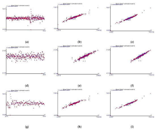
Figure 1.
The actual and fitted values of Cases 1 to 3 on different horizontal axes. The first row is Case 1, the second row is Case 2, and the third row is Case 3. (a,d,g) are based on the horizontal axis as the time variable. (b,e,h) are based on the horizontal axis as the MSCI Morgan Taiwan Index Futures. (c,f,i) are based on the horizontal axis as Taiwan stock price index.
Figure 1 shows the associations of different horizontal axes and Taiwan stock price index futures. Figure 1a,d,g shows the trends of Taiwan stock price index futures in Cases 1–3. Figure 1a is apparently a combination of Figure 1d,g and presents a relatively narrow and stable belt shape trend before COVID-19; Figure 1d also displays a near-belt shape trend. However, Figure 1g shows the converge of volatility for Taiwan stock price index futures during COVID-19.
Another finding is that Taiwan stock price index futures are linearly related to the MSCI Morgan Taiwan index futures in Figure 1b,e,g. Although the correlation coefficients are 94.12%, 94.06%, and 94.50% from the view of the observations, the nonlinear model forms indicate the marginal effects as 0.217, 0.258, and 0.205 (see (19)–(21)), respectively. In fact, the MSCI Morgan Taiwan index futures are not enough to fit Taiwan stock price index futures by a simple linear model form if we intend to input more than one explanatory variable into the model and try to estimate precisely. We also find that the extreme values can be fitted in columns two and three of Figure 1. The graphs show that complex time series financial data fitted by this methodology can simultaneously fit the extreme and centralized observations and decrease the fitting errors.
5. Fitted Heteroscedastic Models
The residuals of Case 1 are estimated, and the model form is (23) where W1 to W3 are estimated by the curvilinear regression. Their coefficients are shown in Table 3. Equation (23) is the optimal model for (11)–(15), with a minimum mean-squared error of 0.02591, and it has a stable and linear model form as the absolute values of the residuals are regressed on each explanatory variable. There are stronger and more complex curvilinear associations between each explanatory variable and the residuals.
Table 3.
Coefficients of curvilinear for each explanatory variable at each Case.
The same can be said for the estimations in Cases 2 and 3. Only considering the observations in Case 2, the fitted heteroscedastic model before COVID-19 is (24), where W1 is a polynomial function expanded at 130.5 with the power to 12, W2 is a polynomial function expanded at 0.08849 with the power to 7, and W3 is a cosine function with the power to 1. After the Wi values are calculated, the absolute values of the residuals for Taiwan stock price index futures before COVID-19 display a nonlinear model form, where W1 is a cubic function but W2 and W3 are trigonometric functions. In Case 3, the fitted heteroscedastic model during COVID-19 is (25), where the transferred explanatory variables, W1~W3, are the polynomial functions with the powers to 6, 16, and 17, respectively. After the Wi values are calculated, the absolute values of the residuals for Taiwan stock price index futures show a linear model form.
The heteroscedastic model of Case 2 is different from the estimated models of Cases 1 and 3, where the fitted heteroscedastic models are (23) and (35), with all Wi showing the polynomial function forms. However, Case 2 consists of the observations before COVID-19, having simpler functions of all Wi than Cases 1 and 3, implying that the influence of COVID-19 changes the associations from simplification to complication (see (23) and (24)). We can find that the observations during COVID-19 dominate the fitted heteroscedastic model as we compare it to the whole period observations. Moreover, the unexplainable parts of Taiwan stock price index futures apparently decrease in Cases 1 to 3 after the estimations of the heteroscedastic model. Table 3 shows the minimum mean-squared errors of Cases 1 to 3 to be 0.02591, 0.0208, and 0.0311, respectively, and the mean-squared errors of all cases in Table 3 are lower than those in Table 2.
This methodology can estimate heteroscedasticity and show the regularities for the absolute values of the residuals. Each column of Figure 2 displays the graphs of the fitted heteroscedastic values at different horizontal axes, labeled by the time variable, the return rates of the MSCI Morgan Taiwan index, and the Taiwan stock price index, respectively. Each row displays an individual case, with three cases in total.
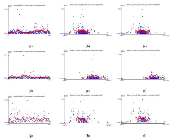
Figure 2.
The fitted residuals result of heteroscedasticity. (a–c) is Case 1; (d–f) is Case 2; and (g–i) is Case 3. See Appendix B with the plots of only the fitted values of the heteroscedastic estimation.
The residuals from the estimation of all observations (Case 1) show that the estimated trend in Figure 2a seems to a be a combination of Figure 2d,g at the time variable horizontal axis. Figure 2d shows that the absolute values of the residuals are flatter as time goes by, in particular, the return rates of Taiwan stock price index futures exceeded 0.2 from 24 June 2019–18 July 2019. Figure 2g shows that the absolute values of the residuals have numerous extreme values, and the observations (in blue) are not centralized. The difference between Figure 2a and Figure 2g is because the data of Figure 2g are only the observations during COVID-19.
Because Case 2 at row two and Case 3 at row three are the case before and during COVID-19, respectively, let us observe Figure 2d–i. Figure 2d–f shows the main regularities for the absolute values of the residuals before COVID-19.
As to the observations, the estimated value of is maximum and around 0.4946%, shown by the highest red point in row 2 in Figure 2, while the return rate of the MSCI Morgan Taiwan Index is around −2.5466% and the return rate of Taiwan stock price index is around −0.3998% on June 28, 2019. The remaining red spots in Figure 2d are spread between 0.0615% and 0.190%. Figure 2e,f shows the main trend in red and some red spots around the area higher than the main trend in red.
Nevertheless, Figure 2g–i distinctly shows that the absolute values of the residuals during COVID-19 have more apparent fluctuations than the values in row 2, and those red points that exceed 0.24%, compared with the upper quartile (Q3 of ) = 0.2344%, are not centralized in a specific time period. Thus, the results of Figure 2d,g prove that the heteroscedastic regularities are also affected by the occurrence of COVID-19.
Fitted Models with the Expected Value and Heteroscedasticity
After adding the estimated heteroscedastic model to replace the error term in the model of the expected value, the fitted values can almost be covered on the observations (blue spots). Regarding row one in Figure 3, the precisely fitted model of Case 1 is as (26) and (27). For instance, Figure 3a shows that the fitted values calculated by (26) and (27) were evaluated more precisely than Figure 1a because the MSE decreases from 0.0565 to 0.0259.
if the original residual () at time t is a positive value, or
if the original residual () at time t is a negative value. As for row two in Figure 3, the precisely fitted model form is as (28) and (29), showing the case before COVID-19.
if the original residual () at time t is a positive value, or
if the original residual () at time t is a negative value. As to row three in Figure 3, the precisely fitted model of Case 3 is formatted as (30) and (31).
if the original residual () at time t is a positive value, or
if the original residual () at time t is a negative value. As for (26)–(31), the coefficients of bm are shown in Table 2 and the Wi, i = 1, 2, 3, are shown in Table 3. The spread of the observations before or during COVID-19 can be formed as a mathematical model and show the precision of the models—that the red spots cover the blue spots with very small distances.
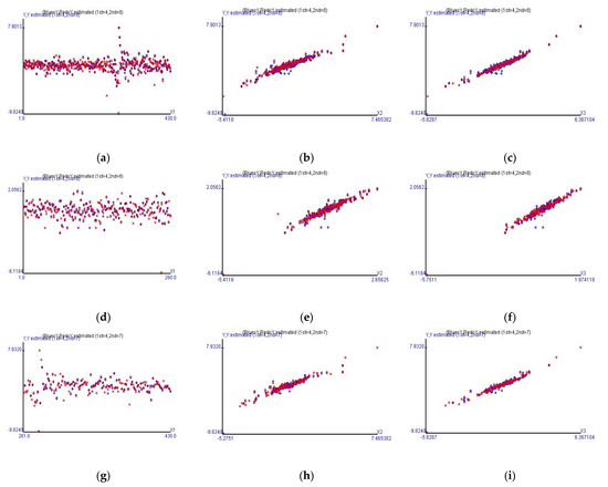
Figure 3.
The actual and fitted values in different cases using the combination of the fitted models of the expected value and heteroscedasticity. (a–c) is Case 1; (d–f) is Case 2; and (g–i) is Case 3.
Figure 3 displays the fitted values calculated by (26)–(31) in different cases. Figure 3b,e,h in the second column shows the linear relationship between Taiwan stock price index futures and the MSCI Taiwan index futures before and during COVID-19; however, the linear relationship is an exceedingly oblate ellipsoid shape, representing the existing possibility of extreme values. The linear relationship between Taiwan stock price index futures and the Taiwan stock price index also shows an exceedingly flat shape of a similar oblate ellipsoid, displayed as red points in Figure 3c,f,i.
6. Conclusions
Comparing Table 2 and Table 3, the mathematical model forms show that Taiwan stock price index futures before COVID-19 have a stable and relatively simple regularity with the MSCI Morgan Taiwan index futures and the Taiwan stock price index. For the data that includes the COVID-19 period—Cases 1 and 3—the regularities of Taiwan stock price index futures become more complex and are fitted by the relatively high-order curvilinear regression so as to obtain precise mathematical models with a minimal mean-squared error value. Even though the mean-squared error values of Cases 1 and 3 are as low as possible, the effect from COVID-19 causes Taiwan stock price index futures to be relatively unstable; however, this unstable regularity can still be driven by the data and is explained by the time variable, the MSCI Morgan Taiwan index futures, and the Taiwan stock price index. It is surprising that the time variable can capture the futures contract characteristic—that is the due date of the cyclic recent month contract—and show the precision of the estimation and the difference for return rates before and during COVID-19.
The different explanatory variables on the horizontal axis are scattered with the fitted values, and the observations show the relationship of the explanatory variable and Taiwan stock price index futures in Figure 1 and Figure 3. Except for the time variable, the MSCI Morgan Taiwan index futures and Taiwan stock price index are linearly related to Taiwan stock price index futures. However, the positive linear relationship is misleading in that the one explanatory variable shown cannot be adequately considered to build a linear regression model. In the cases of this paper, we provide evidence that the highly linear-correlative explanatory variables are good for the linear regression model; however, slight fluctuations can also be fitted, even if the explanatory variable is highly linearly related to Taiwan stock price index futures. The maturity characteristics of the futures contracts, which cause slight fluctuations or volatilities, can also be fitted with the time variable for the expected value estimation. The remaining residuals can be fitted with the explanatory variables following the residual plot concept.
This paper indicates the importance of data for building mathematical models that can further achieve the aim of building a precise mathematical model that can, for example, be the core algorithm of an artificial intelligence system for computing complex financial data. A mathematical model is standard for understanding the precision and accuracy of a data model. Providing a data-driven methodology to find a mathematical model is vital for artificial intelligence as new data are recorded into a database. The previous model form can be compared with the model estimated with new data so as to accentuate the change of the model form as a signal of event occurrences. Thus, this paper contributes to providing a methodology to build a precise model for complex financial data—our data-driven model is different from model settings recognized by researchers, which can be considered. Moreover, the complex financial data can be formatted as a mathematical model chosen from numerous models following the criterion of the minimal MSE. This kind of model increases the precision in order to predict the next step, which was not the aim of this work but could be a future research direction.
This paper shows the associations between Taiwan stock price index futures and explanatory variables and also demonstrates apparent mathematical models to compare COVID-19′s effect on Taiwan stock price index futures. However, this paper has some limitations. For instance, the explanatory variables of the example were chosen by the scenario in which we followed the concept of financial derivatives without considering more variables, such as nonfinancial variables. Moreover, the data characteristics also limited the analysis. Collecting more indicators or indices in a database could allow for choosing explanatory variables via the correlation coefficients of all the explanatory variables we can find. Our results could be utilized as a data-driven methodology to build more precise mathematical models that do not consider autoregressive variables.
Author Contributions
Conceptualization, M.-Y.L. and Y.-C.C.; methodology, M.-Y.L. and C.-W.H.; validation, M.-Y.L. and H.-P.L.; formal analysis, M.-Y.L. and Y.-C.C.; investigation, M.-Y.L. and C.-W.H.; writing—original draft preparation, M.-Y.L. and Y.-C.C.; writing—review and editing, Y M.-Y.L. and C.-W.H.; visualization, M.-Y.L. and H.-P.L. All authors have read and agreed to the published version of the manuscript.
Funding
This research received no external funding.
Institutional Review Board Statement
Not applicable.
Data Availability Statement
Data sharing not applicable.
Acknowledgments
The authors thank the reviewers for their useful discussions.
Conflicts of Interest
The author declares no conflict of interest.
Appendix A
The 37 nonlinear functions of the explanatory variable are summarized below, where X is the explanatory variable and Y is the new explanatory variable after variable transformation by 37 nonlinear functions.
Table A1.
List of 37 functions for the explanatory variable in nonlinear regression.
Table A1.
List of 37 functions for the explanatory variable in nonlinear regression.
| Y = b0 + b1 × X | Y = b0 + b1 × X × Sin(X × pi) |
| Y = b0 + b1 × X2 | Y = b0 + b1 × X × Cos(X × pi) × Cos(X × pi) |
| Y = b0 + b1 × X3 | Y = b0 + b1 × X × Sin(X × pi) × Sin(X × pi) |
| Y = b0 + b1 × Cos(X × pi) | Y = b0 + b1 × X × X × Cos(X × pi) |
| Y = b0 + b1 × Cos(2 × X × pi) | Y = b0 + b1 × X × X × Sin(X × pi) |
| Y = b0 + b1 × Sin(X × pi) | Y = b0 + b1 × X × X × Cos(X × pi) × Cos(X × pi) |
| Y = b0 + b1 × Sin(2 × X × pi) | Y = b0 + b1 × X × X × Sin(X × pi) × Sin(X × pi) |
| Y = b0 + b1 × Cos(X × pi) × Sin(X × pi) | Y = b0 + b1 × X × Cos(X × pi) × Sin(X × pi) |
| Y = b0 + b1 × Cos(X × pi) × Cos(X × pi) | Y = b0 + b1 × X × X × Cos(X × pi) × Sin(X × pi) |
| Y = b0 + b1 × Sin(X × pi) × Sin(X × pi) | Y = b0 + b1 × |X| |
| Y = b0 + b1 × exp(X) | Y = b0 + b1 × |X|0.5 |
| Y = b0 + b1 × exp(-X) | Y = b0 + b1 × exp(X)/X |
| Y = b0 + b1 × log(X) | Y = b0 + b1 × exp(-X)/X |
| Y = b0 + b1/X | Y = b0 + b1 × exp(X) × log(X) |
| Y = b0 + b1 × X/(1-X) | Y = b0 + b1 × exp(-X) × log(X) |
| Y = b0 + b1 × X × exp(X) | Y = b0 + b1 × Cos(X) |
| Y = b0 + b1 × X × exp(-X) | Y = b0 + b1 × Sin(X) |
| Y = b0 + b1 × X × Cos(X × pi) | Y = b0 + b1 × Cos(X) × Cos(X) |
| Y = b0 + b1 × Sin(X) × Sin(X) |
Source: Wang and Lee [24].
Appendix B
The fitted values of heteroscedasticity in Cases 1 to 3 are shown in Figure A1. Figure A1a displays the time trend of the absolute values of the residuals with four peaks, where the first peak occurred before COVID19, as detailed in Figure A1d, and the remaining three peaks occurred during COVID-19, as detailed in Figure A1g.


Figure A1.
The fitted values of the heteroscedastic estimation. (a–c) is Case 1; (d–f) is Case 2; and (g–i) is Case 3.
Figure A1.
The fitted values of the heteroscedastic estimation. (a–c) is Case 1; (d–f) is Case 2; and (g–i) is Case 3.


References
- Golden, R.M.; Henley, S.S.; White, H.; Kashner, T.M. Consequences of Model Misspecification for Maximum Likelihood Estimation with Missing Data. Econometrics 2019, 7, 37. [Google Scholar] [CrossRef]
- Ezekiel, M. A Method of Handling Curvilinear Correlation for any Number of Variables. J. Amer. Stat. Assoc. 1924, 19, 431–453. [Google Scholar] [CrossRef]
- Kerbs, T.M.; Soltys, N. Linear and Curvilinear Regression. Proc. Inst. Mech. Eng. 1963, 178, 6-101–6-196. [Google Scholar] [CrossRef]
- Nuber, C.; Velte, P.; Hörisch, J. The curvilinear and time-lagging impact of sustainability performance on financial performance: Evidence from Germany. Corp. Soc. Responsib. Environ. Manag. 2020, 27, 232–243. [Google Scholar] [CrossRef]
- Belkin, M.; Hsu, D.; Mitra, P.P. Overfitting or Perfect Fitting? Risk Bounds for Classification and Regression Rules that Interpolate. 2018. Available online: https://arxiv.org/abs/1806.05161 (accessed on 26 October 2018).
- Brownlee, J. Better Deep Learning: Train Faster, Reduce Overfitting, and Better Prediction, 1st ed.; Machine Learning Mastery: Vermont, VIC, Australia, 2020; pp. 245–251. [Google Scholar]
- d’Acoli, S.; Sagun, L.; Biroli, G. Triple Descent and the Two Kinds of Overfitting: Where & Why do They Appear? 2020. Available online: https://arxiv.org/abs/2006.03509 (accessed on 13 October 2020).
- Zaffaroni, P. Whittle Estimation of EGARCH and Other Exponential Volatility Models. J. Econom. 2009, 151, 190–200. [Google Scholar] [CrossRef]
- Lo, K.H.; Lan, Y.W.; Chang, S.Y. A Research for the Optimal Volatility Index in TXO. J. Risk Manag. 2007, 9, 123–147. [Google Scholar]
- Dyhrberg, A.H. Bitcoin, Gold and the Dollar–A GARCH Volatility Analysis. Financ. Res. Lett. 2016, 16, 85–92. [Google Scholar] [CrossRef]
- Heston, S.L.; Nandi, S. A Closed-Form GARCH Option Valuation Model. Rev. Financ. Stud. 2000, 13, 585–625. [Google Scholar] [CrossRef]
- Molnar, P. High-Low Range in GARCH Models of Stock Return Volatility. Appl. Econ. 2016, 48, 4977–4991. [Google Scholar] [CrossRef]
- Visser, M.P. GARCH Parameter Estimation Using High-Frequency Data. J. Financ. Econ. 2011, 9, 162–197. [Google Scholar] [CrossRef][Green Version]
- Brandt, M.W.; Jones, C.S. Volatility Forecasting with Range-based EGARCH Models. J. Bus. Econ. Stat. 2006, 24, 470–486. [Google Scholar] [CrossRef]
- Zhang, C.Y.; Vinyals, O.; Munos, R.; Bengio, S. A Study on Overfitting in Deep Reinforcement Learning. 2018. Available online: https://arxiv.org/abs/1804.06893 (accessed on 20 April 2018).
- White, H. A Heteroskedasticity-Consistent Covariance Matrix Estimator and a Direct Test for Heteroskedasticity. Econometrica 1980, 48, 817–838. [Google Scholar] [CrossRef]
- Goldfeld, S.M.; Quandt, R.E. Some Tests for Homoscedasticity. J. Am. Stat. Assoc. 1965, 60, 539–547. [Google Scholar] [CrossRef]
- Breusch, T.S.; Pagan, A.R. A Simple Test for Heteroskedasticity and Random Coefficient Variation. Econometrica 1979, 47, 1287–1294. [Google Scholar] [CrossRef]
- Cook, R.D.; Weisberg, S. Diagnostics for Heteroskedasticity in Regression. Biometrika 1983, 70, 1–10. [Google Scholar] [CrossRef]
- Glejser, H. A New Test for Heteroskedasticity. J. Am. Stat. Assoc. 1969, 64, 315–323. [Google Scholar] [CrossRef]
- Albulescu, C. Coronavirus and Financial Volatility: 40 Days of Fasting and Fear. 2020. Available online: https://arxiv.org/abs/2003.04005 (accessed on 9 March 2020).
- Albulescu, C. COVID-19 and the United States Financial Markets’ Volatility. Financ. Res. Lett. 2021, 38, 101699. [Google Scholar] [CrossRef] [PubMed]
- Bakas, D.; Triantafyllou, A. Commodity Price Volatility and the Economic Uncertainty of Pandemics. Econ. Lett. 2020, 193, 109283. [Google Scholar] [CrossRef]
- Wang, K.S.; Lee, M.Y. Statistics Cannot Be a Tool of Big Data Analysis: Reasons and Corrections, 1st ed.; Traditional Chinese version; Ji-Tong Co.: Taiwan, Taipei, 2019. [Google Scholar]


Publisher’s Note: MDPI stays neutral with regard to jurisdictional claims in published maps and institutional affiliations. |
© 2021 by the authors. Licensee MDPI, Basel, Switzerland. This article is an open access article distributed under the terms and conditions of the Creative Commons Attribution (CC BY) license (https://creativecommons.org/licenses/by/4.0/).