SPX Calibration of Option Approximations under Rough Heston Model

Abstract

The volatility of stock return does not follow the classical Brownian motion, but instead it follows a form that is closely related to fractional Brownian motion. Taking advantage of this information, the rough version of classical Heston model also known as rough Heston model has been derived as the macroscopic level of microscopic Hawkes process where it acts as a high-frequency price process. Unlike the pricing of options under the classical Heston model, it is significantly harder to price options under rough Heston model due to the large computational cost needed. Previously, some studies have proposed a few approximation methods to speed up the option computation. In this study, we calibrate five different approximation methods for pricing options under rough Heston model to SPX options, namely a third-order Padé approximant, three variants of fourth-order Padé approximant, and an approximation formula made from decomposing the option price. The main purpose of this study is to fill in the gap on lack of numerical study on real market options. The numerical experiment includes calibration of the mentioned methods to SPX options before and after the Lehman Brothers collapse.

1. Introduction

Stock price has been modelled by many stochastic processes/models, e.g., geometric Brownian motion (Black–Scholes model) [1], Merton jump diffusion model [2], Hull–White model [3], classical Heston model [4], and many more models, but they do not reflect the high-frequency movement of the stocks. In particular, most of the stochastic volatility models failed in modelling short-term implied volatility behaviour or more specifically, the term structure at-the-money (ATM) implied volatility skew. ATM implied volatility skew refers to the absolute rate of change of the implied volatility with respect to the log-moneyness $k=log(K/S)$ with $k=0$. The empirical implied volatility generates a skew of somewhere near $O\left(T^{-1/2}\right)$ when $T\to 0$, whereas the above-mentioned models all have ATM implied volatility skew of $O\left(T\right)$ when $T\to 0$.

A study done by Fukasawa [5] has made a large impact in the finance field of volatility modelling. In particular, the study indicates that stochastic volatility model where the volatility process is driven by fractional Brownian motion (fBm) with Hurst parameter H can generate ATM implied volatility skew of $O\left(T^{H-1/2}\right)$ when $T\to 0$. This is significant and different from the local-stochastic volatility model [6] as it only possesses an extra Hurst parameter H in addition to the normal stochastic volatility model, whereas the local-stochastic volatility model would normally contain many parameters, which is not very ideal for a model. In other words, the stochastic volatility models driven by fBm is a parsimonious model.

The fact that the volatility is empirically tested to be rough is largely due to Gatheral and his co-authors [7]. Their main result of the study indicates that the log-volatility follows a generalization of Brownian motion also known as fractional Brownian motion [8] with Hurst parameter $0<H<1/2$. A model that contains fractional Brownian motion’s features (explosive behaviour) with Hurst parameter $0<H<1/2$ is now known as “rough volatility model”. The name is given due to its anti-persistency trajectory.

Currently, there are couple of rough volatility models, namely the rough Bergomi model [9], rough Heston model [10,11], and rough SABR model [12]. In this study, we will focus on rough Heston model, which is also a rough version of Heston model [4]. It is noted that the rough Heston model is actually a microscopic Hawkes price model on a macroscopic scale [10]. In particular, the model aims to replicate several high-frequency behaviour of the trading activities, e.g., the absence of statistical arbitrage opportunities in trading, no real economic motivation for most of the trades (market is highly endogenous), the presence of metaorders (trading algorithms are splitting large transactions of trading orders to smaller-sized orders), and liquidity asymmetry in bid-ask orders (a sell order might decrease the stock price more than an increase for a purchase order).

The characteristic function of rough Heston model is derived by El Euch and Rosenbaum [11]. The main component of the characteristic function involves a fractional Riccati equation under the Riemann-Liouville fractional calculus. As of now, there is no closed-form solution for the fractional Riccati equation, therefore, we must rely on numerical experiment to solve for its solution. Fractional Adams–Bashforth–Moulton is first studied by Diethelm et al. [13], it involves using the quadrature theory. The fractional Adams method is similar to the construction of product rectangle and trapezoidal method, but it has an iterative procedure to solve the fractional Riccati equation’s solution (presence of Volterra integral equation). In addition, fractional Adams method has computational complexity of $O\left(N^2\right)$ with N as the number of time steps.

To price an option under the rough Heston model, we would need to use Fourier inversion method through Carr and Madan’s method [14] or Lewis’ method [6,15]. Therefore, the computational complexity to price an option would be $O\left(n_L{N}^2\right)$ (if Lewis’ method is used), where $n_L$ is number of space steps in Lewis’ integral. Before we discuss the main problem and objective of this study, we would like to mention some works related to ours. There are numerous studies that approximate fractional Riccati equation’s solution through infinite series expansions, e.g., Adomian decomposition method [16], variational iteration method [17], homotopy perturbation method [18], and homotopy analysis method [19].

The main aim of this study is to further test the option price computed through third-order Padé approximant (GPadé) [20,21] and fourth-order Padé approximant (FPadé) [22] as well as the approximation formula for option price under rough Heston model [23] on real option data as the methods are lacking real option data to verify their effectiveness in practice. The Padé approximation method is used as a rational approximation of fractional Riccati equation’s solution, then we compute the option price through Lewis’ method, whereas the approximation formula [22] is a truncated decomposition formula of rough Heston’s option price. The numerical experiment of S&P 500 (SPX) options will be carried out on two separate scenarios, the first scenario is on 18 June 2021 and the other scenario is before and after the Lehman collapse crisis (12 and 15 September 2008). The paper is organized as follows. Section 2 provides an introduction of rough Heston model and its characteristic function. In Section 3, we study the Padé methods [20,22] and the approximation formula [23]. In Section 4, the numerical experiment of the mentioned methods on SPX options will be discussed.

2. Rough Heston Model and Its Characteristic Function

Rough Heston model is a form of stochastic Volterra equation, in other words, the rough Heston model is not a Markovian model as the variance process relies on its past self. This also indicates that if the Monte Carlo method is available, one simulation of variance process requires $O\left(N_M^2\right)$ time complexity, where $N_M$ is the discretization steps. In this section, we will mainly discuss the rough Heston model as well as its characteristic function [11].

We define the rough Heston model as follows:

Definition 1

(Rough Heston model). Suppose that $S_t$ is the stock price at time t, $X_t$ is log-stock price $X_t=log\left(S_t\right)$, and $V_t$ is the variance process at time t, then the rough Heston model follows the stochastic process:

$$d{X}_t=-\frac{1}{2}{V}_{t}dt+\sqrt{V_t}\left(\rho d{W}_t^1+\sqrt{1-{\rho }^2}d{W}_t^2\right)$$

(1)

and

$$V_t=V_0+\frac{\lambda }{\Gamma (\alpha )}{\int }_0^t(\theta -V_u){(t-u)}^{H-1/2}du+\frac{\nu }{\Gamma (\alpha )}{\int }_0^t\sqrt{V_u}{(t-u)}^{H-1/2}d{W}_u^1,$$

(2)

where ρ is the correlation of stock return and variance process, θ is variance’s mean reversion level, λ is the magnitude of pull on the variance’s mean reversion, ν is the magnitude of variance’s stochastic movement, H is the Hurst parameter (used to control roughness of variance process), and $W^1,W^2$ are independent Brownian motions in filtered probability space $(\Omega ,\mathcal{F},\mathbb{Q})$ with ${\left({\mathcal{F}}_t\right)}_{t\ge 0}$ satisfying the usual conditions (complete and right-continuous). Please note that $\mathcal{F}:={\mathcal{F}}^{W^1}\vee {\mathcal{F}}^{W^2}$ where ${\mathcal{F}}^{W^1}$ and ${\mathcal{F}}^{W^2}$ are the filtrations generated by $W^1$ and $W^2$ respectively, and $\mathbb{Q}$ is the risk neutral probability measure.

Definition 1 is the macroscopic level of the microscopic Hawkes process [10]. We can actually shorten the variance process of rough Heston model to a stochastic equation that consist of forward variance curve by letting $\theta ={\theta }^0\left(u\right)$ and satisfies some constraints [24,25]. Equation (2) in terms of forward variance curve is defined as follows:

$$V_t={\xi }_0\left(t\right)+\frac{\nu }{\Gamma (\alpha )}{\int }_0^t\sqrt{V_u}{(t-u)}^{H-1/2}d{W}_u^1,$$

(3)

where ${\xi }_0\left(t\right)$ is the expected variance at time t conditional on information on time zero. We will use Equation (3) instead of Equation (2) as its characteristic function is in simpler terms and used in many other studies [7,26,27].

We move on to the discussion of the characteristic function of rough Heston model. It is derived by El Euch and Rosenbaum [11] and further developed (forward variance form) in the study [24]. In this study, we denote $\mathbb{E}[·]$ as the expectation with respect to probability measure $\mathbb{Q}$. The characteristic function of rough Heston model in terms of forward variance curve is as follows:

Theorem 1

(Characteristic function of rough Heston model). Consider the rough Heston model from Definition 1 and Equation (3), then the characteristic function of rough Heston model is

$$\begin{array}{cc}\hfill {\phi }_0\left(a\right)& =\mathbb{E}\left[e^{\mathrm{i}a{X}_T}\right]\hfill \\ & =exp\left[\mathrm{i}a{X}_0+{\int }_0^T{\xi }_0\left(s\right)D^{\alpha }h(a,T-s)ds\right],\hfill \end{array}$$

(4)

where $\mathrm{i}$ is imaginary number, ${\xi }_0\left(u\right)$ is the forward variance curve, and $D^{\alpha }h(a,T-s)$ is fractional Riccati equation in the form of:

$$D^{\alpha }h(a,t)=-\frac{1}{2}a(a+\mathrm{i})+\mathrm{i}a\nu \rho h(a,t)+\frac{1}{2}{\nu }^2{h}^2(a,t).$$

(5)

Note that $h(a,t)$ is the unique continuous solution of Equation (5).

Now that we have the characteristic function of rough Heston model, all we must do for computing the option price is to plug in the characteristic function to Lewis’ method [6,15]. Recently, a study by Baschetti et al. [28] has noted that SINC approach [29] is more suitable to price option under rough Heston model. The efficiency of the SINC method triumphs Carr-Madan’s method [14] and Lewis’ method [15].

3. Option Pricing Methods under Rough Heston Model

In this section, we discuss about the Padé method [20,22] and option approximation under rough Heston model [23]. As compared to fractional Adams method, these methods can efficiently approximate option price under rough Heston model. In particular, instead of time complexity $O\left(n_L{N}^2\right)$ needed to price option using fractional Adams method, Padé methods [20,22] only require time complexity $O\left(n_L\right)$ and the approximation formula [23] require time complexity $O\left(n_v\right)$ ($n_v$ is number of size steps for simple integration function of forward variance curve; if flat variance curve is used, it only require time complexity $O\left(1\right)$). Please note that the time complexity $O\left(1\right)$ refers to the constant time needed to execute or compute the algorithm/solution; as for our study, methods that have time complexity of $O\left(1\right)$ are computed almost instantaneously (less than 10 milliseconds).

3.1. Padé Approximants

We introduce the generic definition of Padé approximant as follows:

Definition 2

(Padé Approximant). The Padé approximant $(i,j)$, ${\mathcal{P}}^{(i,j)}\left(t\right)$ is defined as follows:

$${\mathcal{P}}^{(i,j)}\left(t\right)=\frac{{\sum }_{z=0}^i{p}_z{t}^z}{{\sum }_{z=0}^j{q}_z{t}^z},$$

(6)

where $p_z$ and $q_z$ are variables to be solved.

Remark 1.

In the study [20], the authors have noted that only diagonal Padé approximant is admissible for fractional Riccati equation’s solution, in other words, the term i is equivalent to term j in Definition 2. For simplicity purposes, we call it k-th order Padé approximant, where $k=i=j$.

Let us give the overall process of how the method works. Our main aim is to approximate the solution of fractional Riccati equation as follows:

$${\mathcal{P}}^{(k,k)}\left(t\right)\approx h(a,t),$$

(7)

where $h(a,t)$ is defined in Equation (5). The fractional Riccati equation actually possesses an infinite series expansion solution [27], and the solution will be used as short-time series expansion. Furthermore, in the study [20], the authors have derived the long-time series expansion. Now, the $p_z$ and $q_z$ are solved in the following linear equations:

$$\sum _{z=0}^k{p}_z^z-\left(\sum _{z=0}^k{q}_z{t}^z\right)h^s(a,t)=O\left(t^m\right)$$

(8)

and

$$t^{-k}\sum _{z=0}^k{p}_z^z-t^{-k}\left(\sum _{z=0}^k{q}_z{t}^z\right)h^l(a,t)=O\left(t^{-n}\right),$$

(9)

where $h^s(a,t)$ and $h^l(a,t)$ are the short-time and long-time series FRE solution respectively, and the values $(m,n)$ are the truncated terms of order $(m,n)$. Let us call the third-order Padé approximant introduced by Gatheral [20] as GPadé and fourth-order Padé approximant [22] as FPadé. Please note that the GPadé and FPadé are constructed differently (see [22]). In particular, we can construct three different FPadé, i.e., FPadé $(m,n)=(5,4),(6,3),(7,2)$. The full steps to obtain the $p_z$ and $q_z$ for $z=0,1,\dots ,k$ are outlined in the study [22]. Now, we can compute for fractional Riccati equation’s solution in $O\left(1\right)$ time complexity using the Padé methods instead of $O\left(N^2\right)$ through the fractional Adams method. The use of this Padé approximation will greatly reflect in the time needed to compute for option price under rough Heston model.

3.2. Approximation Formula of Option Price under Rough Heston Model

Unlike the Padé approximation method, the approximation formula derived in this section does not require the Lewis’ method [15] to compute for the option price, it is a stand-alone equation. The approximation formula is obtained through the decomposition of options price under the rough Heston model. We introduce some definitions and notations before touching upon the decomposition theorem.

Definition 3.

Suppose that $V_t$ is the variance in rough Heston model (Definition 1), we define the future expected variance as follows:

$$w_t\left(T\right)=\mathbb{E}\left({\int }_t^T{V}_{s}ds|{\mathcal{F}}_t\right).$$

(10)

We define a similar equation called the “martingale”:

$$M_t:=\mathbb{E}\left({\int }_0^T{V}_{s}ds|{\mathcal{F}}_t\right)$$

(11)

From Definition 3, we can establish the following relationship between $w_t\left(T\right)$ and $M_t$ as:

$$M_t=w_t\left(T\right)+{\int }_0^t{V}_{s}ds,$$

(12)

and

$$d{M}_t=d{w}_t\left(T\right)+V_{t}dt.$$

(13)

We will assume zero interest rate in this section as it is easier to deal with the equations. For the inclusion of interest rate, readers may see the study [30,31].

The decomposition formula will involve the Black–Scholes call option pricing equation, therefore we introduce it as follows:

$$V(X_t,w_t)=e^{X_t}·N\left(d_1\left(w_t\right)\right)-K·N\left(d_2\left(w_t\right)\right),$$

(14)

where $w_t:=w_t\left(T\right)$, and $d_1\left(a\right),d_2\left(a\right)$ are defined as

$$d_1\left(a\right)=\frac{X_t-lnK+(1/2)a}{\sqrt{a}}$$

(15)

and

$$d_2\left(a\right)=d_1\left(a\right)-\sqrt{a}$$

(16)

Using the Black–Scholes pricing equation $V(X_t,w_t)$, we can define the decomposition of option price under rough Heston model as follows:

Theorem 2

(Decomposition formula). Let $V_t:=V(X_t,w_t)$ from Equation (14). Then, the decomposition formula of an option price for $t\in [0,T]$ can be written as:

$$\mathbb{E}\left(V_T\right|{\mathcal{F}}_t)=V_t+\frac{1}{2}\mathbb{E}\left({\int }_t^T{\partial }_{ww}{V}_{s}d{\langle M,M\rangle }_s|{\mathcal{F}}_t\right)+\mathbb{E}\left({\int }_t^T{\partial }_{xw}{V}_{s}d{\langle X,M\rangle }_s|{\mathcal{F}}_t\right)$$

(17)

where X is the log-stock price, M is the martingale (Definition 3), the partial derivative ${\partial }_{ww}=\frac{{\partial }^2}{\partial w^2}$, and another ${\partial }_{xw}=\frac{{\partial }^2}{\partial xw}$.

Proof. 

The proof can be found in [23,27]. □

Theorem 2 describes the option price under a certain process is governed by conditional expectation of two integrals that involve partial derivatives of future expected variance and log-stock price. Although now we have a decomposition formula for option price under a stochastic volatility process (including rough volatility model), the decomposition formula is still computationally expensive. Therefore, we will derive an approximation of the decomposition option pricing formula based on rough Heston model under an assumption. We assume the following inequality to hold when deriving the approximation:

$${\int }_u^t{(t-s)}^{\alpha -1}{\mathbb{E}}_u\left(V_s\right)ds\le {\mathbb{E}}_u\left(V_t\right){\int }_u^t{(t-s)}^{\alpha -1}ds$$

(18)

where ${\mathbb{E}}_u(·):=\mathbb{E}(·|{\mathcal{F}}_u)$ is the conditional expectation on filtration ${\mathcal{F}}_u$. Then, by considering the assumption above, we can derive an approximation option pricing formula under rough Heston model:

$$\begin{array}{c}\hfill {\mathbb{E}}_t\left[V(X_T,w_t)\right]\approx V(X_t,w_t)+K(X_t,w_t)R_t+H(X_t,w_t)U_t,\end{array}$$

(19)

where

$$\begin{array}{cc}\hfill R_t& =\frac{1}{2}\mathbb{E}\left({\int }_t^{T}d{\langle M,M\rangle }_s\right)=\frac{1}{2}{\left(\frac{\nu }{\Gamma (\alpha +1)}\right)}^2{\int }_t^T{(T-u)}^{2\alpha }{\xi }_t\left(u\right)du,\hfill \end{array}$$

(20)

$$\begin{array}{cc}\hfill U_t& ={\mathbb{E}}_t\left({\int }_t^{T}d{\langle X,M\rangle }_s\right)=\frac{\rho \nu }{\Gamma (\alpha +1)}{\int }_t^T{(T-u)}^{\alpha }{\xi }_t\left(u\right)du\hfill \\ \hfill K(X_t,w_t)& ={\partial }_{ww}V(X_t,w_t)=\frac{1}{4}\left(\frac{{\partial }^4}{\partial x^4}-2\frac{{\partial }^3}{\partial x^3}+\frac{{\partial }^2}{\partial x^2}\right)V(X_t,w_t)\hfill \end{array}$$

(21)

$$\begin{array}{cc}& =\frac{exp\left(X_t-(1/2)d_1^2\left(w_t\right)\right)}{4\sqrt{2\pi w_t}}\left(\frac{d_1^2\left(w_t\right)-\sqrt{w_t}{d}_1\left(w_t\right)-1}{w_t}\right),\hfill \\ \hfill H(X_t,w_t)& ={\partial }_{xw}V(X_t,w_t)=\frac{1}{2}\left(\frac{{\partial }^3}{\partial x^3}-\frac{{\partial }^2}{\partial x^3}\right)V(X_t,w_t)\hfill \end{array}$$

(22)

$$\begin{array}{cc}& =\frac{exp\left(X_t-(1/2)d_1^2\left(w_t\right)\right)}{2\sqrt{2\pi w_t}}\left(1-\frac{d_1\left(w_t\right)}{\sqrt{w_t}}\right)\hfill \end{array}$$

(23)

Equation (19) is an approximation of the decomposition Formula (17). Notice that the first term of the right side of Equation (19) is the Black–Scholes call pricing equation, the second and third terms can be computed in $O\left(1\right)$ or $O\left(N_a\right)$ time complexity depending on whether flat or market forward variance curve is used. Either way, Equation (19) can be efficiently computed. The error of the approximation Formula (19) is discussed in the study [23]. Similar to the option price under rough Heston model, its approximation formula has the capability of generating term structure of at-the-money skew of order $O\left(T^{H-1/2}\right)$. The approximation formula shows a great resemblance of the option price under rough Heston model after a calibration [23].

4. Numerical Experiment

In this section, we will deal with the numerical experiment of Padé methods and the approximation formula for option price. The numerical experiment will be carried out in two vastly different scenarios, i.e., the first scenario is on 18 June 2021 (a normal day) and the second scenario is during the Lehman collapse event (12 and 15 September 2008). We use the parameterized forward variance curve of the rough Heston model (Definition 1):

$${\xi }_0\left(t\right)={\mathbb{E}}_0\left(V_t\right):=V_0+\lambda (\theta -V_0){\int }_0^t{s}^{\alpha -1}{E}_{\alpha ,\alpha }(-\lambda s^{\alpha })ds,$$

(24)

where $E_{\alpha ,\beta }(·)$ is the generalized Mittag–Leffler function [22]. In addition, let OGPadé and OFPadé be the option price under rough Heston model where the fractional Riccati equations in their characteristic functions are approximated by GPadé and FPadé respectively.

4.1. Case of 18 June 2021

The first calibration will be carried out on an ordinary day—18 June 2021. We use the option for the top 500 companies in US market, i.e., the S&P 500 option or SPX option. Four different maturities ranging from $T=0.5$ to $T=1.99$ will be considered; the calibration of the parameters will be based on the minimization of root-mean squared error of the implied volatility. The methods GPadé, FPadé (5,4), (6,3), (7,2), and the approximation Formula (19) will be considered for the numerical experiment.

Let us interpret

Table 1. Calibration to SPX implied volatility on 18 June 2021.

	H	$\mathit{\nu }$	$\mathit{\rho }$	${\mathit{V}}_0$	$\mathit{\theta }$	$\mathit{\lambda }$
GPadé	0.0286	0.2897	−0.7445	0.0262	0.0721	0.5037
FPadé (5,4)	0.0298	0.2998	−0.7562	0.0268	0.0732	0.5041
FPadé (6,3)	0.0279	0.2943	−0.7487	0.0263	0.0725	0.5037
FPadé (7,2)	0.0298	0.2998	−0.7562	0.0266	0.0732	0.5041
Approximation Formula	0.0074	0.9755	−0.2760	0.1245	0.1155	0.8780

. The option price computed by Padé methods are calibrated to similar parameters. It can be seen that Hurst parameters are low; this indicates that the variance of the stock return has strong dependency on its past variance movement. The low Hurst parameter H observed on the OGPadé and OFPadé would mean that they are very consistent to the rough Heston’s option price computed by fractional Adams method [20,22], in other words, it is no coincident that the rest of the parameters (besides Hurst parameter H) are similar too. If the calibrated Hurst parameter H is actually large, for instance near 0.5, the other calibrated parameters of OFPadé method are very likely to differ from OGPadé’s parameters. In addition, the parameters of the approximation Formula (19) are quite different from Padé methods, this is mostly due to the approximation error of option price under rough Heston model.

The Figure 1 shows the performance of OGPadé, OFPadé (5,4), (6,3), (7,2), and approximation Formula (19). A close inspection indicates that OGPadé and OFPadé (5,4), (6,3), (7,2) are extremely identical to one another. On top of that, the Padé methods perform extremely well, i.e., matching the SPX implied volatility surface across four different maturities almost perfectly. On the other hand, the approximation formula (gray asterisk marker) generates matching implied volatility curves of the SPX implied volatility, but it clearly has poorer performance as compared to the option price computed through Padé methods.

4.2. Case of Lehman Collapse Event

By definition, subprime is referring to a loan for an individual that has below-average credit rating. The rising of U.S. home prices in the early 2000s has led to an increase of individuals or groups taking out mortgages to buy houses, this has led to a housing bubble. In September 2006, U.S. home prices dropped the first time in 16 years, this event subsequently led to a large ripple effect soaring through the risk takers which would eventually affect banks that issued the mortgages. The large exposure and position in the mortgage market by the Lehman Brothers caused them to declare the largest ever bankruptcy in U.S. history on 15 September 2008.

In this section, we calibrate five different methods, namely the OGPadé, OFPadé (5,4), (6,3), (7,2), and the approximation formula (19) to the SPX option before and after the Lehman Brothers collapse (12 and 15 September 2008). The calibration approach will be the same as the case of SPX option on 18 June 2021. One thing to take note specifically is that we are using option with the same maturity date, but with different starting date, therefore it has different time to maturity, 1 day lesser to be precise. For example, the 12 September 2008 SPX option would have 25 trading days to 18 October 2008, but the 15 September 2008 SPX option would only have 24 trading days to the same maturity date.

Table 2. Calibration to SPX implied volatility on 12 September 2008.

	H	$\mathit{\nu }$	$\mathit{\rho }$	${\mathit{V}}_0$	$\mathit{\theta }$	$\mathit{\lambda }$
OGPadé	0.1390	0.2720	−0.6826	0.0634	0.1486	0.1206
OFPadé (5,4)	0.1383	0.2731	−0.6853	0.0634	0.1499	0.1222
OFPadé (6,3)	0.1385	0.2734	−0.6854	0.0635	0.1491	0.1219
OFPadé (7,2)	0.1384	0.2730	−0.6854	0.0635	0.1493	0.1223
Approximation Formula	0.0271	0.1774	−0.5486	0.0622	0.1611	0.0784

and

Table 3. Calibration to SPX implied volatility on 15 September 2008.

	H	$\mathit{\nu }$	$\mathit{\rho }$	${\mathit{V}}_0$	$\mathit{\theta }$	$\mathit{\lambda }$
OGPadé	0.1766	0.3742	−0.5940	0.0775	0.0931	0.1258
OFPadé (5,4)	0.1766	0.3741	−0.5940	0.0777	0.0933	0.1258
OFPadé (6,3)	0.1762	0.3748	−0.5961	0.0778	0.0926	0.1255
OFPadé (7,2)	0.1766	0.3741	−0.5940	0.0777	0.0933	0.1258
Approximation Formula	0.1863	0.4343	−0.4993	0.0818	0.0765	2.9611

, Figure 2 are the result of the SPX calibration experiment.

From Table 2 and Table 3, we first discuss about the methods OGPadé and OFPadé (5,4), (6,3), (7,2). It is noticeable that all parameters of OGPadé and OFPadé are extremely identical on its calibration date. Comparing the parameters on 12 and 15 September 2008, we can first infer from the increase in Hurst parameter H and the increase in “volatility of volatility" $\nu$ such that the reliant on past volatility of stock return has decreased, but the anti-persistency effect still remains. The correlations of variance and the stock return $\rho$ have decreased and the initial variances $V_0$ have variance have also increased; this is expectable as a black swan event has just happened. As for the mean reversion variance level $\theta$, it has decreased, but it should remain unchanged or differ by a small amount. The speed of variance heading to mean reversion level $\lambda$ has just increased by a small amount. The changes of parameters of the approximation formula (19) before and after the Lehman Brothers collapse actually behave in the same order as the OGPadé and OFPadé methods, but one parameter in particular ($\lambda$) has changed largely. We will further discuss this change in the next paragraph.

Let us observe the Figure 2. Starting with before the Lehman Brothers collapse (12 September 2008, dashed red line), we can see that the methods OGPadé, OFPadé (5,4), (6,3), (7,2), and the approximation formula (19) are quite consistent to the SPX implied volatility. Right after the Lehman Brothers collapse (15 September 2008, dashed blue line), the implied volatilities of short-expiry SPX option ($T=0.10,0.51$) of SPX option have shifted upwards significantly when compared to before the collapse, whereas the implied volatilities of long-expiry SPX option ($T=1.26,1.75$) have only slight alteration (near unchanged). As for the performance of OGPadé, OFPadé (5,4), (6,3), (7,2), and approximation formula, there is a decrease in compatibility for matching the SPX implied volatility. In particular, while the overall shape of calibrated implied volatilities of the methods are there, the calibrated implied volatilities of the methods appear to have decreased too quickly as time increases. Notice that this phenomenon is likely the reason the parameter $\lambda$ of the approximation formula (19) has increased significantly. Overall speaking, OGPadé and OFPadé performed better than approximation formula in terms of performance for non-extreme and extreme market condition, but they do not differ by much.

5. Conclusions

This study is mainly filling in the absence of numerical experiment of some methods [22,23] on real option data. It mainly provides a review and numerical performance of five different methods on SPX options in different scenarios. In Section 1, we give some literature review of the current development of stochastic volatility models, and in particular, the rough Heston model. In addition, we have discussed some available methods to compute for the characteristic function of rough Heston model. Furthermore, we have discussed the definition of rough Heston model and its characteristic function in Section 2. Then, in Section 3, we move on to the option pricing methods of rough Heston model, where we have briefly introduced and explained five approximation methods, i.e., OGPadé, OFPadé (5,4), (6,3), (7,2), and approximation formula (19).

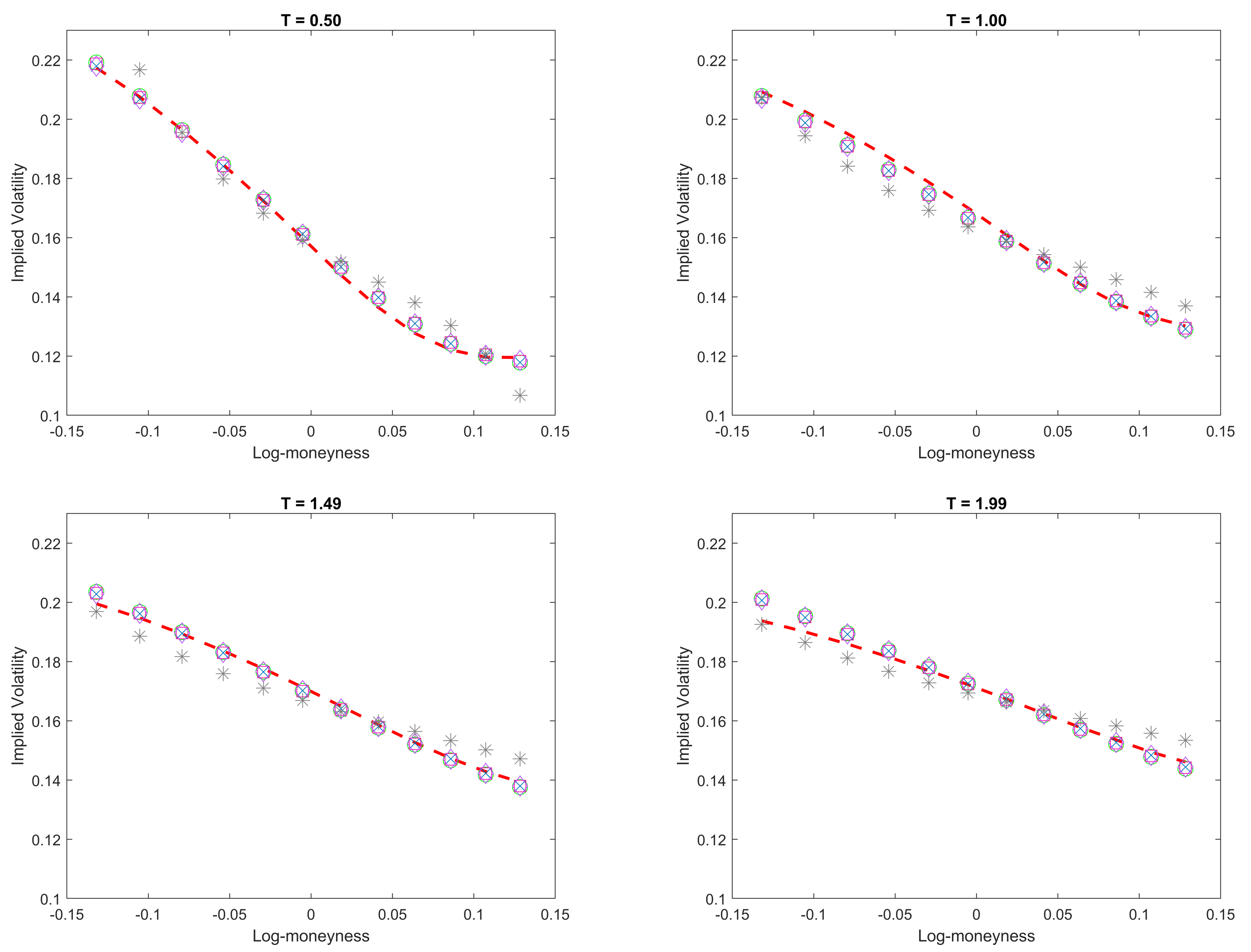
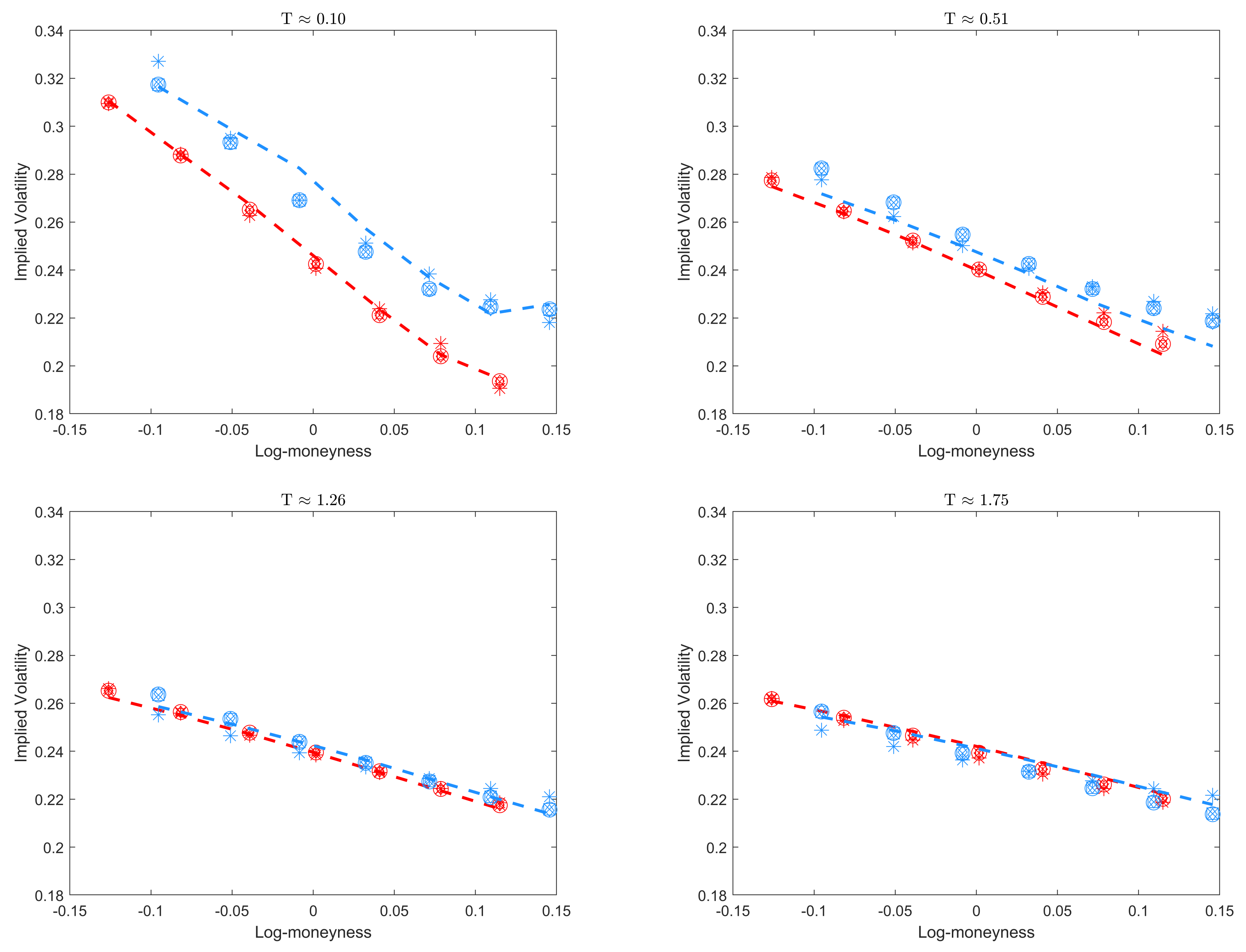
We perform numerical experiment in Section 4. The numerical experiment is tested on two different scenarios, a normal day and a major catastrophic event, the Lehman Brothers collapse. It is found that under non-extreme market condition, the OGPadé, OFPadé (5,4) (6,3), (7,2) performed similarly to one another and it has better performance than the approximation formula (19). In extreme market condition, the methods OGPadé, OFPadé, and approximation formula have reduced accuracy in matching the SPX implied volatility, but nevertheless, they are still capable of mimicking the SPX implied volatility surface.

References

1. Black, F.; Scholes, M. The pricing of options and corporate liabilities. World Scientific Reference on Contingent Claims Analysis in Corporate Finance: Volume 1: Foundations of CCA and Equity Valuation; World Scientific: Singapore, 2019; pp. 3–21. [Google Scholar]
2. Merton, R.C. Option pricing when underlying stock returns are discontinuous. J. Financ. Econ. 1976, 3, 125–144. [Google Scholar] [CrossRef] [Green Version]
3. Hull, J.; White, A. Pricing interest-rate-derivative securities. Rev. Financ. Stud. 1990, 3, 573–592. [Google Scholar] [CrossRef]
4. Heston, S.L. A closed-form solution for options with stochastic volatility with applications to bond and currency options. Rev. Financ. Stud. 1993, 6, 327–343. [Google Scholar] [CrossRef] [Green Version]
5. Fukasawa, M. Asymptotic analysis for stochastic volatility: Martingale expansion. Financ. Stoch. 2011, 15, 635–654. [Google Scholar] [CrossRef] [Green Version]
6. Gatheral, J. The Volatility Surface: A Practitioner’s Guide; John Wiley & Sons: Hoboken, NJ, USA, 2011; Volume 357. [Google Scholar]
7. Gatheral, J.; Jaisson, T.; Rosenbaum, M. Volatility is rough. Quant. Financ. 2018, 18, 933–949. [Google Scholar] [CrossRef]
8. Mandelbrot, B.B.; Van Ness, J.W. Fractional Brownian motions, fractional noises and applications. SIAM Rev. 1968, 10, 422–437. [Google Scholar] [CrossRef]
9. Bayer, C.; Friz, P.; Gatheral, J. Pricing under rough volatility. Quant. Financ. 2016, 16, 887–904. [Google Scholar] [CrossRef]
10. El Euch, O.; Fukasawa, M.; Rosenbaum, M. The microstructural foundations of leverage effect and rough volatility. Financ. Stoch. 2018, 22, 241–280. [Google Scholar] [CrossRef] [Green Version]
11. El Euch, O.; Rosenbaum, M. The characteristic function of rough Heston models. Math. Financ. 2019, 29, 3–38. [Google Scholar] [CrossRef] [Green Version]
12. Fukasawa, M.; Gatheral, J. A Rough SABR Formula. 2021. Available online: https://ssrn.com/abstract=3844278 (accessed on 2 August 2021).
13. Diethelm, K.; Ford, N.J.; Freed, A.D. Detailed error analysis for a fractional Adams method. Numer. Algorithms 2004, 1, 31–52. [Google Scholar] [CrossRef] [Green Version]
14. Carr, P.; Madan, D. Option valuation using the fast Fourier transform. Financ. J. Comput. Financ. 1999, 2, 61–73. [Google Scholar] [CrossRef] [Green Version]
15. Lewis, A.L. Option Valuation under Stochastic Volatility ii; Finance Press: Newport Beach, CA, USA, 2009. [Google Scholar]
16. Momani, S.; Shawagfeh, N. Decomposition method for solving fractional Riccati differential equations. Appl. Math. Comput. 2006, 182, 1083–1092. [Google Scholar] [CrossRef]
17. Momani, Z.M.; Shaher, M. Application of variational iteration method to nonlinear differential equations of fractional order. Int. J. Nonlinear Sci. Numer. Simul. 2006, 7, 27–34. [Google Scholar]
18. Odibat, Z.; Momani, S. Modified homotopy perturbation method: Application to quadratic Riccati differential equation of fractional order. Chaos Solitons Fractals 2008, 36, 167–174. [Google Scholar] [CrossRef]
19. Cang, J.; Tan, Y.; Xu, H.; Liao, S.J. Series solutions of non-linear Riccati differential equations with fractional order. Chaos Solitons Fractals 2008, 40, 1–9. [Google Scholar] [CrossRef]
20. Gatheral, J.; Radoicic, R. Rational approximation of the rough Heston solution. Int. J. Theor. Appl. Financ. 2019, 22, 1950010. [Google Scholar] [CrossRef]
21. Jeng, S.W.; Kilicman, A. Fractional Riccati Equation and Its Applications to Rough Heston Model Using Numerical Methods. Symmetry 2020, 12, 959. [Google Scholar] [CrossRef]
22. Jeng, S.W.; Kilicman, A. Series Expansion and Fourth-Order Global Padé Approximation for a Rough Heston Solution. Mathematics 2020, 8, 1968. [Google Scholar] [CrossRef]
23. Jeng, S.W.; Kilicman, A. Approximation formula for option prices under rough heston model and short-time implied volatility behaviour. Symmetry 2020, 12, 1878. [Google Scholar] [CrossRef]
24. El Euch, O.; Rosenbaum, M. Perfect hedging in rough Heston models. Ann. Appl. Probab. 2018, 28, 3813–3856. [Google Scholar] [CrossRef] [Green Version]
25. Jaisson, T.; Rosenbaum, M. Rough fractional diffusions as scaling limits of nearly unstable heavy tailed Hawkes processes. Ann. Appl. Probab. 2016, 26, 2860–2882. [Google Scholar] [CrossRef] [Green Version]
26. Gatheral, J.; Keller-Ressel, M. Affine forward variance models. Financ. Stoch. 2018, 23, 501–533. [Google Scholar] [CrossRef] [Green Version]
27. Alos, E.; Gatheral, J.; Radoičić, R. Exponentiation of conditional expectations under stochastic volatility. Quant. Financ. 2020, 20, 13–27. [Google Scholar] [CrossRef]
28. Baschetti, F.; Bormetti, G.; Romagnoli, S.; Rossi, P. Rough Heston: The SINC way. arXiv 2020, arXiv:2009.00557. [Google Scholar] [CrossRef]
29. Cherubini, U.; Della Lunga, G.; Mulinacci, S.; Rossi, P. Fourier Transform Methods in Finance; John Wiley & Sons: Hoboken, NJ, USA, 2010; Volume 524. [Google Scholar]
30. Alòs, E. A decomposition formula for option prices in the Heston model and applications to option pricing approximation. Financ. Stoch. 2012, 16, 403–422. [Google Scholar] [CrossRef] [Green Version]
31. Alòs, E.; De Santiago, R.; Vives, J. Calibration of stochastic volatility models via second-order approximation: The Heston case. Int. J. Theor. Appl. Financ. 2015, 18, 1550036. [Google Scholar] [CrossRef]
Figure 1. Implied volatility surface calibration on the SPX implied volatility (18 June 2021—dashed red line) for the OGPadé (diamond marker), OFPadé approximants ( 5 , 4 ) , ( 6 , 3 ) , ( 7 , 2 ) (square, cross, circle marker), and approximation formula (asterisk marker).
Mathematics 09 02675 g001
Figure 2. Implied volatility surface calibration on the SPX implied volatility (12 and 15 September 2008—dotted red and blue line) for the OGPadé (diamond marker), OFPadé approximants ( 5 , 4 ) , ( 6 , 3 ) , ( 7 , 2 ) (square, cross, circle marker), and approximation formula (asterisk marker).
Mathematics 09 02675 g002