On K-Means Clustering with IVIF Datasets for Post-COVID-19 Recovery Efforts

Abstract

The recovery efforts of the tourism and hospitality sector are compromised by the emergence of COVID-19 variants that can escape vaccines. Thus, maintaining non-pharmaceutical measures amidst massive vaccine rollouts is still relevant. The previous works which categorize tourist sites and restaurants according to the perceived degree of tourists’ and customers’ exposure to COVID-19 are deemed relevant for sectoral recovery. Due to the subjectivity of predetermining categories, along with the failure of capturing vagueness and uncertainty in the evaluation process, this work explores the use $k$-means clustering with dataset values expressed as interval-valued intuitionistic fuzzy sets. In addition, the proposed method allows for the incorporation of criteria (or attribute) weights into the dataset, often not considered in traditional $k$-means clustering but relevant in clustering problems with attributes having varying priorities. Two previously reported case studies were analyzed to demonstrate the proposed approach, and comparative and sensitivity analyses were performed. Results show that the priorities of the criteria in evaluating tourist sites remain the same. However, in evaluating restaurants, customers put emphasis on the physical characteristics of the restaurants. The proposed approach assigns 12, 15, and eight sites to the “low exposure”, “moderate exposure”, and “high exposure” cluster, respectively, each with distinct characteristics. On the other hand, 16 restaurants are assigned “low exposure”, 16 to “moderate exposure”, and eight to “high exposure” clusters, also with distinct characteristics. The characteristics described in the clusters offer meaningful insights for sectoral recovery efforts. Findings also show that the proposed approach is robust to small parameter changes. Although idiosyncrasies exist in the results of both case studies, considering the characteristics of the resulting clusters, tourists or customers could evaluate any tourist site or restaurant according to their perceived exposure to COVID-19.

1. Introduction

The current pandemic has adversely impacted the tourism and hospitality industry through travel restrictions and physical distancing measures. Following these prolonged measures, tourists’ behavior after reopening is linked to their perceived degree of exposure to COVID-19 [1,2]. The perceived degree of exposure may vary depending on the characteristics associated with the tourist sites and the hospitality establishments under consideration. For instance, the proximity of the destination, the duration of stay, and the volume of tourist arrivals may prompt the difference in the degree of exposure to COVID-19. Gaining insights on the degree of exposure is crucial for the decision-makers in implementing measures that would mitigate the fear of travel and reverberate the entire tourism value chain. This agenda has been explored in the recent work of Yamagishi and Ocampo [2], with subsequent and more comprehensive reports of Ocampo and Yamagishi [3] and Ocampo et al. [4]. They adopted an approach based on multi-attribute decision-making (MADM) methods in sorting tourist sites (restaurants) for perceived COVID-19 exposure of tourists (customers) under multiple relevant criteria. Their approaches involve the introduction of various attributes that would evaluate numerous alternatives (e.g., tourist sites, restaurants) under a computational platform that would capture the subjectivity and uncertainty of the evaluation environment. Their work allows the evaluation of the susceptibility of tourists to COVID-19 infection when visiting tourist sites, which is a relevant recovery effort of the industry.

While previous works [2,3,4] reported an interesting agenda for tourism and hospitality recovery, their approach may suffer certain drawbacks. First, the multiple criteria sorting methods employed in both studies in sorting tourist sites into classes are highly susceptible to subjective bias. In sorting methods, the characteristics of classes are predetermined by the analyst or by the decision-makers. The limited knowledge and inclinations of the analyst likely impose a bias on defining the classes and, in turn, on the overall sorting process. This drawback can be overcome by using clustering instead of sorting. In clustering, the characteristics of the clusters are determined by the shared characteristics of the alternatives that the clustering algorithm assigns to the cluster. With it, the need to predetermine the characteristics of clusters is eliminated along with the bias that it introduces. Secondly, their evaluation platform failed to account for a more encompassing agenda in addressing vagueness and uncertainty in the evaluation process. Such a limited approach in capturing judgment uncertainty brought about by factors such as the incomplete knowledge and experience of decision-makers with the problem domain may yield counterintuitive results. Reports in the literature suggest that capturing vagueness and uncertainty in decision-making represents a more robust and representative approach in addressing evaluation problems [4], particularly with those agendas having crucial impacts (e.g., public health). This work advances these gaps by offering a methodology in clustering a pre-determined number of alternatives or destinations (e.g., tourist sites, restaurants) based on the customers’ perception of their degree of exposure to COVID-19.

In this work, the same problem domain reported by our previous works [3,4] is addressed through clustering analysis, where homogeneous decision clusters are determined by the similarity of the alternatives (e.g., tourist sites, restaurants). Clustering describes a process of grouping a set of objects into classes of similar characteristics such that the objects within a given group should be similar to each other, whereas the objects within different groups should be dissimilar to each other. It has been extensively used in many areas such as image processing and segmentation [5], data mining [6], pattern recognition [7], among others. Clustering algorithms can be broadly divided into two groups: hierarchical and partitional. This work utilizes a partitioning clustering algorithm that simultaneously finds all the clusters as partitions of the data and does not impose a hierarchical structure. A partitional algorithm can use either an $n\times d$ pattern matrix, where $n$ objects are embedded in a $d$-dimensional feature space, or an $n\times n$ similarity matrix. The most popular partitional clustering algorithm in various domains is the $k$-means clustering, first introduced by Mac Queen in 1967. It has been widely used in several applications, such as environmental science [8], education [9], medicine [10], transportation [11], tourism [12,13], among others. In most applications in the literature, little regard is placed on the relative importance of the attributes of the observations that are being clustered. Only very few consider such an essential aspect of the clustering process [14,15]. In most applications, the assumption of equal attribute importance is implicitly invoked. However, this assumption might be unsuitable in some cases. For instance, each criterion may present a different priority to the decision-maker for clustering alternatives (i.e., considered as observations) based on multiple criteria [15]. This issue is addressed in this study by pre-processing data inputs for the $k$-means clustering to incorporate weights representing the importance of the attributes (i.e., criteria).

Moreover, when $k$-means clustering is associated with a dataset obtained from human judgments, evaluation scores expressed in crisp values would yield limited information on the uncertainty of the decision-making process. Thus, in this work, linguistic variables representative of those scores are introduced with corresponding interval-valued intuitionistic fuzzy (IVIF) sets. In many practical decision-making problems, the decision-makers often provide their preferences over a list of alternatives. This preference is usually imprecise or uncertain, along with the hesitation about the preference due to several factors such as lack of sufficient information or decision-makers having limited information processing capacities [16]. The rise of the use of fuzzy sets in data management has been popular in addressing this concern. Zadeh [17] first proposed the notion of a fuzzy set to model qualitative information with non-sharp boundaries, and Atanassov [18] generalized this idea to intuitionistic fuzzy set (IFS) by introducing both membership and non-membership degrees, extending the previous proposal of Zadeh [17] on membership functions to represent a fuzzy set. The use of IFS in modeling uncertainty has been widespread in the recent decade [19]. However, the membership and non-membership degrees in IFS are expressed as crisp values with limited capability in completely representing uncertainty and hesitation. Thus, Atanassov and Gargov [20] introduced interval membership and non-membership degrees, coining the term interval-valued intuitionistic fuzzy set (IVIFS). Recent works on the use of IVIFS values have been emerging in various applications, such as energy systems [21], medical diagnosis [22], image processing [23], transportation [24], tourism [25], hospitality [26], among others. Note that this list is not intended to be comprehensive. The integration of IVIFS in the datasets for $k$-means clustering augments the representation of judgment uncertainty involved in evaluation problems that attempt to identify resultant clusters of decision alternatives. In summary, this work contributes by (1) introducing a platform for $k$-means clustering based on datasets with IVIFS values, and (2) applying such a platform to advance our previous works [3,4] in tourism and hospitality recovery efforts.

This paper is outlined as follows: Section 2 provides a brief literature review of the recovery efforts of the tourism and hospitality sector. Section 3 illustrates the preliminaries of IVIFS and $k$-means clustering. Section 4 presents the application of the proposed $k$-means clustering with IVIFS datasets in two case studies in the Philippines. The sensitivity of the results, along with the comparative analysis on the performance of the proposed approach with the VIKORSORT and IF-TOPSIS-Sort, is presented in Section 5. It proceeds with a discussion of findings in Section 6. It ends with a conclusion and discussion of future works in Section 7.

2. Literature Review

A highly transmittable disease identified as coronavirus disease 2019 (COVID-19) with symptoms such as fever, dry cough, fatigue, shortness of breath, chills, muscles pain, headache, gastric discomforts, and weight loss was declared as a global pandemic on the 11 of March 2020 by the World Health Organization (WHO) [27,28]. Since its emergence in Wuhan, China, in November 2019, a total of 195 million confirmed cases of COVID-19, including 4 million deaths as of July 2021, has been recorded (WHO) [29]. To mitigate the spread of the virus and “flatten the curve”, non-pharmaceutical measures such as travel and mobility restrictions, social distancing protocols, and community lockdowns have been imposed globally [30]. The Organization for Economic Co-operation and Development (OCED) pointed out that the tourism sector was among the first industries highly affected by the coronavirus outbreak [31]. Before the pandemic, the collective direct, indirect, and induced contributions of the tourism industry accounted for 10.6% of all jobs and 10.4% of global GDP [32]. The tourism industry thrives through physical visits and face-to-face interactions, and its growth relies heavily on demand for its goods and services. Due to travel bans, event cancellations, quarantine requirements, and fear of spread, the industry faces commercial, operational, and financial crises [33]. Records in 2020 indicate that the unemployment rate has increased by approximately 18.5%, while the global GDP contribution of the industry decreased to 5.5% due to ongoing restrictions on mobility [32].

A case in point, the Philippine government recognizes the tourism sector as the most vulnerable amidst the COVID-19 pandemic. For the full-year report of 2020, the direct GDP contribution of the tourism industry is only Php 973.31 billion (19.53 billion USD), lower by 61.2% compared to Php 2.51 trillion (50.35 billion USD) of 2019 [34]. The decline of the GDP was caused by the restrictions imposed by the government to ensure the safety of the people, such as lowering the operational capacity of the establishment to enable social distancing measures. In fact, a survey conducted by the Asia Development Bank [35] for the Philippines reported that 89.9% of the businesses in the hospitality sector are not more than 50% operational, while 22.2% of them are now permanently closed. Consequently, the hospitality sector has a −42.7% GDP growth in 2020 and is among the main contributors to the decline of the country’s GDP [36]. Furthermore, restricted operations of the sector resulted in a 17.98% decrease in the labor force [37]. Thus, both tourism and labor and employment departments led the Financial Assistance and Cash-for-Work Program, providing financial support for displaced workers in the tourism industry, including the hospitality sector.

Amidst the enormous blow, industry decision-makers endeavor to promote initiatives that serve as coping mechanisms until some stability is obtained. These initiatives include robust negotiations with suppliers for sustenance, extensive cost reduction practices, or a minimum mandatory period for accommodation bookings when visiting tourist destinations and hospitality businesses [38]. For customer safety, restaurants and food establishments implement proactive measures, such as contactless menu boards, payment systems, changed sitting arrangements, health checks of diners, and regular sanitation of chairs and tables [39]. At record speed, the development and deployment of COVID-19 vaccines open a critical window to fight the COVID-19 pandemic and promote the safe resumption of international travel alongside other risk mitigation tools such as COVID-19 testing [40]. As of July 2021, approximately 4 billion doses of vaccines have been administered worldwide [41]. According to Gursoy et al. [42], COVID-19 vaccines have significantly raised the hopes for recovery as they can effectively mitigate the disease spread, which would lead to lifting global travel bans and improving the demand for tourism and hospitality products. Even though vaccination can speed up socio-economic recovery, several factors hinder countries from attaining herd immunity, including the willingness of the population to get vaccinated, lack of resources (e.g., budget), and improper allocation of doses [43,44].

However, alongside the introduction of vaccines and the consequent relaxation of preventive measures (e.g., restricted outings, avoidance of gatherings, self-isolation, and lockdowns), a quick escalation of COVID-19 cases across Europe arises. As a response, governments reimpose measures that would limit social activities to counter succeeding waves of COVID-19 [45]. The second wave of COVID-19 cases made way for the viral mutation and emergence of new variants (e.g., Alpha variant, Delta variant), more contagious and fatal than their parent virus [46]. The existence of new COVID-19 variants has been threatening countries in achieving herd immunity and inducing a reduced sense of safety for tourists to travel [45]. Thus, despite heightened vaccine rollouts, the tourism and hospitality sector needs a set of recovery efforts that would still maintain a certain degree of non-pharmaceutical measures. Our recently reported works [2,3,4] explored this agenda by evaluating the degree of exposure of tourists or customers in the facilities managed by the sector (i.e., tourist sites, restaurants. The computational platforms demonstrated in the previous works offer crucial insights to the sectoral recovery efforts in informing the design of measures of various stakeholders in managing the operations of the facilities. However, some methodological issues (e.g., the drawbacks of sorting items to pre-determined groups, the uncertainty of judgments) of these platforms are valid, which may require a different analytical perspective.

3. Preliminaries

3.1. Fuzzy Set Theory

Zadeh developed the fuzzy set theory in 1965, initially motivated by applying numerous valued logics as means of illustrating the behavior of complex electrical systems, which later turned into the idea of a fuzzy set [17]. In real-life scenarios, it is understood that conversations do not always lead to true or to false statements. Many statements exist between true and false, and these are called "statements of gradual truth" [47]. Fuzzy set theory is an established mathematical framework that measures uncertainties associated with vague and perception-based situations, opposing randomness [17]. It was derived from Boolean logic, where the absolute truth values 0 and 1 are described as being entirely false and entirely true, respectively. On the other hand, in the case of the fuzzy set theory, the degree of truth values assumes a closed interval $\left[0,1\right]$ defined by a membership function [17]. The notion of the framework of a fuzzy set provides a natural way of handling problems in which the lack of precisely defined criteria of class membership is the basis of indistinctness rather than the existence of random variables [17]. For an element that belongs to the fuzzy set $A$ in $X$, several possibilities such as "that element belongs to $A$", "partially belongs to $A$", and "does not belong to $A$" are applicable.

Definition 1:

Let$X$be the universe of discourse. The set of pairs$A=\left\{x,{\mu }_A\left(x\right)|x\in X\right\}$is called a fuzzy set, or standard fuzzy set, where${\mu }_A\left(x\right)$is the membership function of$x$in$A$. In a standard fuzzy set$A$, each element$x$is mapped to the closed interval$\left[0,1\right]$by${\mu }_A:X\to \left[0,1\right]$, which includes all real numbers between 0 and 1, including 0 and 1.

The membership function of $A$ can also be expressed as $A\left(x\right)\in \left[0,1\right]$. A fuzzy set can also be written as:

$$A=\left\{{\mu }_A\left(x\right)/x:x \in X\right\}$$

(1)

or:

$$A=\underset{x}{{\displaystyle \cup }}{\mu }_A\left(x\right)/x$$

(2)

Assuming that the elements are continuous, then the set can be expressed as:

$$A=\int {\mu }_A\left(x\right)/x$$

(3)

In the context of fuzzy set, the crisp set can be considered as a special case where the crisp interval $A=\left[a,b\right]\subseteq ℝ$, $a<b$, has a membership function ${\mu }_A\left(x\right)$ defined by:

$${\mu }_A\left(x\right)=\left\{\begin{array}{ll}0& \hspace{1em}x<a\\ 1& a\le x\le b\\ 0& \hspace{1em}x>b\end{array}\right.$$

(4)

3.2. Intuitionistic Fuzzy Set Theory

The intuitionistic fuzzy set theory, introduced by Atanassov [18], generalizes the fuzzy set theory of Zadeh [17] for computing information with vagueness and impression. It extends the fuzzy set theory by introducing a non-membership function in addition to the membership function and a resulting hesitancy function [18]. The non-membership function expresses opposition, while the hesitancy function represents neutrality in eliciting information. These additional components improve the efficacy of fuzzy computing, particularly in applications that require making decisions under uncertainty. The fundamentals of the IFS theory can be found in Atanassov [48] and several succeeding foundational works thereafter. For brevity, the following provides some useful and relevant concepts.

Definition 2 

([18]).Suppose$X$is a finite, non-empty set. Then an intuitionistic fuzzy set$A$in$X$is defined as:

$$A=\left\{x,{\mu }_A\left(x\right),{\nu }_A\left(x\right):x\in X\right\},$$

(5)

where${\mu }_A\left(x\right):X\to \left[0,1\right]$and${\nu }_A\left(x\right):X\to \left[0,1\right]$such that$0\le {\mu }_A\left(x\right)+{\nu }_A\left(x\right)\le 1,\forall x\in X$. Here, two mappings of$x\in X$to$A$are introduced: (1) the membership function${\mu }_A\left(x\right)$, and (2) the non-membership function${\nu }_A\left(x\right)$. From these functions, the hesitancy function${\pi }_A\left(x\right)$, i.e., the degree of the lack of knowledge on$x$in$A$, is generated and is defined as${\pi }_A\left(x\right)=1-{\mu }_A\left(x\right)-{\nu }_A\left(x\right)$.

Definition 3

([20]).Let$D\left[0,1\right]$be the set of all closed subintervals of$\left[0,1\right]$. Let$X\ne \varnothing$be a given set. An interval-valued intuitionistic fuzzy (IVIF) set$A$in$X$is given by$A=\left\{x,{\mu }_A^I\left(x\right),{\gamma }_A^I\left(x\right):x\in X\right\}$, where${\mu }_A^I\left(x\right):X⟶D\left[0,1\right]$,${\gamma }_A^I\left(x\right)⟶D\left[0,1\right]$, with the condition that

$$0<su{p}_x{\mu }_A^I\left(x\right)+su{p}_x{\gamma }_A^I\left(x\right)<1$$

(6)

The intervals${\mu }_A^I\left(x\right)$and${\gamma }_A^I\left(x\right)$, respectively, denote the degree of membership and non-membership of$x$to the set$A$.

For each $x\in X$, ${\mu }_A^I\left(x\right)$ and ${\gamma }_A^I\left(x\right)$ are closed intervals whose lower- and upper-end points are, respectively, denoted by ${\mu }_{AL}^I\left(x\right)$, ${\mu }_{AU}^I\left(x\right)$ and ${\gamma }_{AL}^I\left(x\right)$, ${\gamma }_{AU}^I\left(x\right)$. With these, $A$ can be written as $=\left\{x,\left[{\mu }_{AL}^I\left(x\right),{\mu }_{AU}^I\left(x\right)\right],\left[{\gamma }_{AL}^I\left(x\right), {\gamma }_{AU}^I\left(x\right)\right]:x\in X\right\}$, where $0\le {\mu }_{AL}^I\left(x\right)$, $0\le {\gamma }_{AL}^I\left(x\right)$, and $0<{\mu }_{AU}^I\left(x\right)+{\gamma }_{AU}^I\left(x\right)\le 1$.

For each $x\in X$, the hesitancy degree ${\pi }_A\left(x\right)$ of $x\in X$ in $A$ is defined as follows:

$${\pi }_A^I\left(x\right)=1-{\mu }_A^I\left(x\right)-{\gamma }_A^I\left(x\right)=\left[1-{\mu }_{AU}^I\left(x\right)-{\gamma }_{AU}^I\left(x\right),1-{\mu }_{AL}^I\left(x\right)-{\gamma }_{AL}^I\left(x\right)\right]$$

(7)

We will denote IVIFS $\left(X\right)$ as the set of all IVIF sets in $X$. For convenience, we will write the IVIFS value $A=\left(\left[a,b\right],\left[c,d\right]\right)$.

Definition 4 

([49,50]).Let$A=\left(\left[a,b\right],\left[c,d\right]\right)$,$A_1=\left(\left[a_1,b_1\right],\left[c_1,d_1\right]\right)$, and$A_2=\left(\left[a_2,b_2\right],\left[c_2,d_2\right]\right)$be IVIFS values, and$\lambda >0$. The following shows some of their basic operational laws:

$$1-A=A^c=\left(\left[c,d\right],\left[a,b\right]\right)$$

(8)

$$A_1\cup A_2=\left(\left[\max \left(a_1,a_2\right),\max \left(b_1,b_2\right)\right],\left[\min \left(c_1,c_2\right),\min \left(d_1,d_2\right)\right]\right)$$

(9)

$$A_1\cap A_2=\left(\left[\min \left(a_1,a_2\right),\min \left(b_1,b_2\right)\right],\left[\max \left(c_1,c_2\right),\max \left(d_1,d_2\right)\right]\right)$$

(10)

$$A_1+A_2=\left(\left[a_1+a_2-a_1{a}_2,b_1+b_2-b_1{b}_2\right],\left[c_1{c}_2,d_1{d}_2\right]\right)$$

(11)

$$A_1\cdot A_2=\left(\left[a_1{a}_2,b_1{b}_2\right],\left[c_1+c_2-c_1{c}_2,d_1+d_2-d_1{d}_2\right]\right)$$

(12)

$$\lambda A=\left(\left[1-{\left(1-a\right)}^{\lambda },1-{\left(1-b\right)}^{\lambda }\right],\left[c^{\lambda },d^{\lambda }\right]\right)$$

(13)

$$A^{\lambda }=\left(\left[a^{\lambda },b^{\lambda }\right],\left[1-{\left(1-c\right)}^{\lambda },1-{\left(1-d\right)}^{\lambda }\right]\right)$$

(14)

The following provides the two major approaches of aggregating IVIFS values: (1) the weighted arithmetic average operator and (2) the weighted geometric average operator.

Definition 5

([49]).Let$A_j\left(1,\dots ,n\right)\in IVIFS\left(X\right)$. The weighted arithmetic average operator ($F_w$) is defined by:

$$F_w=\left(A_1,\dots ,A_n\right)={{\displaystyle \sum }}_{j=1}^n{w}_j{A}_j=\left[1-{{\displaystyle \prod }}_{j\in \left\{1,...,n\right\}}{\left(1-{\mu }_{A_{j}L}^I\left(x\right)\right)}^{w_j},1-{{\displaystyle \prod }}_{j\in \left\{1,...,n\right\}}{\left(1-{\mu }_{A_{j}U}^I\left(x\right)\right)}^{w_j}\right],\left[\left({{\displaystyle \prod }}_{j\in \left\{1,...,n\right\}}{\left({\gamma }_{A_{j}L}^I\left(x\right)\right)}^{w_j}\right),\left({{\displaystyle \prod }}_{j\in \left\{1,...,n\right\}}{\left({\gamma }_{A_{j}U}^I\left(x\right)\right)}^{w_j}\right)\right]$$

(15)

where$w_j$is the weight of$A_j\left(1,\dots ,n\right)$,$w_j\in \left[0,1\right]$,${\displaystyle \sum }_{j=1}^n{w}_j=1$.

Definition 6 (

[49]). Let $A_j\left(1,\dots ,n\right)\in IVIFS\left(X\right)$. The weighted geometric average operator ($G_w$) is defined by

$$G_w=\left(A_1,\dots ,A_n\right)={{\displaystyle \sum }}_{j=1}^n{w}_j{A}_j=\left(\left[\left({{\displaystyle \prod }}_{j\in \left\{1,...,n\right\}}{\left({\mu }_{A_{j}L}^I\left(x\right)\right)}^{w_j}\right),\left({{\displaystyle \prod }}_{j\in \left\{1,...,n\right\}}{\left({\mu }_{A_{j}U}^I\left(x\right)\right)}^{w_j}\right)\right],,,\left[1-{{\displaystyle \prod }}_{j\in \left\{1,...,n\right\}}{\left(1-{\gamma }_{A_{j}L}^I\left(x\right)\right)}^{w_j},1-{{\displaystyle \prod }}_{j\in \left\{1,...,n\right\}}{\left(1-{\gamma }_{A_{j}U}^I\left(x\right)\right)}^{w_j}\right]\right)$$

(16)

where $w_j$ is the weight of$A_j\left(1,\dots ,n\right)$,$w_j\in \left[0,1\right]$,${\displaystyle \sum }_{j=1}^n{w}_j=1$

The following discusses various approaches in comparing IVIFS values.

Definition 7 (

[49]). Let $A=\left(\left[a,b\right],\left[c,d\right]\right)$ be an IVIFS value, where$0\le a\le b\le 1$,$0\le c\le d\le 1$, and$b+d\le 1$. A score function$S\left(A\right)$ is defined as:

$$S\left(A\right)=\frac{\left(a-b\right)+\left(c-d\right)}{2}$$

(17)

where$S\left(A\right)\in \left[0,1\right]$

Definition 8

([49]).[Let$A=\left(\left[a,b\right],\left[c,d\right]\right)$be an IVIFS value, where$0\le a\le b\le 1$,$0\le c\le d\le 1$, and$b+d\le 1$. An accuracy function$H\left(A\right)$based on an unknown degree is defined as:

$$H\left(A\right)=\frac{\left(a+b\right)+\left(c+d\right)}{2}$$

(18)

where$H\left(A\right)\in \left[0,1\right]$.

Based on Definitions 7 and 8, Xu and Jian [39] proposed an approach to compare two IVIFS values. Theorem 1 offers such an approach.

Theorem 1 (

[51]). Let $A_1=\left(\left[a_1,b_1\right],\left[c_1,d_1\right]\right)$ and$A_2=\left(\left[a_2,b_2\right],\left[c_2,d_2\right]\right)$ be two IVIFS values. Then:

(i)

If$S\left(A_1\right)<S\left(A_2\right)$, then$A_1<A_2$

(ii)

If$S\left(A_1\right)=S\left(A_2\right)$, then:

• If$H\left(A_1\right)=H\left(A_2\right)$, then$A_1=A_2$
• If$H\left(A_1\right)<H\left(A_2\right)$, then$A_1<A_2$

Ye [52] offered a new formulation of the accuracy function (i.e., the novel accuracy function) that allows comparison among IVIFS values.

Definition 9 (

[52]). Let $A=\left(\left[a,b\right],\left[c,d\right]\right)$ be an IVIFS value, where$0\le a\le b\le 1$,$0\le c\le d\le 1$, and$b+d\le 1$. A novel accuracy function of in IVIFS values, based on an unknown degree, is proposed as:

$$M\left(A\right)=\frac{a-\left(1-a-c\right)+b-\left(1-b-d\right)}{2}=a+b-1+\frac{c+d}{2}$$

(19)

where $M\left(A\right)\in \left[-1,+1\right]$.

Shown in various examples, the novel accuracy function demonstrates a promising approach that improves the efficacy of the formulation proposed by Xu and Jian [51]. However, Nayagam et al. [53] argued that the previous two formulations might fail to compare IVIFS values in some instances. Thus, they devised an alternative formulation of an accuracy function.

Definition 10 (

[53]). Let $A=\left(\left[a,b\right],\left[c,d\right]\right)$ be an IVIFS value, where$0\le a\le b\le 1$,$0\le c\le d\le 1$, and$b+d\le 1$. A novel accuracy function$L\left(A\right)$ of in IVIFS values, based on an unknown degree, can be formulated as:

$$L\left(A\right)=\frac{a+b-d\left(1-b\right)-c\left(1-a\right)}{2}$$

(20)

where $L\left(A\right)\in \left[-1,+1\right]$.

Given Definition 10, the following result provides a basis for comparing two IVIFS values.

Theorem 2 (

[53]). For any two comparable IVIFS values $A$ and$B$ , if$A\le B$ , then$L\left(A\right)\le L\left(B\right)$.

3.3. K-Means Clustering

Clustering divides a set of data into clusters. Several clustering methods were employed for a variety of applications in the literature. Abualigah et al. [54] proposed an improved krill herd algorithm for text clustering. Janani and Vijayarani [55] employed the spectral clustering algorithm with particle swarm optimization for text document clustering. Ramirez et al. [56] employed the $k$-means clustering algorithm to determine clusters of education graduate students based on motivation. Selerio et al. [57] employed the fuzzy C-means clustering to improve sustainable urban water management. Although clustering algorithms are found to be useful in various domains, their application in tourism and hospitality recovery is not well explored. Among multiple algorithms, the $k$-means clustering algorithm is arguably the most popular due to its simplicity and strong theoretical foundations. It has been used in various applications, such as analyzing customer behavior [58], in situ additive manufacturing process monitoring [59], seismic attribute selection [60], and intelligent broadcasting [61], to name a few. Here, a novel application of $k$-means clustering is demonstrated for tourism and hospitality recovery amidst the COVID-19 pandemic.

The $k$-means clustering divides a set of data into $k$ number of distinct clusters. The process is partitioned into phases. It determines the $k$ centroid in the first phase and then moves each point to the cluster with the closest centroid to the data point in the second phase. The Euclidean distance is widely used for determining the distance to the nearest centroid. It recalculates the new centroid of each cluster once the grouping is complete. Based on that centroid, a new Euclidean distance between each center and each data point is calculated, and the cluster’s points with the shortest Euclidean distance are assigned. The member objects and centroid of each cluster in the partition define it. The centroid of each cluster is where the sum of the distances between all the items in the cluster is the smallest. The $k$-means algorithm is an iterative technique that minimizes the sum of distances between each item and its cluster centroid over all clusters. The Lloyd-Forgy algorithm [62,63] is used in this work.

The general formulation of the algorithm is as follows: Given a set of observations $\left(x_1,x_2,\dots ,x_n\right)$ where each observation is a $d$-dimensional real vector, $k$-means clustering aims to partition the $n$ observations into $k\le n$ sets $S=\left\{S_1,S_2,\dots , S_k\right\}$ to minimize the within-cluster sum of squares (i.e., variance). The objective function is defined as follows:

$${\arg \min }_S{{\displaystyle \sum }}_{i=1}^k{{\displaystyle \sum }}_{x\in S_i}x-{\mu }_i{}^2={\arg \min }_S{{\displaystyle \sum }}_{i=1}^k\left|S_i\right| \mathrm{Var} S_i$$

(21)

where ${\mu }_i$ is the mean of the points in $S$. This is equivalent to minimizing the pairwise squared deviations of points in the same cluster, as illustrated:

$${\arg \min }_S{{\displaystyle \sum }}_{i=1}^k\frac{1}{2\left|S_i\right|} {{\displaystyle \sum }}_{x,y\in S_i}{||x-y||}^2$$

(22)

and the equivalence can be deducted from the identity presented as follows:

$${{\displaystyle \sum }}_{xϵ S_i}x-{\mu }_i{}^2={{\displaystyle \sum }}_{x\ne y\in S_i}{\left(x-{\mu }_i\right)}^T\left({\mu }_i-y\right)$$

(23)

4. Proposed Procedure: The Application of K-Means Clustering Based on IVIF Datasets

4.1. Case Study 1: Clustering Tourist Sites for Perceived COVID-19 Exposure

The Philippine government recognizes the tourism sector as the most vulnerable amidst the COVID-19 pandemic. Hundreds of thousands of people have been unemployed due to the Philippines’ extended and widespread lockdown. With careful relaxation of containment measures [64], the government pushes for economic recovery while keeping public health a priority. The Department of Tourism (DOT), the government’s tourism arm, has been emphasizing the need for tourist trust and confidence for a healthy recovery, highlighting the necessity of safety measures and stakeholder participation in ensuring that public health standards are met [65]. In this regard, some standard protocols across tourist destinations were released [66]. Furthermore, the DOT introduced a personalized package trip as a key to encouraging more Filipinos for domestic travel and a way of faster tourism recovery. They also welcome the approval of uniform travel protocols for all local government units (LGUs), although some require a COVID-19 test before travel [66].

As tourism activities slowly resume, health and safety are deemed primary among travelers, and vaccination is considered essential to the industry’s full recovery [67]. Vaccination is deemed a cost-effective measure to control the spread of pandemics and minimize economic losses [68]. Progress on the vaccination rollout in the country is forecasted to contribute a 4.5% economic growth in 2021, according to the Asian Development Bank [69]. Mass vaccination in the Philippines began in March 2021, and in July 2021, the Philippines already can administer 500,000 daily vaccine doses. With the continuing effort of the government to implement the inoculation of vaccines to the population, the economy is expected to reopen with more relaxed movement restrictions. However, authorities are almost in consensus about some required forms of social distancing and other non-pharmaceutical measures, despite the presence of vaccines. For instance, several states in the U.S. mandate an indoor mask. On the other hand, some states, such as Hawaii, Nevada, and Washington D.C., allow the exemption to fully vaccinated individuals only after at least two weeks of their last shot. Nevertheless, with the current threat brought about by the Delta variant and other emerging variants, the U.S. Centers for Disease Control and Prevention recommends that vaccinated people wear masks in indoor areas with high rates of COVID-19 transmission [70]. Thus, while implementing recovery efforts in the tourism sector, putting up measures and safeguards for the tourists and enterprises remains crucial amidst the emergence of COVID-19 variants that can escape vaccines.

With this, the agenda of evaluating tourists’ perceived degree of exposure to COVID-19 in tourist sites is deemed relevant for tourism recovery. To address the limitations of multiple criteria sorting methods adopted in previous works, the proposed $k$-means clustering based on datasets with IVIFS values is adopted. Following the previous problem of sorting 35 tourist sites under six evaluation criteria, the required computational steps are as follows:

Step 1: Identify the necessary criteria.

Yamagishi and Ocampo [2] identified six criteria representing the degree of exposure of tourists to COVID-19 in various tourist sites. These include proximity (C1), available modes of transportation (C2), duration of stay (C3), tourist activities (C4), area of the site’s premises (C5), and volume of tourist arrivals (C6). The process of identifying these criteria was discussed thoroughly [3] and is not repeated here for brevity. However, activities such as literature review, focus group discussions, expert interviews, and other group consensus-generating techniques may be necessary to identify these criteria.

Step 2: Determine the list of evaluation alternatives.

The alternatives are represented by 35 tourist sites under a local geographical region [3]. These tourist sites are participating in tourism recovery efforts via domestic tourism and were pre-selected for the study. In general, the selection of tourist sites is problem-specific and is within the scope of the interests of decision-makers.

Table 1. List of tourist sites [3].

Type	Code	Tourist Site	Type	Code	Tourist Site
Sun, sea, sand	S1	Sumilon island	Ecotourism	S18	Bojo river
	S2	Panagsama beach		S19	Sanctuaries in Olango
	S3	Sardine run		S20	Omagieca mangrove garden
	S4	Basdaku	Farm tourism	S21	AO farm gardens
	S5	Virgin island		S22	Eskapo Verde ecotourism
	S6	Malapascua island	Water-based tourism	S23	Oslob whale watching
	S7	Orongan beach resort		S24	Kawasan falls
	S8	Lambug beach		S25	Pescador island
	S9	Tingko beach		S26	Canyoneering
	S10	Camotes beach		S27	Cebu Ocean Park
Heritage and culture	S11	Fort San Pedro	Adventure tourism	S28	Danasan eco adventure park
	S12	Casa Gorordo		S29	Cebu safari
	S13	Yap-Sandiego museum		S30	Anjo World
	S14	Museo sa Sugbo	Park tourism	S31	Sirao flower garden
	S15	Parian museum		S32	Tops lookout
	S16	Sugbo Chinese heritage museum		S33	D’Family park
	S17	Mactan shrine		S34	Baluarte park
				S35	Lake Danao

shows the list of 35 tourist sites with their corresponding codes for easier recall. The comprehensive characteristics of these sites are previously illustrated [3].

Step 3: Determine the priority weights of the criteria.

The dataset reported in our previous work [3] involves respondents evaluating the importance of the six criteria within the context of COVID-19 exposure using a 9-point scale. Two hundred twenty-one (221) respondents participated in an online survey. To capture the vagueness and uncertainty within the dataset, the 9-point scale is provided with an equivalent linguistic evaluation scale with corresponding IVIFS values, as shown in

Table 2. Linguistic evaluation scale for the priority weights of the criteria.

Rating	Linguistic Variable	Equivalent IVIFS Value
1	Extremely irrelevant	([0,0.1],[0.8,0.9])
2	Very irrelevant	([0.2,0.2],[0.7,0.7])
3	Irrelevant	([0.3,0.4],[0.5,0.6])
4	Slightly irrelevant	([0.4,0.5],[0.5,0.5])
5	Fairly relevant	([0.5,0.5],[0.4,0.5])
6	Slightly relevant	([0.6,0.7],[0.2,0.3])
7	Relevant	([0.7,0.8],[0.2,0.2])
8	Very relevant	([0.8,0.8],[0.1,0.1])
9	Extremely relevant	([0.9,1],[0,0])

. The presence of IVIFS values allows the integration of two aspects of uncertainty prevalent in judgment mapping, i.e., the membership and non-membership degrees of the evaluation ratings.

Let $A_j^k=\left(\left[{\mu }_{A_j^{k}L}^I,{\mu }_{A_j^{k}U}^I\right],\left[{\gamma }_{A_j^{k}L}^I,{\gamma }_{A_j^{k}U}^I\right]\right)$ be the IVIFS value representing the perception of the $k$th decision-maker on the importance of the $j$th criterion. Using the weighted arithmetic average operator found in Definition 5, the IVIF weight $F_{A_j}$ of the criterion $j$ is computed as:

$$F_{A_j}=\left(\left[{\mu }_{A_{j}L}^I,{\mu }_{A_{j}U}^I\right],\left[{\gamma }_{A_{j}L}^I,{\gamma }_{A_{j}U}^I\right]\right)={{\displaystyle \sum }}_{k=1}^K{w}_k{A}_j^k=\left(\left[1-{{\displaystyle \prod }}_{k\in \left\{1,...,K\right\}}{\left(1-{\mu }_{A_j^{k}L}^I\right)}^{w_k},1-{{\displaystyle \prod }}_{k\in \left\{1,...,K\right\}}{\left(1-{\mu }_{A_j^{k}U}^I\right)}^{w_k}\right],\left[\left({{\displaystyle \prod }}_{k\in \left\{1,...,K\right\}}{\left({\gamma }_{A_j^{k}L}^I\right)}^{w_k}\right),\left({{\displaystyle \prod }}_{k\in \left\{1,...,K\right\}}{\left({\gamma }_{A_j^{k}U}^I\right)}^{w_k}\right)\right]\right)$$

(24)

where $K$ is the total number of decision-makers, and $w_k=\frac{1}{K}$ with the assumption that all $K$ decision-makers have equal significance to the problem domain. Note that the required operations in Equation (24) are described in Definition 4. Following the required computations, the IVIF weights are shown in

Table 3. The IVIF weights of the evaluation criteria of tourist sites.

Codes	Criteria	IVIF Weights	$\mathbf{Novel} \mathbf{Accuracy} \mathbf{Function} \mathit{L}\left(\mathit{A}\right)$	Rank
C1	Proximity	([0.9,1],[0,0])	0.950	1
C2	Available modes of transportation	([0.78,1],[0,0])	0.891	3
C3	Duration of stay	([0.75,1],[0,0])	0.875	6
C4	Tourist activities	([0.76,1],[0,0])	0.879	5
C5	Area of site premises	([0.76,1],[0,0])	0.880	4
C6	Volume of tourist arrivals	([0.82,1],[0,0])	0.912	2

. By way of the novel accuracy function $L\left(A\right)$ of Definition 10, Theorem 2 provides a way of ranking these criteria. Results show that proximity is on top of the list, followed by the volume of tourist arrivals, available modes of transportation, area of site premises, tourist activities, and duration of stay.

Step 4: Evaluate the relevance of the alternatives for all criteria.

The same set of respondents evaluated the relevance of the 35 tourist sites under the six criteria using the same 9-point scale. With the equivalent linguistic variables presented in Table 2, the resulting datasets contain IVIFS data, where each entry $f_{ij}^k=\left(\left[{\mu }_{f_{ij}^{k}L}^I,{\mu }_{f_{ij}^{k}U}^I\right],\left[{\gamma }_{f_{ij}^{k}L}^I,{\gamma }_{f_{ij}^{k}U}^I\right]\right)$ represents the IVIFS score of each tourist site $i\left(1,...,m\right)$ with respect to a criterion $j\left(1,\dots ,n\right)$ as perceived by the decision-maker $k\left(1,\dots ,K\right)$.

Table 4. Sample IVIF dataset representing a respondent evaluating the tourist sites.

Tourist Sites	C1	C2	C3	C4	C5	C6
S1	([0.4,0.5],[0.5,0.5])	([0.5,0.5],[0.4,0.5])	([0.5,0.5],[0.4,0.5])	([0.5,0.5],[0.4,0.5])	([0.4,0.5],[0.5,0.5])	([0.5,0.5],[0.4,0.5])
S2	([0.4,0.5],[0.5,0.5])	([0.5,0.5],[0.4,0.5])	([0.5,0.5],[0.4,0.5])	([0.5,0.5],[0.4,0.5])	([0.5,0.5],[0.4,0.5])	([0.5,0.5],[0.4,0.5])
S3	([0.7,0.8],[0.2,0.2])	([0.8,0.8],[0.1,0.1])	([0.9,1],[0,0])	([0.9,1],[0,0])	([0.8,0.8],[0.1,0.1])	([0.9,1],[0,0])
S4	([0.5,0.5],[0.5,0.5])	([0.5,0.5],[0.4,0.5])	([0.5,0.5],[0.4,0.5])	([0.5,0.5],[0.4,0.5])	([0.5,0.5],[0.5,0.5])	([0.5,0.5],[0.4,0.5])
S5	([0.5,0.5],[0.4,0.5])	([0.5,0.5],[0.4,0.5])	([0.5,0.5],[0.4,0.5])	([0.5,0.5],[0.4,0.5])	([0.5,0.5],[0.4,0.5])	([0.5,0.5],[0.4,0.5])
S6	([0.5,0.5],[0.4,0.5])	([0.5,0.5],[0.4,0.5])	([0.5,0.5],[0.4,0.5])	([0.5,0.5],[0.4,0.5])	([0.5,0.5],[0.4,0.5])	([0.5,0.5],[0.4,0.5])
S7	([0.6,0.7],[0.2,0.3])	([0.6,0.7],[0.2,0.3])	([0.6,0.7],[0.2,0.3])	([0.6,0.7],[0.2,0.3])	([0.6,0.7],[0.2,0.3])	([0.6,0.7],[0.2,0.3])
S8	([0.6,0.7],[0.2,0.3])	([0.6,0.7],[0.2,0.3])	([0.6,0.7],[0.2,0.3])	([0.6,0.7],[0.2,0.3])	([0.6,0.7],[0.2,0.3])	([0.6,0.7],[0.2,0.3])
S9	([0.7,0.8],[0.2,0.2])	([0.7,0.8],[0.2,0.2])	([0.7,0.8],[0.2,0.2])	([0.7,0.8],[0.2,0.2])	([0.7,0.8],[0.2,0.2])	([0.7,0.8],[0.2,0.2])
S10	([0.6,0.7],[0.2,0.3])	([0.6,0.7],[0.2,0.3])	([0.6,0.7],[0.2,0.3])	([0.6,0.7],[0.2,0.3])	([0.6,0.7],[0.2,0.3])	([0.6,0.7],[0.2,0.3])
S11	([0.7,0.8],[0.2,0.2])	([0.7,0.8],[0.2,0.2])	([0.7,0.8],[0.2,0.2])	([0.7,0.8],[0.2,0.2])	([0.7,0.8],[0.2,0.2])	([0.7,0.8],[0.2,0.2])
S12	([0.7,0.8],[0.2,0.2])	([0.7,0.8],[0.2,0.2])	([0.7,0.8],[0.2,0.2])	([0.7,0.8],[0.2,0.2])	([0.7,0.8],[0.2,0.2])	([0.7,0.8],[0.2,0.2])
S13	([0.7,0.8],[0.2,0.2])	([0.7,0.8],[0.2,0.2])	([0.7,0.8],[0.2,0.2])	([0.7,0.8],[0.2,0.2])	([0.7,0.8],[0.2,0.2])	([0.7,0.8],[0.2,0.2])
S14	([0.7,0.8],[0.2,0.2])	([0.7,0.8],[0.2,0.2])	([0.7,0.8],[0.2,0.2])	([0.7,0.8],[0.2,0.2])	([0.7,0.8],[0.2,0.2])	([0.7,0.8],[0.2,0.2])
S15	([0.7,0.8],[0.2,0.2])	([0.7,0.8],[0.2,0.2])	([0.7,0.8],[0.2,0.2])	([0.7,0.8],[0.2,0.2])	([0.7,0.8],[0.2,0.2])	([0.7,0.8],[0.2,0.2])
S16	([0.7,0.8],[0.2,0.2])	([0.7,0.8],[0.2,0.2])	([0.7,0.8],[0.2,0.2])	([0.7,0.8],[0.2,0.2])	([0.7,0.8],[0.2,0.2])	([0.7,0.8],[0.2,0.2])
S17	([0.7,0.8],[0.2,0.2])	([0.7,0.8],[0.2,0.2])	([0.7,0.8],[0.2,0.2])	([0.7,0.8],[0.2,0.2])	([0.7,0.8],[0.2,0.2])	([0.7,0.8],[0.2,0.2])
S18	([0.5,0.5],[0.4,0.5])	([0.5,0.5],[0.4,0.5])	([0.5,0.5],[0.4,0.5])	([0.5,0.5],[0.4,0.5])	([0.5,0.5],[0.4,0.5])	([0.5,0.5],[0.4,0.5])
S19	([0.5,0.5],[0.4,0.5])	([0.5,0.5],[0.4,0.5])	([0.5,0.5],[0.4,0.5])	([0.5,0.5],[0.4,0.5])	([0.5,0.5],[0.4,0.5])	([0.5,0.5],[0.4,0.5])
S20	([0.5,0.5],[0.4,0.5])	([0.5,0.5],[0.4,0.5])	([0.5,0.5],[0.4,0.5])	([0.5,0.5],[0.4,0.5])	([0.5,0.5],[0.4,0.5])	([0.5,0.5],[0.4,0.5])
S21	([0.7,0.8],[0.2,0.2])	([0.7,0.8],[0.2,0.2])	([0.7,0.8],[0.2,0.2])	([0.7,0.8],[0.2,0.2])	([0.7,0.8],[0.2,0.2])	([0.6,0.7],[0.2,0.3])
S22	([0.6,0.7],[0.2,0.3])	([0.6,0.7],[0.2,0.3])	([0.6,0.7],[0.2,0.3])	([0.6,0.7],[0.2,0.3])	([0.6,0.7],[0.2,0.3])	([0.7,0.8],[0.2,0.2])
S23	([0.7,0.8],[0.2,0.2])	([0.7,0.8],[0.2,0.2])	([0.7,0.8],[0.2,0.2])	([0.7,0.8],[0.2,0.2])	([0.7,0.8],[0.2,0.2])	([0.6,0.7],[0.2,0.3])
S24	([0.6,0.7],[0.2,0.3])	([0.6,0.7],[0.2,0.3])	([0.6,0.7],[0.2,0.3])	([0.6,0.7],[0.2,0.3])	([0.6,0.7],[0.2,0.3])	([0.5,0.5],[0.4,0.5])
S25	([0.5,0.5],[0.4,0.5])	([0.5,0.5],[0.4,0.5])	([0.5,0.5],[0.4,0.5])	([0.5,0.5],[0.4,0.5])	([0.5,0.5],[0.4,0.5])	([0.6,0.7],[0.2,0.3])
S26	([0.6,0.7],[0.2,0.3])	([0.6,0.7],[0.2,0.3])	([0.6,0.7],[0.2,0.3])	([0.6,0.7],[0.2,0.3])	([0.6,0.7],[0.2,0.3])	([0.7,0.8],[0.2,0.2])
S27	([0.7,0.8],[0.2,0.2])	([0.7,0.8],[0.2,0.2])	([0.7,0.8],[0.2,0.2])	([0.7,0.8],[0.2,0.2])	([0.7,0.8],[0.2,0.2])	([0.6,0.7],[0.2,0.3])
S28	([0.6,0.7],[0.2,0.3])	([0.6,0.7],[0.2,0.3])	([0.6,0.7],[0.2,0.3])	([0.6,0.7],[0.2,0.3])	([0.6,0.7],[0.2,0.3])	([0.5,0.5],[0.4,0.5])
S29	([0.5,0.5],[0.4,0.5])	([0.5,0.5],[0.4,0.5])	([0.5,0.5],[0.4,0.5])	([0.5,0.5],[0.4,0.5])	([0.5,0.5],[0.4,0.5])	([0.7,0.8],[0.2,0.2])
S30	([0.7,0.8],[0.2,0.2])	([0.7,0.8],[0.2,0.2])	([0.7,0.8],[0.2,0.2])	([0.7,0.8],[0.2,0.2])	([0.7,0.8],[0.2,0.2])	([0.6,0.7],[0.2,0.3])
S31	([0.6,0.7],[0.2,0.3])	([0.6,0.7],[0.2,0.3])	([0.6,0.7],[0.2,0.3])	([0.6,0.7],[0.2,0.3])	([0.6,0.7],[0.2,0.3])	([0.6,0.7],[0.2,0.3])
S32	([0.6,0.7],[0.2,0.3])	([0.6,0.7],[0.2,0.3])	([0.6,0.7],[0.2,0.3])	([0.6,0.7],[0.2,0.3])	([0.6,0.7],[0.2,0.3])	([0.7,0.8],[0.2,0.2])
S33	([0.7,0.8],[0.2,0.2])	([0.7,0.8],[0.2,0.2])	([0.7,0.8],[0.2,0.2])	([0.6,0.7],[0.2,0.3])	([0.7,0.8],[0.2,0.2])	([0.5,0.5],[0.4,0.5])
S34	([0.5,0.5],[0.4,0.5])	([0.5,0.5],[0.4,0.5])	([0.5,0.5],[0.4,0.5])	([0.5,0.5],[0.4,0.5])	([0.5,0.5],[0.4,0.5])	([0.5,0.5],[0.4,0.5])
S35	([0.5,0.5],[0.4,0.5])	([0.5,0.5],[0.4,0.5])	([0.5,0.5],[0.4,0.5])	([0.5,0.5],[0.4,0.5])	([0.5,0.5],[0.4,0.5])	([0.5,0.5],[0.4,0.5])

presents a sample dataset of a respondent in IVIFS values. The aggregate IVIFS score denoted by $f_{ij}$ is obtained as follows:

$$f_{ij}=\left(\left[{\mu }_{f_{ij}L}^I,{\mu }_{f_{ij}U}^I\right],\left[{\gamma }_{f_{ij}L}^I,{\gamma }_{f_{ij}U}^I\right]\right)=\left(\left[1-{{\displaystyle \prod }}_{k\in \left\{1,...,K\right\}}{\left(1-{\mu }_{f_{ij}^{k}L}^I\right)}^{w_k},1-{{\displaystyle \prod }}_{k\in \left\{1,...,K\right\}}{\left(1-{\mu }_{f_{ij}^{k}U}^I\right)}^{w_k}\right],\left[\left({{\displaystyle \prod }}_{k\in \left\{1,...,K\right\}}{\left({\gamma }_{f_{ij}^{k}L}^I\right)}^{w_k}\right),\left({{\displaystyle \prod }}_{k\in \left\{1,...,K\right\}}{\left({\gamma }_{f_{ij}^{k}U}^I\right)}^{w_k}\right)\right]\right)$$

(25)

where $w_k=\frac{1}{K}$. The aggregate dataset with IVIFS values is shown in

Table 5. Aggregate IVIF dataset for the evaluation of tourist sites.

Tourist Sites	C1	C2	C3	C4	C5	C6
S1	([0.63,1],[0,0])	([0.73,1],[0,0])	([0.66,1],[0,0])	([0.69,1],[0,0])	([0.67,1],[0,0])	([0.77,1],[0,0])
S2	([0.68,1],[0,0])	([0.73,1],[0,0])	([0.7,1],[0,0])	([0.72,1],[0,0])	([0.71,1],[0,0])	([0.78,1],[0,0])
S3	([0.65,1],[0,0])	([0.71,1],[0,0])	([0.67,1],[0,0])	([0.68,1],[0,0])	([0.68,1],[0,0])	([0.75,1],[0,0])
S4	([0.68,1],[0,0])	([0.74,1],[0,0])	([0.7,1],[0,0])	([0.72,1],[0,0])	([0.71,1],[0,0])	([0.78,1],[0,0])
S5	([0.64,1],[0,0])	([0.71,1],[0,0])	([0.66,1],[0,0])	([0.69,1],[0,0])	([0.69,1],[0,0])	([0.75,1],[0,0])
S6	([0.67,1],[0,0])	([0.72,1],[0,0])	([0.68,1],[0,0])	([0.7,1],[0,0])	([0.7,1],[0,0])	([0.76,1],[0,0])
S7	([0.63,1],[0,0])	([0.69,1],[0,0])	([0.66,1],[0,0])	([0.67,1],[0,0])	([0.67,1],[0,0])	([0.74,1],[0,0])
S8	([0.68,1],[0,0])	([0.72,1],[0,0])	([0.68,1],[0,0])	([0.7,1],[0,0])	([0.7,1],[0,0])	([0.77,1],[0,0])
S9	([0.66,1],[0,0])	([0.72,1],[0,0])	([0.67,1],[0,0])	([0.7,1],[0,0])	([0.71,1],[0,0])	([0.77,1],[0,0])
S10	([0.67,1],[0,0])	([0.72,1],[0,0])	([0.67,1],[0,0])	([0.7,1],[0,0])	([0.69,1],[0,0])	([0.77,1],[0,0])
S11	([0.74,1],[0,0])	([0.74,1],[0,0])	([0.71,1],[0,0])	([0.72,1],[0,0])	([0.76,1],[0,0])	([0.8,1],[0,0])
S12	([0.72,1],[0,0])	([0.74,1],[0,0])	([0.7,1],[0,0])	([0.72,1],[0,0])	([0.75,1],[0,0])	([0.79,1],[0,0])
S13	([0.7,1],[0,0])	([0.72,1],[0,0])	([0.69,1],[0,0])	([0.71,1],[0,0])	([0.74,1],[0,0])	([0.78,1],[0,0])
S14	([0.71,1],[0,0])	([0.73,1],[0,0])	([0.7,1],[0,0])	([0.72,1],[0,0])	([0.75,1],[0,0])	([0.78,1],[0,0])
S15	([0.73,1],[0,0])	([0.73,1],[0,0])	([0.7,1],[0,0])	([0.73,1],[0,0])	([0.75,1],[0,0])	([0.78,1],[0,0])
S16	([0.71,1],[0,0])	([0.72,1],[0,0])	([0.69,1],[0,0])	([0.71,1],[0,0])	([0.73,1],[0,0])	([0.77,1],[0,0])
S17	([0.71,1],[0,0])	([0.73,1],[0,0])	([0.68,1],[0,0])	([0.7,1],[0,0])	([0.72,1],[0,0])	([0.77,1],[0,0])
S18	([0.66,1],[0,0])	([0.7,1],[0,0])	([0.65,1],[0,0])	([0.69,1],[0,0])	([0.67,1],[0,0])	([0.74,1],[0,0])
S19	([0.67,1],[0,0])	([0.72,1],[0,0])	([0.67,1],[0,0])	([0.7,1],[0,0])	([0.69,1],[0,0])	([0.76,1],[0,0])
S20	([0.65,1],[0,0])	([0.7,1],[0,0])	([0.65,1],[0,0])	([0.67,1],[0,0])	([0.67,1],[0,0])	([0.74,1],[0,0])
S21	([0.71,1],[0,0])	([0.67,1],[0,0])	([0.69,1],[0,0])	([0.7,1],[0,0])	([0.75,1],[0,0])	([0.65,1],[0,0])
S22	([0.7,1],[0,0])	([0.65,1],[0,0])	([0.68,1],[0,0])	([0.67,1],[0,0])	([0.74,1],[0,0])	([0.7,1],[0,0])
S23	([0.73,1],[0,0])	([0.7,1],[0,0])	([0.74,1],[0,0])	([0.73,1],[0,0])	([0.8,1],[0,0])	([0.7,1],[0,0])
S24	([0.74,1],[0,0])	([0.71,1],[0,0])	([0.74,1],[0,0])	([0.73,1],[0,0])	([0.8,1],[0,0])	([0.67,1],[0,0])
S25	([0.71,1],[0,0])	([0.68,1],[0,0])	([0.71,1],[0,0])	([0.69,1],[0,0])	([0.77,1],[0,0])	([0.69,1],[0,0])
S26	([0.73,1],[0,0])	([0.71,1],[0,0])	([0.74,1],[0,0])	([0.72,1],[0,0])	([0.78,1],[0,0])	([0.74,1],[0,0])
S27	([0.76,1],[0,0])	([0.75,1],[0,0])	([0.76,1],[0,0])	([0.78,1],[0,0])	([0.81,1],[0,0])	([0.68,1],[0,0])
S28	([0.71,1],[0,0])	([0.67,1],[0,0])	([0.71,1],[0,0])	([0.69,1],[0,0])	([0.75,1],[0,0])	([0.67,1],[0,0])
S29	([0.72,1],[0,0])	([0.68,1],[0,0])	([0.7,1],[0,0])	([0.7,1],[0,0])	([0.76,1],[0,0])	([0.73,1],[0,0])
S30	([0.74,1],[0,0])	([0.74,1],[0,0])	([0.77,1],[0,0])	([0.77,1],[0,0])	([0.81,1],[0,0])	([0.69,1],[0,0])
S31	([0.7,1],[0,0])	([0.67,1],[0,0])	([0.69,1],[0,0])	([0.71,1],[0,0])	([0.77,1],[0,0])	([0.69,1],[0,0])
S32	([0.71,1],[0,0])	([0.69,1],[0,0])	([0.69,1],[0,0])	([0.71,1],[0,0])	([0.77,1],[0,0])	([0.69,1],[0,0])
S33	([0.71,1],[0,0])	([0.68,1],[0,0])	([0.7,1],[0,0])	([0.7,1],[0,0])	([0.74,1],[0,0])	([0.65,1],[0,0])
S34	([0.65,1],[0,0])	([0.68,1],[0,0])	([0.64,1],[0,0])	([0.66,1],[0,0])	([0.66,1],[0,0])	([0.73,1],[0,0])
S35	([0.65,1],[0,0])	([0.7,1],[0,0])	([0.66,1],[0,0])	([0.67,1],[0,0])	([0.66,1],[0,0])	([0.74,1],[0,0])

.

Step 5: Obtain the weighted evaluation score of the alternatives under all criteria.

The weighted evaluation score $f_{ij}^w$ is obtained by multiplying the IVIF weight of a criterion $j$ obtained through Equation (24) and the aggregate IVIF score of an alternative $i$ under criterion $j$ generated by Equation (25) using the operation defined in Equation (12). The computational process is shown in Equation (26):

$$f_{ij}^w=F_{A_j}·f_{ij}=\left(\left[{\mu }_{f_{ij}^{w}L}^I,{\mu }_{f_{ij}^{w}U}^I\right],\left[{\gamma }_{f_{ij}^{w}L}^I,{\gamma }_{f_{ij}^{w}U}^I\right]\right)=\left(\left[{\mu }_{A_{j}L}^I{\mu }_{f_{ij}L}^I,{\mu }_{A_{j}U}^I{\mu }_{f_{ij}U}^I\right],\left[{\gamma }_{A_{j}L}^I+{\gamma }_{f_{ij}L}^I-{\gamma }_{A_{j}L}^I{\gamma }_{f_{ij}L}^I,{\gamma }_{A_{j}U}^I+{\gamma }_{f_{ij}U}^I-{\gamma }_{A_{j}U}^I{\gamma }_{f_{ij}U}^I\right]\right)$$

(26)

Table 6. The weighted IVIF dataset for the evaluation of tourist sites.

Tourist Sites	C1	C2	C3	C4	C5	C6
S1	([0.57,1],[0,0])	([0.57,1],[0,0])	([0.5,1],[0,0])	([0.53,1],[0,0])	([0.51,1],[0,0])	([0.63,1],[0,0])
S2	([0.61,1],[0,0])	([0.57,1],[0,0])	([0.52,1],[0,0])	([0.55,1],[0,0])	([0.54,1],[0,0])	([0.64,1],[0,0])
S3	([0.58,1],[0,0])	([0.56,1],[0,0])	([0.5,1],[0,0])	([0.52,1],[0,0])	([0.52,1],[0,0])	([0.62,1],[0,0])
S4	([0.61,1],[0,0])	([0.58,1],[0,0])	([0.53,1],[0,0])	([0.55,1],[0,0])	([0.54,1],[0,0])	([0.64,1],[0,0])
S5	([0.58,1],[0,0])	([0.55,1],[0,0])	([0.5,1],[0,0])	([0.53,1],[0,0])	([0.52,1],[0,0])	([0.62,1],[0,0])
S6	([0.61,1],[0,0])	([0.56,1],[0,0])	([0.51,1],[0,0])	([0.53,1],[0,0])	([0.53,1],[0,0])	([0.63,1],[0,0])
S7	([0.57,1],[0,0])	([0.54,1],[0,0])	([0.49,1],[0,0])	([0.51,1],[0,0])	([0.51,1],[0,0])	([0.61,1],[0,0])
S8	([0.61,1],[0,0])	([0.57,1],[0,0])	([0.51,1],[0,0])	([0.53,1],[0,0])	([0.53,1],[0,0])	([0.63,1],[0,0])
S9	([0.6,1],[0,0])	([0.56,1],[0,0])	([0.51,1],[0,0])	([0.53,1],[0,0])	([0.54,1],[0,0])	([0.63,1],[0,0])
S10	([0.61,1],[0,0])	([0.56,1],[0,0])	([0.5,1],[0,0])	([0.53,1],[0,0])	([0.52,1],[0,0])	([0.63,1],[0,0])
S11	([0.66,1],[0,0])	([0.58,1],[0,0])	([0.53,1],[0,0])	([0.55,1],[0,0])	([0.58,1],[0,0])	([0.66,1],[0,0])
S12	([0.65,1],[0,0])	([0.58,1],[0,0])	([0.53,1],[0,0])	([0.55,1],[0,0])	([0.57,1],[0,0])	([0.65,1],[0,0])
S13	([0.63,1],[0,0])	([0.56,1],[0,0])	([0.52,1],[0,0])	([0.54,1],[0,0])	([0.56,1],[0,0])	([0.64,1],[0,0])
S14	([0.64,1],[0,0])	([0.57,1],[0,0])	([0.53,1],[0,0])	([0.55,1],[0,0])	([0.57,1],[0,0])	([0.64,1],[0,0])
S15	([0.66,1],[0,0])	([0.57,1],[0,0])	([0.53,1],[0,0])	([0.55,1],[0,0])	([0.57,1],[0,0])	([0.64,1],[0,0])
S16	([0.64,1],[0,0])	([0.56,1],[0,0])	([0.52,1],[0,0])	([0.54,1],[0,0])	([0.55,1],[0,0])	([0.63,1],[0,0])
S17	([0.64,1],[0,0])	([0.57,1],[0,0])	([0.51,1],[0,0])	([0.53,1],[0,0])	([0.55,1],[0,0])	([0.64,1],[0,0])
S18	([0.59,1],[0,0])	([0.55,1],[0,0])	([0.49,1],[0,0])	([0.52,1],[0,0])	([0.51,1],[0,0])	([0.61,1],[0,0])
S19	([0.6,1],[0,0])	([0.56,1],[0,0])	([0.51,1],[0,0])	([0.53,1],[0,0])	([0.52,1],[0,0])	([0.62,1],[0,0])
S20	([0.58,1],[0,0])	([0.55,1],[0,0])	([0.49,1],[0,0])	([0.51,1],[0,0])	([0.51,1],[0,0])	([0.61,1],[0,0])
S21	([0.64,1],[0,0])	([0.52,1],[0,0])	([0.52,1],[0,0])	([0.53,1],[0,0])	([0.57,1],[0,0])	([0.54,1],[0,0])
S22	([0.63,1],[0,0])	([0.51,1],[0,0])	([0.51,1],[0,0])	([0.51,1],[0,0])	([0.56,1],[0,0])	([0.58,1],[0,0])
S23	([0.66,1],[0,0])	([0.55,1],[0,0])	([0.56,1],[0,0])	([0.55,1],[0,0])	([0.61,1],[0,0])	([0.58,1],[0,0])
S24	([0.66,1],[0,0])	([0.56,1],[0,0])	([0.55,1],[0,0])	([0.55,1],[0,0])	([0.61,1],[0,0])	([0.56,1],[0,0])
S25	([0.64,1],[0,0])	([0.53,1],[0,0])	([0.53,1],[0,0])	([0.53,1],[0,0])	([0.59,1],[0,0])	([0.57,1],[0,0])
S26	([0.66,1],[0,0])	([0.55,1],[0,0])	([0.56,1],[0,0])	([0.54,1],[0,0])	([0.59,1],[0,0])	([0.61,1],[0,0])
S27	([0.68,1],[0,0])	([0.59,1],[0,0])	([0.57,1],[0,0])	([0.59,1],[0,0])	([0.62,1],[0,0])	([0.56,1],[0,0])
S28	([0.64,1],[0,0])	([0.53,1],[0,0])	([0.53,1],[0,0])	([0.52,1],[0,0])	([0.57,1],[0,0])	([0.55,1],[0,0])
S29	([0.64,1],[0,0])	([0.53,1],[0,0])	([0.53,1],[0,0])	([0.53,1],[0,0])	([0.58,1],[0,0])	([0.6,1],[0,0])
S30	([0.67,1],[0,0])	([0.58,1],[0,0])	([0.58,1],[0,0])	([0.58,1],[0,0])	([0.61,1],[0,0])	([0.57,1],[0,0])
S31	([0.63,1],[0,0])	([0.53,1],[0,0])	([0.52,1],[0,0])	([0.54,1],[0,0])	([0.59,1],[0,0])	([0.57,1],[0,0])
S32	([0.64,1],[0,0])	([0.54,1],[0,0])	([0.51,1],[0,0])	([0.54,1],[0,0])	([0.58,1],[0,0])	([0.57,1],[0,0])
S33	([0.64,1],[0,0])	([0.53,1],[0,0])	([0.52,1],[0,0])	([0.53,1],[0,0])	([0.56,1],[0,0])	([0.53,1],[0,0])
S34	([0.58,1],[0,0])	([0.53,1],[0,0])	([0.48,1],[0,0])	([0.5,1],[0,0])	([0.5,1],[0,0])	([0.6,1],[0,0])
S35	([0.59,1],[0,0])	([0.54,1],[0,0])	([0.49,1],[0,0])	([0.51,1],[0,0])	([0.5,1],[0,0])	([0.61,1],[0,0])

presents the resulting weighted dataset with IVIFS values.

Step 6: Generate the equivalent crisp value of $f_{ij}^w$.

As shown in Definition (10), the corresponding crisp score of $f_{ij}^w$ can be obtained using the novel accuracy function proposed by Nayagam et al. [41]. Let $L\left(f_{ij}^w\right)$ be the crisp score of the weighted relevance of tourist site $i$ on criterion $j$. Then:

$$L\left(f_{ij}^w\right)=\frac{{\mu }_{f_{ij}^{w}L}^I+{\mu }_{f_{ij}^{w}U}^I-{\gamma }_{f_{ij}^{w}U}^I\left(1-{\mu }_{f_{ij}^{w}U}^I\right)-{\gamma }_{f_{ij}^{w}L}^I\left(1-{\mu }_{f_{ij}^{w}L}^I\right)}{2}$$

(27)

Table 7. The equivalent crisp dataset for the evaluation of tourist sites.

Tourist Sites	C1	C2	C3	C4	C5	C6
S1	0.78323	0.78492	0.74933	0.76333	0.75612	0.81525
S2	0.80713	0.78431	0.76150	0.77316	0.76840	0.82021
S3	0.79093	0.77899	0.75061	0.75938	0.75996	0.80885
S4	0.80545	0.78977	0.76442	0.77340	0.76996	0.82098
S5	0.78830	0.77595	0.74900	0.76261	0.76114	0.80988
S6	0.80264	0.78132	0.75637	0.76497	0.76472	0.81299
S7	0.78320	0.77128	0.74641	0.75577	0.75377	0.80389
S8	0.80601	0.78339	0.75655	0.76601	0.76406	0.81671
S9	0.79785	0.78110	0.75267	0.76486	0.76867	0.81712
S10	0.80315	0.78109	0.75235	0.76542	0.76043	0.81606
S11	0.83107	0.79146	0.76452	0.77348	0.78758	0.83039
S12	0.82326	0.78809	0.76338	0.77440	0.78349	0.82513
S13	0.81550	0.78215	0.75780	0.77034	0.78125	0.81919
S14	0.82142	0.78600	0.76384	0.77319	0.78347	0.82014
S15	0.82897	0.78705	0.76419	0.77517	0.78501	0.82091
S16	0.81853	0.78197	0.75818	0.76888	0.77580	0.81657
S17	0.81827	0.78435	0.75329	0.76520	0.77274	0.81898
S18	0.79556	0.77468	0.74541	0.76045	0.75354	0.80476
S19	0.80030	0.78088	0.75282	0.76620	0.76229	0.81158
S20	0.79118	0.77262	0.74358	0.75327	0.75486	0.80261
S21	0.81867	0.76183	0.76006	0.76641	0.78332	0.76904
S22	0.81489	0.75569	0.75490	0.75303	0.77981	0.78954
S23	0.82957	0.77583	0.77793	0.77620	0.80465	0.79000
S24	0.83176	0.77919	0.77591	0.77668	0.80263	0.77760
S25	0.82023	0.76669	0.76566	0.76310	0.79335	0.78538
S26	0.82782	0.77636	0.77867	0.77239	0.79678	0.80661
S27	0.83988	0.79451	0.78582	0.79535	0.80863	0.78058
S28	0.81842	0.76274	0.76696	0.76085	0.78307	0.77720
S29	0.82199	0.76510	0.76313	0.76452	0.79026	0.80083
S30	0.83274	0.78772	0.79064	0.79179	0.80711	0.78267
S31	0.81716	0.76361	0.75818	0.76894	0.79302	0.78527
S32	0.81887	0.76965	0.75728	0.76980	0.79152	0.78389
S33	0.81937	0.76594	0.76148	0.76545	0.78200	0.76676
S34	0.79157	0.76621	0.74010	0.75053	0.75179	0.79921
S35	0.79458	0.77215	0.74666	0.75576	0.75008	0.80319

illustrates the resulting crisp dataset for the evaluation of tourist sites.

Step 7: Perform $k$-means clustering.

With the equivalent crisp dataset from Step 6, $k$-means clustering is performed on the tourist sites. Using RapidMiner® version 9.9, the Clustering ($k$-means) operator was used to process the crisp dataset presented in Table 7 with the parameter $k$ set to 3, and the maximum runs set to 200, NumericalMeasures set as the measure type, Euclidean distance set as the numerical measure, and the maximum optimization steps set to 100. The $k=3$ is set purposively so that the clusters may be comparable to the classes defined previously [3].

Three distinguishable clusters were obtained from the analysis. As observed on the heat map presented in Figure 1, the “low exposure” cluster is characterized by a 68.12% smaller area of premises, 60.34% closer in proximity, and 52.68% shorter stay duration than the other two clusters. Despite smaller premises where physical distancing measures may be compromised, these sites are accessible with shorter travel time, implying shorter exposure time for tourists during travel, coupled with tourists having a shorter duration of stay. Thus, exposure to COVID-19 is regarded as minimal, as proximity is considered the most crucial exposure criterion (i.e., see Table 3), and this cluster of sites portrays such a characteristic. Due to these characteristics, this cluster can be associated with tourists having a low risk of exposure to COVID-19, comparable to the “low exposure” class in our previous work [3].

Based on average values, the “moderate exposure” cluster is characterized by 63.16% larger in the area of premises, 51.90% smaller in the volume of tourist arrival, and 47.27% longer in the duration of stay compared to the other clusters. Table 3 suggests that tourists assign more premium to the volume of tourist arrivals when exposure to COVID-19 is considered. Although the duration of stay is longer than the average, the volume of tourist arrivals is minimum. Lastly, the “high exposure” cluster is characterized by 51.15% larger in the volume of tourist arrival, 26.47% higher in the number of tourist activities, and 41.02% more available modes of transportation than the other two clusters. A similar argument to how the “high exposure” cluster is framed, higher tourist arrivals would compromise the physical distancing measures at the sites; thus, exposure to COVID-19 is considered high. The “high exposure” cluster is comparable to the “high exposure” class in our previous work [3]. The list of tourist sites with their corresponding clusters is presented in

Table 8. Assignment of tourist sites to clusters using the proposed approach.

Low Exposure Cluster	Moderate Exposure Cluster	High Exposure Cluster
S1, S3, S5, S6, S7, S8, S9, S10, S18, S19, S20, S34, S35	S21, S22, S23, S24, S25, S26, S27, S28, S29, S30, S31, S32, S33	S2, S4, S11, S12, S13, S14, S15, S16, S17

.

4.2. Case Study 2: Clustering Restaurants for Perceived COVID-19 Exposure

The accommodation and food sector or the hospitality sector employs millions of people and contributes significantly to the global economy [39]. However, mobility restrictions imposed by the Philippine government during the countrywide lockdown have had adverse effects on the sector’s business operations. Furthermore, minimum health protocols (i.e., social distancing, the single flow of entry and exit, mask compliance) that the government imposed to ensure the safety of both the workers and customers also affected the operational capacity of most businesses, particularly in the hospitality industry. In particular, measures for improved dine-in systems are required for establishments, such as proper ventilation, one-meter distance arrangement for each table, visible floor markers, provision of food menus per table, appropriate table dividers for face-to-face seating, disinfection of high-risk areas, defined take-away or pick-up area, prohibition of meal buffet, provision of a self-service station, and constant temperature monitoring. Despite the strict compliance of health and safety measures implemented by the industry, and the continuous effort of the government to administer the vaccines to the general population, customers found themselves under stigma regarding their possible exposure to COVID-19. The stigma prevails even to those vaccinated customers, given recent reports about the emergence of COVID-19 variants that may escape vaccines. Thus, a systematic evaluation of the levels of perceived exposure to different food services is an important initiative. Furthermore, the insights gained from the evaluation may serve as guidelines to the industry in encouraging customers to dine in.

In this regard, an online survey was conducted in our previous work [4] to evaluate customers’ exposure to COVID-19 in various restaurants.

Table 9. List of restaurants under evaluation [4].

Code	Restaurants	Code	Restaurants
R1	Vikings Luxury Buffet, SM City Cebu	R21	Entoy’s Bakasihan, Cordova
R2	Buffet 101, City Time Square Mandaue City	R22	Matias BBQ, Mandaue City
R3	Cabalen Restaurant, SM City Cebu	R23	Pungko pungko sa Fuente, Cebu City
R4	Tinderbox Wine and Deli Shop, Banilad Cebu City	R24	Chinese Ngohiong, Downtown Cebu City
R5	Acacia Steakhouse, Capitol Cebu City	R25	Larangan sa Pasil - the original, Pasil Cebu City
R6	Top of Cebu, Busay, Cebu City	R26	Nonki Japanese Restaurant, SM City Cebu
R7	Rico’s Lechon, Mandaue City	R27	La Vie Parisienne, Gorordo Cebu City
R8	Hukad, SM City Cebu	R28	Casa Verde Main Cebu City
R9	Lantaw Floating Restaurant, Cordova Cebu	R29	Lemon Grass, Ayala Center Cebu
R10	Choobi-choobi, Mabolo Cebu City	R30	Samguypsalamat Unli-Korean Meat, Cabahug St, Cebu City
R11	Starbucks, Ayala Cebu	R31	Maya Mexican, Cebu City
R12	Bo’s Coffee, BTC Banilad Cebu City	R32	Jollibee, Highway Mandaue City
R13	Macau Imperial Tea, SM City Cebu	R33	McDonald’s, Jones Avenue Cebu City
R14	KM 21, Cantipla Cebu City	R34	Chowking, Sto. Nino Cebu City
R15	Chatime, SM City Cebu	R35	Mang Inasal, Parkmall Mandaue City
R16	Sugbo Mercado, IT Park Cebu City	R36	Orange Brutus, Fuente Cebu City
R17	Larsian Barbecue Food Park	R37	Cafe Bai, Bai Hotel Mandaue City
R18	Tambayan Food Park, Consolacion	R38	Cafe Marco, Marco Polo Cebu City
R19	SM Food Court, SM City Cebu	R39	Feria, Radisson Blue Cebu City
R20	Sutukil Seafood Market, Mactan	R40	Pusô Bistro & Bar, Quest Hotel Cebu City

shows the list of 40 restaurants with their corresponding codes. A set of six criteria, 40 restaurants in the vicinity of Cebu (i.e., central Philippines), were evaluated. These criteria include proximity (C1), available mode of transportation (C2), available hygiene facilities and equipment (C3), physical environment (C4), duration of stay (C5), and consumer traffic (C6). The online survey questionnaires were sent to over 400 respondents, and 250 of them participated. The questionnaire contains two parts. First, respondents are required to evaluate the importance of the criteria set in the context of customers’ exposure to COVID-19 using the same 9-point scale with corresponding linguistic variables and IVIFS values in Table 2. Secondly, they were prompted to evaluate the pre-defined set of 40 restaurants with a 6-point evaluation scale in

Table 10. Linguistic evaluation scale for rating the restaurants.

Rating	Linguistic Variable	Equivalent IVIFS Value
1	very irrelevant	([0.05,0.25],[0.65,0.75])
2	irrelevant	([0.30,0.45],[0.40,0.55])
3	slightly irrelevant	([0.45,0.55],[0.30,0.45])
4	slightly relevant	([0.55,0.75],[0.10,0.25])
5	relevant	([0.75,0.85],[0.05,0.10])
6	very relevant	([0.85,0.95],[0,0.05])

, along with the corresponding linguistic variables and IVIFS values.

Following the steps carried out in Case study 1 (Section 3.1.), this section presents the results.

Table 11. The IVIF weights of the evaluation criteria of restaurants.

Codes	Criteria	IVIF Weights	$\mathbf{Novel} \mathbf{Accuracy} \mathbf{Function} \mathit{L}\left(\mathit{A}\right)$	Rank
C1	proximity	([0.66,1],[0,0])	0.831	6
C2	available mode of transportation	([0.70,1],[0,0])	0.850	4
C3	available hygiene facilities and equipment	([0.75,1],[0,0])	0.874	1
C4	physical environment	([0.74,1],[0,0])	0.868	2
C5	duration of stay	([0.69,1],[0,0])	0.843	5
C6	consumer traffic	([0.70,1],[0,0])	0.851	3

shows the IVIF weights of the six evaluation criteria while applying a similar computational process in Equation (24). The priority ranking yields $C3\succ C4\succ C6\succ C2\succ C5\succ C1$. The aggregate IVIF scores of respondents in their evaluation of the relevance of restaurants under the six criteria are presented in

Table 12. Aggregate IVIF dataset for the evaluation of restaurants.

Restaurants	C1	C2	C3	C4	C5	C6
R1	([0.59,0.74],[0,0.24])	([0.61,0.76],[0,0.22])	([0.62,0.77],[0,0.21])	([0.63,0.78],[0,0.2])	([0.61,0.76],[0,0.21])	([0.63,0.78],[0,0.2])
R2	([0.59,0.74],[0,0.24])	([0.61,0.76],[0,0.22])	([0.6,0.76],[0,0.22])	([0.63,0.78],[0,0.2])	([0.6,0.75],[0,0.22])	([0.62,0.77],[0,0.21])
R3	([0.59,0.74],[0,0.24])	([0.6,0.75],[0,0.23])	([0.61,0.76],[0,0.22])	([0.62,0.77],[0,0.21])	([0.61,0.76],[0,0.22])	([0.63,0.78],[0,0.2])
R4	([0.58,0.73],[0,0.25])	([0.59,0.75],[0,0.24])	([0.6,0.75],[0,0.23])	([0.61,0.76],[0,0.22])	([0.59,0.75],[0,0.23])	([0.61,0.76],[0,0.22])
R5	([0.57,0.73],[0,0.25])	([0.59,0.74],[0,0.24])	([0.6,0.76],[0,0.22])	([0.62,0.76],[0,0.21])	([0.59,0.74],[0,0.23])	([0.61,0.76],[0,0.22])
R6	([0.57,0.73],[0,0.26])	([0.6,0.75],[0,0.23])	([0.6,0.75],[0,0.23])	([0.58,0.74],[0,0.24])	([0.58,0.73],[0,0.25])	([0.58,0.74],[0,0.24])
R7	([0.6,0.75],[0,0.23])	([0.59,0.74],[0,0.24])	([0.61,0.77],[0,0.22])	([0.61,0.76],[0,0.22])	([0.59,0.75],[0,0.23])	([0.61,0.76],[0,0.22])
R8	([0.6,0.75],[0,0.23])	([0.61,0.76],[0,0.22])	([0.61,0.76],[0,0.22])	([0.62,0.77],[0,0.21])	([0.6,0.75],[0,0.23])	([0.62,0.77],[0,0.2])
R9	([0.59,0.75],[0,0.24])	([0.6,0.76],[0,0.23])	([0.61,0.77],[0,0.22])	([0.6,0.75],[0,0.23])	([0.59,0.75],[0,0.23])	([0.61,0.76],[0,0.22])
R10	([0.59,0.74],[0,0.24])	([0.59,0.74],[0,0.24])	([0.62,0.77],[0,0.21])	([0.62,0.77],[0,0.21])	([0.59,0.74],[0,0.24])	([0.61,0.76],[0,0.22])
R11	([0.6,0.75],[0,0.23])	([0.61,0.76],[0,0.22])	([0.62,0.77],[0,0.21])	([0.62,0.77],[0,0.21])	([0.6,0.75],[0,0.23])	([0.64,0.79],[0,0.19])
R12	([0.6,0.75],[0,0.23])	([0.6,0.76],[0,0.23])	([0.61,0.77],[0,0.22])	([0.63,0.77],[0,0.2])	([0.61,0.76],[0,0.22])	([0.62,0.77],[0,0.21])
R13	([0.6,0.75],[0,0.23])	([0.61,0.76],[0,0.22])	([0.62,0.77],[0,0.21])	([0.63,0.78],[0,0.2])	([0.59,0.74],[0,0.23])	([0.63,0.78],[0,0.2])
R14	([0.56,0.72],[0,0.26])	([0.58,0.74],[0,0.25])	([0.6,0.75],[0,0.23])	([0.58,0.73],[0,0.25])	([0.58,0.73],[0,0.25])	([0.58,0.74],[0,0.24])
R15	([0.59,0.75],[0,0.24])	([0.6,0.75],[0,0.23])	([0.62,0.77],[0,0.21])	([0.63,0.78],[0,0.2])	([0.6,0.76],[0,0.23])	([0.63,0.78],[0,0.2])
R16	([0.65,0.79],[0,0.19])	([0.64,0.79],[0,0.19])	([0.67,0.81],[0,0.17])	([0.68,0.82],[0,0.16])	([0.65,0.8],[0,0.18])	([0.68,0.82],[0,0.16])
R17	([0.65,0.8],[0,0.19])	([0.64,0.79],[0,0.19])	([0.67,0.82],[0,0.17])	([0.68,0.83],[0,0.16])	([0.66,0.81],[0,0.18])	([0.67,0.82],[0,0.17])
R18	([0.65,0.8],[0,0.18])	([0.64,0.79],[0,0.19])	([0.66,0.81],[0,0.17])	([0.67,0.82],[0,0.17])	([0.65,0.8],[0,0.18])	([0.67,0.81],[0,0.17])
R19	([0.62,0.77],[0,0.21])	([0.63,0.78],[0,0.2])	([0.65,0.8],[0,0.18])	([0.66,0.81],[0,0.17])	([0.64,0.79],[0,0.19])	([0.66,0.81],[0,0.18])
R20	([0.62,0.77],[0,0.21])	([0.63,0.78],[0,0.21])	([0.65,0.8],[0,0.19])	([0.65,0.8],[0,0.18])	([0.62,0.77],[0,0.21])	([0.64,0.78],[0,0.19])
R21	([0.61,0.76],[0,0.22])	([0.61,0.76],[0,0.22])	([0.63,0.78],[0,0.2])	([0.63,0.78],[0,0.2])	([0.6,0.75],[0,0.23])	([0.63,0.78],[0,0.2])
R22	([0.6,0.75],[0,0.23])	([0.61,0.76],[0,0.22])	([0.62,0.78],[0,0.21])	([0.63,0.78],[0,0.2])	([0.62,0.77],[0,0.21])	([0.63,0.78],[0,0.2])
R23	([0.66,0.81],[0,0.18])	([0.64,0.79],[0,0.19])	([0.7,0.84],[0,0.15])	([0.7,0.84],[0,0.15])	([0.68,0.83],[0,0.16])	([0.69,0.84],[0,0.15])
R24	([0.63,0.78],[0,0.2])	([0.63,0.78],[0,0.2])	([0.67,0.82],[0,0.17])	([0.67,0.81],[0,0.17])	([0.65,0.8],[0,0.19])	([0.66,0.81],[0,0.18])
R25	([0.65,0.8],[0,0.18])	([0.65,0.8],[0,0.19])	([0.69,0.83],[0,0.16])	([0.7,0.85],[0,0.14])	([0.67,0.82],[0,0.17])	([0.68,0.83],[0,0.16])
R26	([0.59,0.74],[0,0.24])	([0.6,0.75],[0,0.23])	([0.59,0.75],[0,0.24])	([0.6,0.75],[0,0.23])	([0.59,0.74],[0,0.24])	([0.6,0.74],[0,0.23])
R27	([0.58,0.73],[0,0.24])	([0.58,0.73],[0,0.25])	([0.59,0.75],[0,0.24])	([0.6,0.75],[0,0.23])	([0.58,0.73],[0,0.25])	([0.59,0.74],[0,0.24])
R28	([0.58,0.74],[0,0.24])	([0.59,0.74],[0,0.24])	([0.6,0.76],[0,0.22])	([0.62,0.77],[0,0.21])	([0.59,0.75],[0,0.23])	([0.6,0.75],[0,0.23])
R29	([0.58,0.73],[0,0.25])	([0.57,0.73],[0,0.26])	([0.6,0.75],[0,0.23])	([0.6,0.75],[0,0.23])	([0.57,0.73],[0,0.25])	([0.58,0.74],[0,0.24])
R30	([0.61,0.76],[0,0.22])	([0.6,0.75],[0,0.23])	([0.62,0.78],[0,0.21])	([0.63,0.78],[0,0.2])	([0.62,0.78],[0,0.21])	([0.63,0.78],[0,0.2])
R31	([0.58,0.73],[0,0.25])	([0.58,0.73],[0,0.25])	([0.6,0.75],[0,0.23])	([0.59,0.74],[0,0.24])	([0.57,0.73],[0,0.25])	([0.58,0.73],[0,0.25])
R32	([0.62,0.77],[0,0.21])	([0.61,0.76],[0,0.22])	([0.62,0.78],[0,0.21])	([0.63,0.79],[0,0.2])	([0.62,0.77],[0,0.21])	([0.64,0.79],[0,0.19])
R33	([0.63,0.78],[0,0.2])	([0.62,0.77],[0,0.21])	([0.62,0.78],[0,0.21])	([0.65,0.8],[0,0.18])	([0.63,0.78],[0,0.2])	([0.65,0.79],[0,0.19])
R34	([0.63,0.78],[0,0.2])	([0.63,0.78],[0,0.21])	([0.64,0.8],[0,0.19])	([0.66,0.81],[0,0.17])	([0.65,0.8],[0,0.18])	([0.66,0.81],[0,0.18])
R35	([0.62,0.77],[0,0.21])	([0.62,0.77],[0,0.21])	([0.64,0.79],[0,0.2])	([0.65,0.79],[0,0.19])	([0.64,0.78],[0,0.2])	([0.64,0.79],[0,0.19])
R36	([0.61,0.76],[0,0.22])	([0.61,0.75],[0,0.22])	([0.63,0.77],[0,0.2])	([0.64,0.78],[0,0.2])	([0.61,0.76],[0,0.22])	([0.62,0.77],[0,0.21])
R37	([0.6,0.75],[0,0.23])	([0.6,0.75],[0,0.23])	([0.59,0.75],[0,0.24])	([0.6,0.75],[0,0.23])	([0.59,0.74],[0,0.24])	([0.6,0.75],[0,0.23])
R38	([0.58,0.74],[0,0.25])	([0.59,0.74],[0,0.24])	([0.59,0.75],[0,0.24])	([0.59,0.75],[0,0.24])	([0.58,0.73],[0,0.25])	([0.57,0.73],[0,0.25])
R39	([0.58,0.73],[0,0.25])	([0.58,0.74],[0,0.25])	([0.58,0.75],[0,0.24])	([0.58,0.73],[0,0.25])	([0.57,0.72],[0,0.26])	([0.56,0.72],[0,0.26])
R40	([0.58,0.74],[0,0.25])	([0.58,0.74],[0,0.25])	([0.58,0.74],[0,0.24])	([0.59,0.75],[0,0.24])	([0.58,0.73],[0,0.25])	([0.57,0.73],[0,0.25])

. Using similar computations in Equation (26), the weighted IVIF scores are shown in

Table 13. The weighted IVIF dataset for the evaluation of restaurants.

Restaurants	C1	C2	C3	C4	C5	C6
R1	([0.39,0.74],[0,0.24])	([0.42,0.76],[0,0.22])	([0.46,0.77],[0,0.21])	([0.47,0.78],[0,0.2])	([0.42,0.76],[0,0.21])	([0.44,0.78],[0,0.2])
R2	([0.39,0.74],[0,0.24])	([0.42,0.76],[0,0.22])	([0.45,0.76],[0,0.22])	([0.46,0.78],[0,0.2])	([0.41,0.75],[0,0.22])	([0.43,0.77],[0,0.21])
R3	([0.39,0.74],[0,0.24])	([0.42,0.75],[0,0.23])	([0.46,0.76],[0,0.22])	([0.46,0.77],[0,0.21])	([0.42,0.76],[0,0.22])	([0.44,0.78],[0,0.2])
R4	([0.38,0.73],[0,0.25])	([0.41,0.75],[0,0.24])	([0.45,0.75],[0,0.23])	([0.45,0.76],[0,0.22])	([0.41,0.75],[0,0.23])	([0.43,0.76],[0,0.22])
R5	([0.38,0.73],[0,0.25])	([0.41,0.74],[0,0.24])	([0.45,0.76],[0,0.22])	([0.45,0.76],[0,0.21])	([0.4,0.74],[0,0.23])	([0.43,0.76],[0,0.22])
R6	([0.38,0.73],[0,0.26])	([0.42,0.75],[0,0.23])	([0.45,0.75],[0,0.23])	([0.43,0.74],[0,0.24])	([0.4,0.73],[0,0.25])	([0.41,0.74],[0,0.24])
R7	([0.39,0.75],[0,0.23])	([0.41,0.74],[0,0.24])	([0.46,0.77],[0,0.22])	([0.45,0.76],[0,0.22])	([0.41,0.75],[0,0.23])	([0.43,0.76],[0,0.22])
R8	([0.39,0.75],[0,0.23])	([0.43,0.76],[0,0.22])	([0.46,0.76],[0,0.22])	([0.46,0.77],[0,0.21])	([0.41,0.75],[0,0.23])	([0.44,0.77],[0,0.2])
R9	([0.39,0.75],[0,0.24])	([0.42,0.76],[0,0.23])	([0.46,0.77],[0,0.22])	([0.44,0.75],[0,0.23])	([0.41,0.75],[0,0.23])	([0.43,0.76],[0,0.22])
R10	([0.39,0.74],[0,0.24])	([0.41,0.74],[0,0.24])	([0.46,0.77],[0,0.21])	([0.45,0.77],[0,0.21])	([0.41,0.74],[0,0.24])	([0.43,0.76],[0,0.22])
R11	([0.4,0.75],[0,0.23])	([0.43,0.76],[0,0.22])	([0.46,0.77],[0,0.21])	([0.45,0.77],[0,0.21])	([0.41,0.75],[0,0.23])	([0.45,0.79],[0,0.19])
R12	([0.4,0.75],[0,0.23])	([0.42,0.76],[0,0.23])	([0.46,0.77],[0,0.22])	([0.46,0.77],[0,0.2])	([0.42,0.76],[0,0.22])	([0.44,0.77],[0,0.21])
R13	([0.39,0.75],[0,0.23])	([0.43,0.76],[0,0.22])	([0.46,0.77],[0,0.21])	([0.46,0.78],[0,0.2])	([0.41,0.74],[0,0.23])	([0.44,0.78],[0,0.2])
R14	([0.37,0.72],[0,0.26])	([0.4,0.74],[0,0.25])	([0.45,0.75],[0,0.23])	([0.43,0.73],[0,0.25])	([0.4,0.73],[0,0.25])	([0.41,0.74],[0,0.24])
R15	([0.39,0.75],[0,0.24])	([0.42,0.75],[0,0.23])	([0.46,0.77],[0,0.21])	([0.46,0.78],[0,0.2])	([0.41,0.76],[0,0.23])	([0.44,0.78],[0,0.2])
R16	([0.43,0.79],[0,0.19])	([0.45,0.79],[0,0.19])	([0.5,0.81],[0,0.17])	([0.5,0.82],[0,0.16])	([0.45,0.8],[0,0.18])	([0.48,0.82],[0,0.16])
R17	([0.43,0.8],[0,0.19])	([0.45,0.79],[0,0.19])	([0.5,0.82],[0,0.17])	([0.5,0.83],[0,0.16])	([0.45,0.81],[0,0.18])	([0.47,0.82],[0,0.17])
R18	([0.43,0.8],[0,0.18])	([0.45,0.79],[0,0.19])	([0.5,0.81],[0,0.17])	([0.5,0.82],[0,0.17])	([0.45,0.8],[0,0.18])	([0.47,0.81],[0,0.17])
R19	([0.41,0.77],[0,0.21])	([0.44,0.78],[0,0.2])	([0.49,0.8],[0,0.18])	([0.49,0.81],[0,0.17])	([0.44,0.79],[0,0.19])	([0.46,0.81],[0,0.18])
R20	([0.41,0.77],[0,0.21])	([0.44,0.78],[0,0.21])	([0.48,0.8],[0,0.19])	([0.48,0.8],[0,0.18])	([0.43,0.77],[0,0.21])	([0.45,0.78],[0,0.19])
R21	([0.4,0.76],[0,0.22])	([0.42,0.76],[0,0.22])	([0.47,0.78],[0,0.2])	([0.46,0.78],[0,0.2])	([0.41,0.75],[0,0.23])	([0.44,0.78],[0,0.2])
R22	([0.4,0.75],[0,0.23])	([0.42,0.76],[0,0.22])	([0.47,0.78],[0,0.21])	([0.46,0.78],[0,0.2])	([0.42,0.77],[0,0.21])	([0.45,0.78],[0,0.2])
R23	([0.43,0.81],[0,0.18])	([0.45,0.79],[0,0.19])	([0.52,0.84],[0,0.15])	([0.51,0.84],[0,0.15])	([0.47,0.83],[0,0.16])	([0.49,0.84],[0,0.15])
R24	([0.41,0.78],[0,0.2])	([0.44,0.78],[0,0.2])	([0.5,0.82],[0,0.17])	([0.49,0.81],[0,0.17])	([0.44,0.8],[0,0.19])	([0.46,0.81],[0,0.18])
R25	([0.43,0.8],[0,0.18])	([0.45,0.8],[0,0.19])	([0.52,0.83],[0,0.16])	([0.52,0.85],[0,0.14])	([0.46,0.82],[0,0.17])	([0.48,0.83],[0,0.16])
R26	([0.39,0.74],[0,0.24])	([0.42,0.75],[0,0.23])	([0.44,0.75],[0,0.24])	([0.44,0.75],[0,0.23])	([0.4,0.74],[0,0.24])	([0.42,0.74],[0,0.23])
R27	([0.39,0.73],[0,0.24])	([0.4,0.73],[0,0.25])	([0.44,0.75],[0,0.24])	([0.44,0.75],[0,0.23])	([0.4,0.73],[0,0.25])	([0.41,0.74],[0,0.24])
R28	([0.39,0.74],[0,0.24])	([0.41,0.74],[0,0.24])	([0.45,0.76],[0,0.22])	([0.46,0.77],[0,0.21])	([0.41,0.75],[0,0.23])	([0.42,0.75],[0,0.23])
R29	([0.38,0.73],[0,0.25])	([0.4,0.73],[0,0.26])	([0.45,0.75],[0,0.23])	([0.44,0.75],[0,0.23])	([0.39,0.73],[0,0.25])	([0.41,0.74],[0,0.24])
R30	([0.4,0.76],[0,0.22])	([0.42,0.75],[0,0.23])	([0.46,0.78],[0,0.21])	([0.47,0.78],[0,0.2])	([0.43,0.78],[0,0.21])	([0.44,0.78],[0,0.2])
R31	([0.39,0.73],[0,0.25])	([0.41,0.73],[0,0.25])	([0.45,0.75],[0,0.23])	([0.43,0.74],[0,0.24])	([0.39,0.73],[0,0.25])	([0.4,0.73],[0,0.25])
R32	([0.41,0.77],[0,0.21])	([0.43,0.76],[0,0.22])	([0.47,0.78],[0,0.21])	([0.47,0.79],[0,0.2])	([0.43,0.77],[0,0.21])	([0.45,0.79],[0,0.19])
R33	([0.41,0.78],[0,0.2])	([0.43,0.77],[0,0.21])	([0.47,0.78],[0,0.21])	([0.48,0.8],[0,0.18])	([0.43,0.78],[0,0.2])	([0.45,0.79],[0,0.19])
R34	([0.42,0.78],[0,0.2])	([0.44,0.78],[0,0.21])	([0.48,0.8],[0,0.19])	([0.49,0.81],[0,0.17])	([0.45,0.8],[0,0.18])	([0.46,0.81],[0,0.18])
R35	([0.41,0.77],[0,0.21])	([0.44,0.77],[0,0.21])	([0.48,0.79],[0,0.2])	([0.48,0.79],[0,0.19])	([0.44,0.78],[0,0.2])	([0.45,0.79],[0,0.19])
R36	([0.4,0.76],[0,0.22])	([0.42,0.75],[0,0.22])	([0.47,0.77],[0,0.2])	([0.47,0.78],[0,0.2])	([0.42,0.76],[0,0.22])	([0.43,0.77],[0,0.21])
R37	([0.4,0.75],[0,0.23])	([0.42,0.75],[0,0.23])	([0.44,0.75],[0,0.24])	([0.44,0.75],[0,0.23])	([0.41,0.74],[0,0.24])	([0.42,0.75],[0,0.23])
R38	([0.38,0.74],[0,0.25])	([0.41,0.74],[0,0.24])	([0.44,0.75],[0,0.24])	([0.44,0.75],[0,0.24])	([0.39,0.73],[0,0.25])	([0.4,0.73],[0,0.25])
R39	([0.38,0.73],[0,0.25])	([0.41,0.74],[0,0.25])	([0.44,0.75],[0,0.24])	([0.43,0.73],[0,0.25])	([0.39,0.72],[0,0.26])	([0.4,0.72],[0,0.26])
R40	([0.38,0.74],[0,0.25])	([0.41,0.74],[0,0.25])	([0.44,0.74],[0,0.24])	([0.43,0.75],[0,0.24])	([0.4,0.73],[0,0.25])	([0.4,0.73],[0,0.25])

. Finally, using Equation (27), the equivalent dataset for the $k$-means clustering is reported in

Table 14. The equivalent crisp dataset for the evaluation of restaurants.

Restaurants	C1	C2	C3	C4	C5	C6
R1	0.53421	0.56409	0.59061	0.60444	0.56786	0.59290
R2	0.53362	0.56410	0.57716	0.60098	0.55618	0.57810
R3	0.53511	0.55534	0.58291	0.59113	0.56382	0.58536
R4	0.52143	0.55008	0.57281	0.57704	0.54630	0.56536
R5	0.51954	0.54784	0.57863	0.58246	0.54324	0.56927
R6	0.51741	0.55765	0.57158	0.55017	0.53290	0.54025
R7	0.54220	0.54890	0.58595	0.57845	0.54813	0.56753
R8	0.54293	0.56549	0.58131	0.59176	0.54815	0.58268
R9	0.53767	0.56389	0.58580	0.56693	0.54751	0.57026
R10	0.53074	0.54837	0.59502	0.58507	0.54342	0.56732
R11	0.54462	0.56724	0.59247	0.58825	0.55248	0.59765
R12	0.54243	0.56125	0.58965	0.59448	0.56076	0.58112
R13	0.54388	0.57041	0.59431	0.59821	0.54466	0.58675
R14	0.50988	0.53809	0.56912	0.54742	0.53281	0.54043
R15	0.54009	0.55795	0.59302	0.59668	0.55615	0.58586
R16	0.59227	0.59576	0.64019	0.64741	0.60692	0.63773
R17	0.59734	0.60137	0.64806	0.64962	0.61513	0.62845
R18	0.59422	0.59936	0.63902	0.64258	0.60643	0.62362
R19	0.56741	0.58410	0.62578	0.63197	0.59208	0.61719
R20	0.56554	0.58363	0.62140	0.62281	0.57485	0.59438
R21	0.55603	0.56765	0.60576	0.60195	0.55570	0.58618
R22	0.54836	0.56350	0.59751	0.60073	0.57205	0.59179
R23	0.60461	0.60160	0.67186	0.66636	0.63395	0.64827
R24	0.57513	0.58726	0.64198	0.63540	0.60119	0.62022
R25	0.60066	0.60786	0.66176	0.67201	0.62789	0.64021
R26	0.53234	0.55240	0.56663	0.56672	0.53671	0.55193
R27	0.52815	0.52963	0.56719	0.56717	0.53115	0.54879
R28	0.53037	0.54644	0.58061	0.58911	0.54585	0.55911
R29	0.52551	0.52872	0.57163	0.56874	0.52429	0.54145
R30	0.55412	0.55894	0.59852	0.60132	0.57948	0.59142
R31	0.52583	0.53378	0.56989	0.55628	0.52448	0.53097
R32	0.56553	0.56814	0.59961	0.60552	0.57475	0.60100
R33	0.57310	0.57768	0.59783	0.62193	0.58485	0.60464
R34	0.57720	0.58520	0.61934	0.63428	0.60579	0.61668
R35	0.57075	0.58152	0.61109	0.61624	0.58815	0.60309
R36	0.55791	0.56115	0.59852	0.60560	0.56505	0.57784
R37	0.54299	0.55936	0.56791	0.57141	0.54289	0.55592
R38	0.52747	0.54540	0.56211	0.56284	0.52848	0.53357
R39	0.52307	0.53953	0.56042	0.54760	0.51972	0.51974
R40	0.52759	0.53839	0.55839	0.55786	0.53135	0.53015

.

Figure 2 summarizes the differentiators of the clusters obtained from $k$-means clustering. Based on average values, restaurants belonging to the “low exposure” cluster are characterized by 61.78% lower duration of stay, 51.91% lower consumer traffic, and 54.58% closer proximity.

On the other hand, the “high exposure” cluster is associated with 76.61% higher consumer traffic, 112.10% longer duration of stay, and 111.32% farther proximity. Restaurants located at a distance are associated with customers having more prolonged exposure at transportation facilities, while the other characteristics (i.e., higher consumer traffic and longer duration of stay) would compromise physical distancing measures at the restaurants, especially those that are air-conditioned.

Lastly, those restaurants belonging to the “moderate exposure” cluster are associated with 3.92% farther proximity, 10.41% larger physical environment, 5.73% longer duration of stay, 13.60% higher consumer traffic, and 0.94% lesser available hygiene facilities and equipment. The assignment of restaurants to clusters based on $k$-means clustering is presented in

Table 15. Assignment of restaurants to clusters using the proposed approach.

Low Exposure Cluster	Moderate Exposure Cluster	High Exposure Cluster
R4, R5, R6, R7, R9, R10, R14, R26, R27, R28, R29, R31, R37, R38, R39, R40	R1, R2, R3, R8, R11, R12, R13, R15, R20, R21, R22, R30, R32, R33, R35, R36	R16, R17, R18, R19, R23, R24, R25, R34

.

5. Comparative and Sensitivity Analysis

This section reports both comparative and sensitivity analyses of the proposed approach. We compare the findings of the $k$-means clustering with IVIF datasets with those detailed previously [3,4] using multiple criteria sorting methods. In addition, we report some insights on the results of the proposed approach when compared to the $k$-means clustering with crisp datasets, i.e., observations are not expressed in IVIFS values. Finally, to avoid arriving at whimsical evaluation, we performed a sensitivity analysis of the proposed approach by investigating the changes of the clusters brought about by minor changes of the model parameters, i.e., the choice of IVIFS value representing a linguistic variable in the evaluation process.

5.1. Comparative Analysis

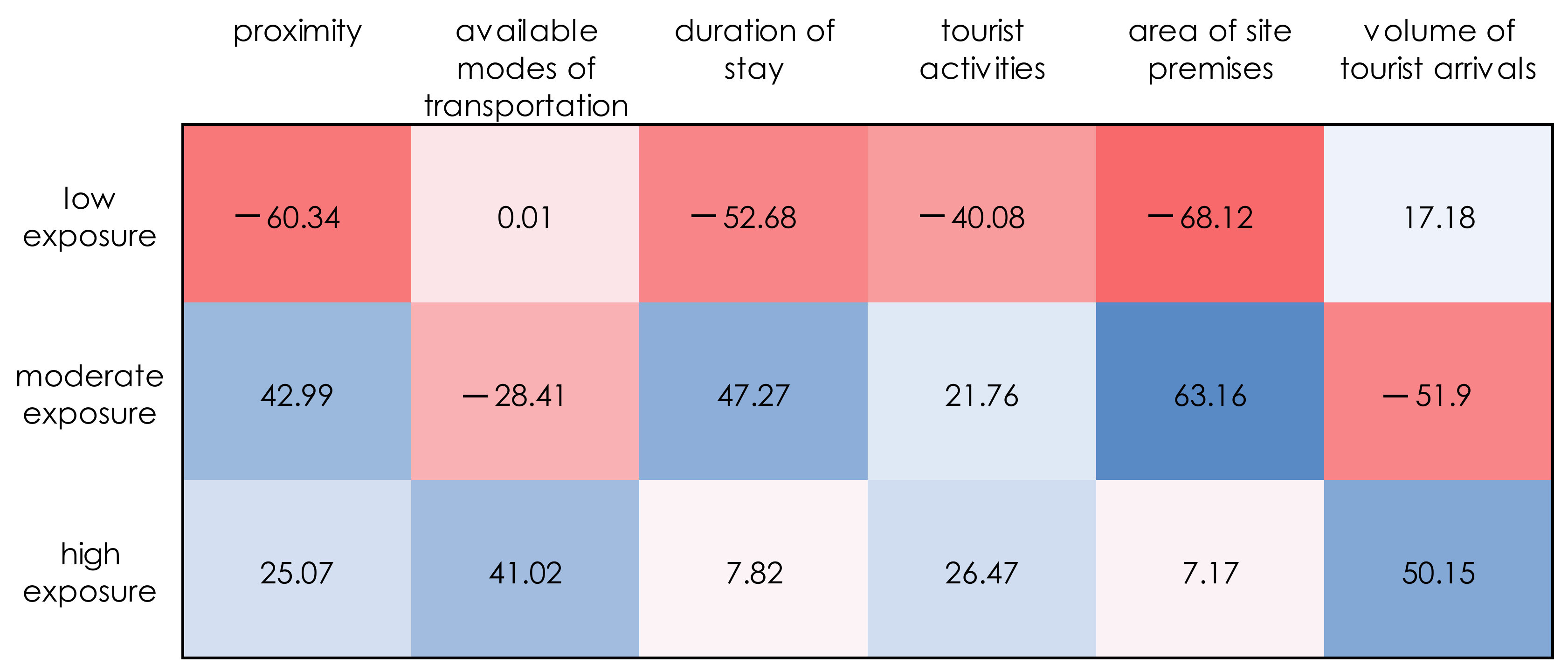
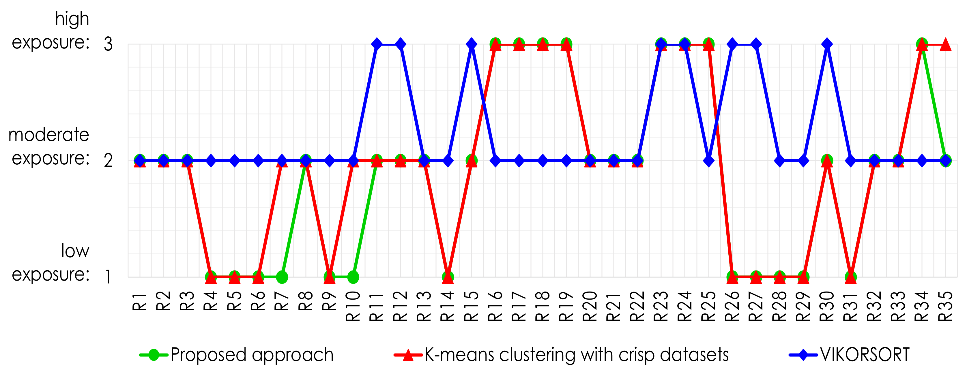
Case Study 1: Tourist Sites

In Figure 3, we compare the results of the proposed approach in Case study 1 with that of the VIKORSORT [3] and offer some insights. Using the proposed approach, the assignments yield 12, 15, and eight sites to “low exposure”, “moderate exposure”, and “high exposure” cluster, respectively. Note that these assignments vary significantly with the results of the VIKORSORT, with no site assigned to the “low exposure” cluster, 27 sites to “moderate exposure”, and eight sites to the “high exposure” cluster. Ten sites (i.e., S4, S5, S6, S7, S9, S10, S14, S28, S29, S31) from the “moderate exposure” cluster [3] were considered in the “low exposure” cluster with the proposed approach, while two sites (S26, S27) initially assigned by the VIKORSORT to the “high exposure” cluster are downgraded to “low exposure” cluster. These two sites belong to water-based tourism, and tourist arrivals are currently controlled via capacity restrictions of the government. All but three sites (i.e., S11, S12, S30) assigned to the “moderate exposure” cluster (proposed approach) are also assigned to the same cluster (VIKORSORT). While the area of these three sites is limited, tourist arrivals and duration of stay are minimum due to the limited activities available in these sites and the imposed limits on capacity by the government. Six sites (i.e., S16, S17, S18, S19, 25, 34) assigned to the “moderate exposure” cluster (VIKORSORT) are transferred to the “high exposure” cluster (proposed method). On the other hand, four sites (i.e., S11, S12, S15, S30) in the “high exposure” cluster (VIKORSORT) are downgraded to the “moderate exposure” cluster (proposed approach). When comparing the proposed approach with $k$-means clustering with the crisp dataset, minor differences can be observed. For instance, two sites (i.e., S7, S10) are assigned to the “low exposure” (proposed method) instead of “moderate exposure” (VIKORSORT). This assignment seems necessary as these two sites are beaches with low tourist arrivals; thus, physical distancing measures can be easily implemented. Lake Danao (S35) is assigned to the “high exposure” cluster (crisp $k$-means clustering), while this site has a low volume of tourist arrivals. Thus, the proposed method is plausible in assigning S35 to the “moderate exposure” cluster.

A more detailed analysis suggests that the sun, sea, sand sites have mostly downgraded from “moderate exposure” (VIKORSORT) to “low exposure” (proposed approach), except for Panagsama beach (S2) and Basdaku (S4). The two beach sites are considered top popular beach sites in the locality, in comparison with other beach sites (i.e., S7, S8, S9, S10), with their high volume of tourist arrivals and the jump-off point to various tourist activities (e.g., island tours, snorkeling, scuba diving). Thus, S2 and S4 are justifiably assigned at the “moderate exposure” cluster. Other sun, sea, sand sites are remote small island sites (e.g., S1, S5, S6) with proximity and area criteria affecting tourist choice. Hence, the proposed methods provide a reasonable assignment of these sites. Secondly, the heritage and culture sites have greatly differing assignments, from “moderate exposure” (VIKORSORT) to “high exposure” (proposed method), making all sites in this type assigned to the “high exposure” cluster. The proximity of these sites is overwhelmed with their enclosed environment, which increases the exposure of tourists to COVID-19. Third, ecotourism sites have mostly downgraded from “moderate exposure” (VIKORSORT) to “low exposure” (proposed approach). Ecotourism sites have been practicing social and environmental carrying capacity with their relatively low tourist arrivals, implying “low exposure” to COVID-19. Fourth, water-based sites have mostly been downgraded from high (VIKORSORT) to “moderate exposure” (proposed method). Water-based sites mainly limit the duration of stay of the tourists, most activities are undertaken in-group and by batches (i.e., family, friends), imposing carrying capacity, and the area is wide and open if not well ventilated. Water-based sites have already implemented proper monitoring and management before the pandemic due to stakeholders’ pressure to manage increasing tourist arrivals. Despite that, current government restrictions discouraged this type of tourist’s travel (e.g., travel age restriction, site closure). Lastly, park sites yield the same assignments (i.e., “moderate exposure”), except for Baluarte Park (S34) and Lake Danao (S35) that are situated in rural areas with limited tourist activities. Both approaches (i.e., VIKORSORT, proposed method) agree on farm tourism sites belonging to the “moderate exposure” cluster.

To illustrate further the performance of the proposed method with the VIKORSORT and $k$-means clustering with crisp datasets, we subscribe to the similarity ratio metric ($S_r$) introduced by Ghorabaee et al. [71]. Equation (28) illustrates such a metric:

$$S_r=\frac{{{\displaystyle \sum }}_{i=1}^m{w}_i\left(x_i,y_i\right)}{m}, x_i,y_i\in \left\{”\mathrm{low} \mathrm{exposure}”, “\mathrm{moderate} \mathrm{exposure}”, “\mathrm{high} \mathrm{exposure}”\right\}$$

(28)

where, $w_i\left(x_i,y_i\right)=\left\{\begin{array}{c}1\\ 0\end{array}\right.\begin{array}{c}\mathrm{if} x_i=y_i, \\ \mathrm{if} x_i\ne y_i,\end{array} .m$ denotes the number of alternatives (i.e., tourist sites), $x_i$ is the cluster of the $i$th alternative using the first method, and $y_i$ is the cluster of the $i$th alternative using the second method. As a consequence, full agreement of all assignments for any two methods implies yields $S_r=1$.

Table 16. Comparing the assignments of tourist sites to clusters with VIKORSORT, $k$-means clustering with crisp datasets, and the proposed approach based on $S_r$.

	Vikorsort	$\mathit{K}$-Means Clustering with Crisp Datasets	Proposed Approach
VIKORSORT	1	0.400	0.371
$k$-means clustering with crisp datasets	-	1	0.914
Proposed approach	-	-	1

provides the values of $S_r$. Table 16 reveals noticeable differences in the assignments between using the VIKORSORT [3] and the proposed approach, as implied by its low $S_r=0.371$. This is comparable with the $S_r$ value between the VIKORSORT and the crisp $k$-means clustering. However, the crisp $k$-means clustering and the proposed approach yield high similarity of assignments, having $S_r=0.914$. Nevertheless, the minor differences may become more profound at scale application. These findings imply that the $k$-means clustering algorithms offer an entirely different view with plausible results.

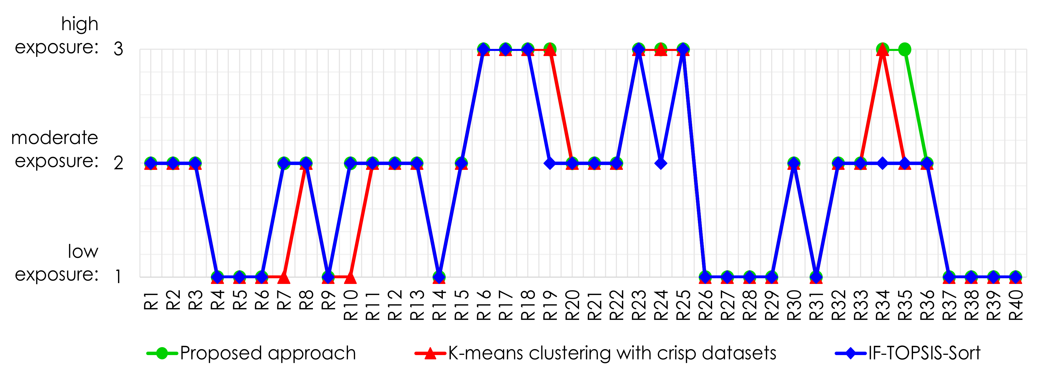
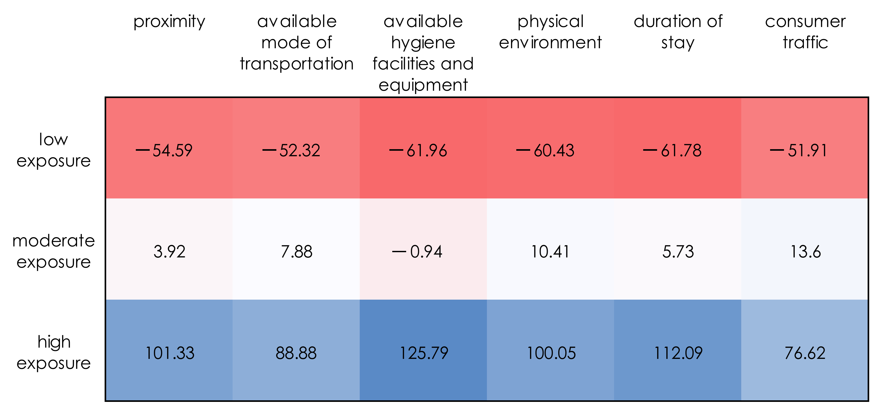
Case Study 2: Restaurants

The analysis employed for Case study 1 was carried out for Case study 2. In Figure 4, we compare the efficacy of the proposed approach in Case study 2 with that of the IF-TOPSIS-Sort carried out by Ocampo et al. [4] and offer some insights. Using the proposed approach, the assignments yield 14, 17, and 9 sites to “low exposure”, “moderate exposure”, and “high exposure” cluster, respectively. Note that these assignments do not vary a lot with the results of both the IF-TOPSIS-Sort and the $k$-means clustering with crisp datasets, which is apparent in

Table 17. Comparing the assignments of tourist sites to clusters with IF-TOPSIS-Sort, $k$ -means clustering with crisp datasets, and the proposed approach based on $S_r$.

	IF-TOPSIS-Sort	$\mathit{K}$-Means Clustering with Crisp Datasets	Proposed Approach
IF-TOPSIS-Sort	1	0.875	0.9
$k$-means clustering with crisp datasets	-	1	0.925
Proposed approach	-	-	1

based on $S_r$ metric. However, some slight differences among the approaches are observable. For instance, unlike the IF-TOPSIS-Sort and the proposed approach, which assigns Hukad (R8) and Choobi-choobi (R10) to the “moderate exposure” cluster, the $k$-means clustering with crisp datasets downgrades the assignment of these restaurants to the “low exposure” cluster.

On the other hand, while the proposed approach and $k$-means clustering with crisp datasets assign Matias BBQ (R22) and Chinese Ngohiong (R24) to the “high exposure” cluster, the IF-TOPSIS-Sort downgrades the assignment of these restaurants to the “moderate exposure” cluster. The IF-TOPSIS-Sort also downgrades the assignment of McDonald’s (R33) to the “moderate exposure” cluster while the other two approaches classify it in the “high exposure” cluster. The last difference observed is when the proposed approach appreciates the assignment of Orange Brutus (R36) to the “high exposure” cluster. At the same time, the other approaches classify it in the “moderate exposure” cluster. These inconsistencies in cluster assignment are considered relatively minimal, which is evident in the results wherein most of the assignments in one cluster are consistent with the other approaches. On the basis of these results, the proposed approach may, thus, be likened to both the IF-TOPSIS-Sort and $k$-means clustering with crisp datasets.

5.2. Sensitivity Analysis

A sensitivity analysis is carried out to evaluate the robustness of the proposed approach with minor changes in the model parameters (i.e., equivalent IVIFS values of the linguistic variables). Robustness is defined here as the tendency of the clustering results to resist change despite changes in key parameter values. The evaluation of robustness is critical as IVIFS values may be arbitrarily assigned to linguistic terms, which can alter inputs and, in turn, alter the results of the proposed clustering procedure. In performing the sensitivity analysis, the following conditions are set: Let $X=\left\{x_1,x_2,\dots ,x_n\right\}$ be the set of linguistic ratings in the scale where $x_1\prec x_2\prec \dots \prec x_n$. Note that the rating scale referred to here is the scale used to represent the linguistic variables used by the decision-makers (respondents) to elicit judgments. Also, let $M=\left\{m_1,m_2,\dots ,m_n\right\}$ be such that $m_1=0.5{\psi }_o$ and $m_i=m_{i-1}+d$, $\forall i\in \left\{2,\dots ,n\right\}$, where $d=\left(1-{\psi }_o\right){\left(n-1\right)}^{-1}$. Here, $M$ is the set of the centers of the interval membership degrees of the elements in $X$ assuming ${\mu }_{AL}^I\left(x_1\right)=0$ and ${\mu }_{AL}^I\left(x_n\right)=0.95$, while $d$ is the uniform distance of the centers from one another. The parameter $d$ ensures the uniform spacing of memberships of the ratings in the scale. Also, ${\psi }_o\in \left[0,1\right]$ is the parameter defining the “interval length” of the membership of $x$, hence ${\psi }_o={\mu }_{AU}^I\left(x\right)-{\mu }_{AL}^I\left(x\right)$, $\forall x\in X$. It is also assumed that ${\gamma }_{AL}^I\left(x\right)=0.5{\gamma }_{AU}^I\left(x\right)$ and ${\gamma }_{AU}^I\left(x\right)=1-{\mu }_{AU}^I\left(x\right)$, $\forall x\in X$. Finally, the following are introduced:

$${\mu }_{AL}^I\left(x_i\right)=m_i-\left(0.5{\psi }_o\right),\forall i\in \left\{1,2,\dots , n\right\}$$

(29)

$${\mu }_{AU}^I\left(x_i\right)=m_i+\left(0.5{\psi }_o\right),\forall i\in \left\{1,2,\dots , n\right\}$$

(30)

These conditions are set to establish a standard method for varying the IVIFS values through the parameter ${\psi }_o$. In this analysis, ${\psi }_o=\left\{0.15, 0.20, 0.25,0.30,0.35\right\}$ is used in both case studies to test how the results vary with different overlapping IVIFS values. Note that, in both cases, the original IVIFS values are not overlapping (see Table 2 and Table 8). The resulting IVIFS values corresponding to the five ${\psi }_o$ values are presented in

Table 18. Resulting IVIFS values for the case of assigning tourist sites.

Rating	${\mathit{\psi }}_{\mathit{o}}=\mathbf{0.15}$	${\mathit{\psi }}_{\mathit{o}}=\mathbf{0.20}$	${\mathit{\psi }}_{\mathit{o}}=\mathbf{0.25}$	${\mathit{\psi }}_{\mathit{o}}=\mathbf{0.30}$	${\mathit{\psi }}_{\mathit{o}}=\mathbf{0.35}$
1	[(0,0.15),(0.43,0.85)]	[(0,0.2),(0.4,0.8)]	[(0,0.25),(0.38,0.75)]	[(0,0.3),(0.35,0.7)]	[(0,0.35),(0.33,0.65)]
2	[(0.1,0.25),(0.38,0.75)]	[(0.09,0.29),(0.35,0.71)]	[(0.09,0.34),(0.33,0.66)]	[(0.08,0.38),(0.31,0.62)]	[(0.08,0.43),(0.29,0.58)]
3	[(0.2,0.35),(0.33,0.65)]	[(0.19,0.39),(0.31,0.61)]	[(0.18,0.43),(0.29,0.58)]	[(0.16,0.46),(0.27,0.54)]	[(0.15,0.5),(0.25,0.5)]
4	[(0.3,0.45),(0.28,0.55)]	[(0.28,0.48),(0.26,0.52)]	[(0.26,0.51),(0.24,0.49)]	[(0.24,0.54),(0.23,0.46)]	[(0.23,0.58),(0.21,0.43)]
5	[(0.4,0.55),(0.23,0.45)]	[(0.38,0.58),(0.21,0.43)]	[(0.35,0.6),(0.2,0.4)]	[(0.33,0.63),(0.19,0.38)]	[(0.3,0.65),(0.18,0.35)]
6	[(0.5,0.65),(0.18,0.35)]	[(0.47,0.67),(0.17,0.33)]	[(0.44,0.69),(0.16,0.31)]	[(0.41,0.71),(0.15,0.29)]	[(0.38,0.73),(0.14,0.28)]
7	[(0.6,0.75),(0.13,0.25)]	[(0.56,0.76),(0.12,0.24)]	[(0.53,0.78),(0.11,0.23)]	[(0.49,0.79),(0.11,0.21)]	[(0.45,0.8),(0.1,0.2)]
8	[(0.7,0.85),(0.08,0.15)]	[(0.66,0.86),(0.07,0.14)]	[(0.61,0.86),(0.07,0.14)]	[(0.57,0.87),(0.07,0.13)]	[(0.53,0.88),(0.06,0.13)]
9	[(0.8,0.95),(0.03,0.05)]	[(0.75,0.95),(0.03,0.05)]	[(0.7,0.95),(0.03,0.05)]	[(0.65,0.95),(0.03,0.05)]	[(0.6,0.95),(0.03,0.05)]

(for the assignment of tourist sites) and

Table 19. Resulting IVIFS values for the case of assigning restaurants.

Rating	${\mathit{\psi }}_{\mathit{o}}=\mathbf{0.15}$	${\mathit{\psi }}_{\mathit{o}}=\mathbf{0.20}$	${\mathit{\psi }}_{\mathit{o}}=\mathbf{0.25}$	${\mathit{\psi }}_{\mathit{o}}=\mathbf{0.30}$	${\mathit{\psi }}_{\mathit{o}}=\mathbf{0.35}$
1	[(0,0.15),(0.43,0.85)]	[(0,0.2),(0.4,0.8)]	[(0,0.25),(0.38,0.75)]	[(0,0.3),(0.35,0.7)]	[(0,0.35),(0.33,0.65)]
2	[(0.16,0.31),(0.35,0.69)]	[(0.15,0.35),(0.33,0.65)]	[(0.14,0.39),(0.31,0.61)]	[(0.13,0.43),(0.29,0.57)]	[(0.12,0.47),(0.27,0.53)]
3	[(0.32,0.47),(0.27,0.53)]	[(0.3,0.5),(0.25,0.5)]	[(0.28,0.53),(0.24,0.47)]	[(0.26,0.56),(0.22,0.44)]	[(0.24,0.59),(0.21,0.41)]
4	[(0.48,0.63),(0.19,0.37)]	[(0.45,0.65),(0.18,0.35)]	[(0.42,0.67),(0.17,0.33)]	[(0.39,0.69),(0.16,0.31)]	[(0.36,0.71),(0.15,0.29)]
5	[(0.64,0.79),(0.11,0.21)]	[(0.6,0.8),(0.1,0.2)]	[(0.56,0.81),(0.1,0.19)]	[(0.52,0.82),(0.09,0.18)]	[(0.48,0.83),(0.09,0.17)]
6	[(0.8,0.95),(0.03,0.05)]	[(0.75,0.95),(0.03,0.05)]	[(0.7,0.95),(0.03,0.05)]	[(0.65,0.95),(0.03,0.05)]	[(0.6,0.95),(0.03,0.05)]

(for the assignment of restaurants).

Three cluster performance metrics are used to evaluate the clustering performance of the proposed procedure for each value of ${\psi }_o$. First is the average within centroid distance (${\xi }_{cent}$). This metric pertains to the average distance of the observations (i.e., tourist sites, restaurants) to the cluster centroid. It measures the variability of the observations within each cluster. The next metric is the average within-cluster distance (${\xi }_{clust}$). This metric measures the cluster density performance, calculated using the average distance between points in a cluster, and multiplies this by the number of points minus one. Lastly, the Davies-Bouldin index (${\xi }_{DBI}$) is used to evaluate the goodness of split by the clustering procedure. The ${\xi }_{DBI}$ is calculated as the average similarity of each cluster with a cluster most similar to it. For all the metrics mentioned here, lower values suggest the better the clusters are separated and the better is the result of the clustering. The performance of the clustering procedure for the five values of the parameter ${\psi }_o$ is presented in

Table 20. Sensitivity analysis of the proposed method for the assignment of tourist sites.

${\mathit{\psi }}_{\mathit{o}}$	$\mathbf{Overall} {\mathit{\xi }}_{\mathit{c}\mathit{e}\mathit{n}\mathit{t}}$	$\mathbf{Low} \mathbf{Exposure}\text{:} {\mathit{\xi }}_{\mathit{c}\mathit{e}\mathit{n}\mathit{t}}$	$\mathbf{Moderate} \mathbf{Exposure}\text{:} {\mathit{\xi }}_{\mathit{c}\mathit{e}\mathit{n}\mathit{t}}$	$\mathbf{High} \mathbf{Exposure}: {\mathit{\xi }}_{\mathit{c}\mathit{e}\mathit{n}\mathit{t}}$	$\mathbf{Overall} {\mathit{\xi }}_{\mathit{c}\mathit{l}\mathit{u}\mathit{s}\mathit{t}}$	$\mathbf{Low} \mathbf{Exposure}: {\mathit{\xi }}_{\mathit{c}\mathit{l}\mathit{u}\mathit{s}\mathit{t}}$	$\mathbf{Moderate} \mathbf{Exposure}: {\mathit{\xi }}_{\mathit{c}\mathit{l}\mathit{u}\mathit{s}\mathit{t}}$	$\mathbf{High} \mathbf{Exposure}: {\mathit{\xi }}_{\mathit{c}\mathit{l}\mathit{u}\mathit{s}\mathit{t}}$	${\mathit{\xi }}_{\mathit{D}\mathit{B}\mathit{I}}$
0.15	0.004	0.002	0.002	0.006	0.862	0.734	0.438	1.283	0.767
0.20	0.003	0.002	0.001	0.006	0.806	0.684	0.408	1.203	0.765
0.25	0.003	0.002	0.001	0.005	0.750	0.634	0.379	1.123	0.763
0.30	0.002	0.001	0.001	0.004	0.694	0.584	0.351	1.042	0.761
0.35	0.002	0.001	0.001	0.004	0.639	0.535	0.322	0.961	0.760

(Case study 1) and

Table 21. Sensitivity analysis of the proposed method for the assignment of restaurants.

${\mathit{\psi }}_{\mathit{o}}$	$\mathbf{Overall} {\mathit{\xi }}_{\mathit{c}\mathit{e}\mathit{n}\mathit{t}}$	$\mathbf{Low} \mathbf{Exposure}: {\mathit{\xi }}_{\mathit{c}\mathit{e}\mathit{n}\mathit{t}}$	$\mathbf{Moderate} \mathbf{Exposure}: {\mathit{\xi }}_{\mathit{c}\mathit{e}\mathit{n}\mathit{t}}$	$\mathbf{High} \mathbf{Exposure}: {\mathit{\xi }}_{\mathit{c}\mathit{e}\mathit{n}\mathit{t}}$	$\mathbf{Overall} {\mathit{\xi }}_{\mathit{c}\mathit{l}\mathit{u}\mathit{s}\mathit{t}}$	$\mathbf{Low} \mathbf{Exposure}: {\mathit{\xi }}_{\mathit{c}\mathit{l}\mathit{u}\mathit{s}\mathit{t}}$	$\mathbf{Moderate} \mathbf{Exposure}: {\mathit{\xi }}_{\mathit{c}\mathit{l}\mathit{u}\mathit{s}\mathit{t}}$	$\mathbf{High} \mathbf{Exposure}: {\mathit{\xi }}_{\mathit{c}\mathit{l}\mathit{u}\mathit{s}\mathit{t}}$	${\mathit{\xi }}_{\mathit{D}\mathit{B}\mathit{I}}$
0.15	0.002	0.001	0.003	0.002	0.721	0.770	0.476	0.795	0.637
0.20	0.001	0.001	0.002	0.001	0.660	0.705	0.436	0.726	0.637
0.25	0.001	0.001	0.002	0.001	0.601	0.643	0.398	0.660	0.637
0.30	0.001	0.001	0.001	0.001	0.545	0.583	0.361	0.598	0.637
0.35	0.001	0.001	0.001	0.001	0.491	0.526	0.326	0.538	0.637

(Case study 2).

For both cases, the elements in each cluster for all values of ${\psi }_o$ are the same as the initial results of the case studies. This finding suggests that the proposed approach is robust to minor changes in the model parameters. Also, note that as the value of ${\psi }_o$ increases, the overlap of the interval membership functions of the ratings also increases for all cluster performance metrics considered in this work. Table 20 and Table 21 show a consistent improvement in the clustering performance of the proposed method as ${\psi }_o$ increases.

6. Discussion

The proposed approach offers insightful contributions to both practical and methodological aspects of $k$-means clustering. As demonstrated in this work, the agenda of categorizing the degree of exposure of tourists or customers to COVID-19, previously explored in our works [2,3,4], is crucial to the recovery of the tourism and hospitality sector despite the availability of vaccines. With the identified evaluation criteria for tourist site evaluation, the proposed approach yields the same priority ranking [3], which suggests that proximity with the top priority, followed by the volume of tourist arrivals, available modes of transportation, area of site premises, tourist activities, and duration of stay at the bottom of the list. Accordingly, authorities can set these insights as guidelines in developing measures that would promote sectoral recovery while curbing disease spread. Our previous works offered some plausible directions rooted in this ranking of criteria. On the other hand, evaluating the set of restaurants results in a different ranking of criteria associated with the exposure of customers to COVID-19. While proximity ranks on top for tourist sites, the same criterion has the least priority compared to other criteria. Instead, the availability of hygiene facilities and equipment emerges with the highest priority, followed by the physical environment, consumer traffic, available mode of transportation, and duration of stay. This implies that customers give a premium to the availability of hygiene facilities and equipment and the physical environment when dining in restaurants amidst the pandemic. This finding is almost straightforward, as COVID-19 spread is highly linked to the physical characteristics of the restaurants. Aside from these two attributes, customers are mindful of consumer traffic when dining in, indicating the importance of physical distancing measures. These top three attributes imply that customers put more emphasis on the characteristics of the restaurants themselves, not on the manner of getting into the location.

To initiate a comparison with the previous categorization, the proposed approach assumes three clusters for the $k$-means clustering of tourist sites. Distinct characteristics for each cluster are revealed. The “low exposure” cluster includes tourist sites with small premises, closer to home, with activities that allow tourists not to stay longer. The “moderate exposure” cluster, on the other hand, characterizes tourist sites with large premises where tourists can stay longer but with minimal tourist arrivals. Finally, the “high exposure” cluster involves sites with a huge volume of tourist arrivals that would engage in a higher number of tourist activities. Tourist arrivals in this cluster are encouraged by more available modes of transportation. These characterizations of clusters advance our previously reported findings [3], where multiple criteria sorting methods set these categories merely a priori by the analysts who might have limited knowledge of the domain problem. On the other hand, the proposed $k$-means clustering with IVIF datasets provides a practical approach by analyzing patterns within the dataset and reveals the shared characteristics of those tourist sites within the same cluster. Extracting these characteristics offers practical insights to tourists and tourism enterprises, as well as the government for policy- and decision-making. The proposed approach assigns 12 sites to the “low exposure” cluster, 15 sites to the “moderate exposure” cluster, and eight sites to the “high exposure cluster. While these assignments are idiosyncratic, meaningful insights that would associate the type of the tourist site and the cluster can be revealed to the case stakeholders and the general tourism sector.

Using the similar methodological framework adopted in the assignment of tourist sites, the evaluation of restaurants according to the perceived degree of exposure of customers to COVID-19 is demonstrated as a second case study. With $k=3$ set similarly, the “low exposure” cluster is characterized by restaurants that are just nearby, with low consumer traffic, and customers’ stay is shorter (e.g., food orders are served fast). The “moderate exposure” cluster contains restaurants that have an average rating on all evaluation criteria. That is, their evaluation scores lie on the average of all restaurants assessed in every criterion. Lastly, the “high exposure” cluster is associated with restaurants located at a distance, with high consumer traffic and longer service times (i.e., customers staying longer). Again, these characteristics that could not be gained from multiple criteria sorting methods are the major advantage of a clustering approach. In addition, the hospitality sector and the government would benefit from these characteristics as they would serve as guidelines for the post-pandemic recovery of the sector. On the other hand, customers can associate these characteristics of restaurants to other similar restaurants that are outside the evaluation reported in this work. This practical value is crucial to the recovery of the hospitality sector amidst the pandemic, with the emergence of variants that can escape vaccines. The proposed approach yields 16 restaurants assigned to the “low exposure” cluster, 16 labeled having “moderate exposure”, and eight in the “high exposure” cluster. Exploring the characteristics of these restaurants to assess other restaurants in other local regions is an added value.

Comparing with the multiple criteria sorting method (i.e., VIKORSORT) suggests that the results of the $k$-means clustering with IVIF datasets are more plausible as validated by the actual experiences of tourists in those sites under consideration. The proposed method yields better results; thus, it is preferable to use. This argument is motivated by the capability of the $k$-means clustering to extract patterns on the performance of each site on every criterion, as opposed to the predetermined identification of categories or clusters by the analysts who may have limited knowledge on the scope of the evaluation problem. Compared to the $k$-means clustering with crisp datasets, the proposed approach yields similar assignments 90% of the time for both cases. The minor difference in their assignments is associated with the integration of the IVIFS theory of $k$-means clustering, which better captures the vagueness and uncertainty of judgment elicitation of respondents. While the difference seems minor, its impact may become more profound when applied to a large-scale problem. Finally, by running a systematic sensitivity analysis, the proposed approach is robust to minor changes in the model parameters represented by the equivalent IVIFS values of the linguistic variables used in the evaluation process. On the other hand, comparing the proposed approach to that of the IF-TOPSIS-Sort by Ocampo et al. [4] yields minor differences, which is interesting because IF-TOPSIS-Sort does not abide by the principle of pattern extraction, which is the capability harnessed by the proposed approach. Nevertheless, these findings could indicate similarity between the proposed approach that incorporates IVIFs into the $k$-means clustering algorithm and the IF-TOPSIS-Sort, which may link pattern recognition approaches (i.e., $k$-means clustering) to MADM techniques (e.g., the TOPSIS method). Such an investigation is, however, beyond the scope of this work.

7. Conclusions and Future Works

The emergence of COVID-19 variants that can escape available vaccines further delays the full recovery of the tourism and hospitality sector. The fear of exposure to COVID-19 even among vaccinated individuals hinders tourists and customers in availing of the products and services offered by the sector. Thus, our prior works, which reported computational platforms of evaluating tourist sites (restaurants) according to the perceived exposure of tourists (customers) to COVID-19, remain a relevant approach to safe sectoral recovery and curb disease spread. However, the VIKORSORT, IF-TOPSIS-Sort, and other multiple-criteria sorting methods suffer from two major drawbacks. First, tourist sites and restaurants are assigned to predetermined categories defined by the analyst who may have limited knowledge of the problem domain. Secondly, the elicitation of judgments of the respondents (or decision-makers) fails to consider the vagueness and uncertainty brought about by the decision-makers lack of knowledge and experience or their limited information processing capabilities. Thus, this work advances these gaps by performing $k$-means clustering with IVIF datasets. The $k$-means clustering offers a more practical evaluation by extracting clusters based on the shared characteristics of the tourist sites; thus, eliminating the subjectivity of introducing pre-determined categories as in multi-criteria sorting methods (i.e., VIKORSORT, IF-TOPSIS-Sort). The integration of the IVIFS theory augments the limitation of $k$-means clustering in handling datasets with vague and imprecise observations, especially in application domains where observations represent human judgments. In addition, the proposed approach incorporates the weights of the attributes (or criteria), which are not addressed in traditional $k$-means clustering. This mechanism, an enhancement of $k$-means clustering, is particularly useful in evaluation problems where attributes have varying priorities.

To demonstrate the proposed approach, the same problem domain, reported elsewhere, of evaluating 35 tourist sites under six criteria elucidating the degree of exposure of tourists to COVID-19 is carried out in this work. Similarly, a second case study, also reported elsewhere, evaluates restaurants according to customers’ exposure to COVID-19. Results suggest that the priority ranking of criteria for evaluating tourist sites shares similarity with the previous findings: proximity emerges on top, followed by the volume of tourist arrivals, available modes of transportation, area of site premises, tourist activities, and duration of stay. This ranking seems in contrast with the priority ranking of criteria for evaluating restaurants, which indicates that customers emphasize the physical characteristics of the restaurants, such as the availability of hygiene facilities and equipment, physical environment, and consumer traffic. By fixing $k=3$ for both case studies, the proposed approach yields distinct characteristics of the three clusters, which can be associated with “low exposure”, “moderate exposure”, and “high exposure” of tourists to COVID-19. In the first case study, 12 sites, 15 sites, and eight sites are assigned to the “low exposure” cluster, “moderate exposure” cluster, and “high exposure” cluster, respectively. Although idiosyncrasies exist, the value of associating the type of the tourist site and its resulting cluster is crucial for establishing measures that could contribute to the sectoral recovery. Similarly, the proposed method provides distinct characteristics of the three clusters (i.e., “low exposure”, “moderate exposure”, and “high exposure”) where restaurants in the second case study are assigned to. Results reveal that 16 restaurants are assigned to “low exposure”, 16 to “moderate exposure”, and eight to “high exposure” clusters, respectively. Considering the characteristics of the clusters, customers may evaluate any restaurant according to their perceived exposure to COVID-19.

Finally, compared to the VIKORSORT and IF-TOPSIS-Sort, the proposed approach offers more verifiable and practical results, owing to the capability of the $k$-means clustering to extract patterns of the characteristics of the alternatives in establishing distinct clusters. These characteristics can provide better guidelines to tourists, customers, and authorities in the safe recovery of the tourism and hospitality sector. The proposed approach is also robust to small changes in the model parameters (i.e., equivalent IVIFS values in judgment elicitation). As opposed to $k$-means clustering with crisp datasets, integrating the IVIFS theory and the inclusion of criteria weights offers a promising approach for clustering problems with attributes having varying weights and with datasets represented by human judgments containing inherent vagueness and uncertainty. Future works could explore other possible applications of the proposed approach outside the tourism and hospitality sector. The use of the proposed approach for big datasets with non-sharp data is an interesting future direction. Other fuzzy set extensions such as type-2 fuzzy sets, intuitionistic fuzzy sets, neutrosophic sets, Pythagorean fuzzy sets, among others, could be used instead of IVIF sets.

References

1. Dryhurst, S.; Schneider, C.R.; Kerr, J.; Freeman, A.L.J.; Recchia, G.; van der Bles, A.M.; Spiegelhalter, D.; van der Linden, S. Risk perceptions of COVID-19 around the world. J. Risk Res. 2020, 23, 994–1006. [Google Scholar] [CrossRef]
2. Yamagishi, K.; Ocampo, L. Utilizing TOPSIS-Sort for sorting tourist sites for perceived COVID-19 exposure. Curr. Issues Tour. 2021, 1–11. [Google Scholar] [CrossRef]
3. Ocampo, L.; Yamagishi, K. Multiple criteria sorting of tourist sites for perceived COVID-19 exposure: The use of VIKORSORT. Kybernetes 2021. [Google Scholar] [CrossRef]
4. Ocampo, L.; Tanaid, R.A.; Tiu, A.M.; Selerio, E., Jr.; Yamagishi, K. Classifying the degree of exposure of customers to COVID-19 in the restaurant industry: A novel intuitionistic fuzzy set extension of the TOPSIS-Sort. Appl. Soft Comput. 2021, 113, 107906. [Google Scholar] [CrossRef]
5. Cong, L.; Ding, S.; Wang, L.; Zhang, A.; Jia, W. Image segmentation algorithm based on superpixel clustering. IET Image Process. 2018, 12, 2030–2035. [Google Scholar] [CrossRef]
6. Hossain, Z.; Akhtar, N.; Ahmad, R.; Rahman, M. A dynamic K-means clustering for data mining. Indones. J. Electr. Eng. Comput. Sci. 2019, 13, 521–526. [Google Scholar] [CrossRef]
7. Wen, L.; Zhou, K.; Yang, S. A shape-based clustering method for pattern recognition of residential electricity consumption. J. Clean. Prod. 2019, 212, 475–488. [Google Scholar] [CrossRef]
8. Shi, W.; Zeng, W. Application of k-means clustering to environmental risk zoning of the chemical industrial area. Front. Environ. Sci. Eng. 2014, 8, 117–127. [Google Scholar] [CrossRef]
9. Kuswandi, D.; Surahman, E.; Thaariq, Z.Z.A.; Muthmainnah, M. K-Means Clustering of Student Perceptions on Project-Based Learning Model Application. In Proceedings of the 2018 4th International Conference on Education and Technology (ICET), Malang, Indonesia, 26–28 October 2018; IEEE: Manhattan, NY, USA, 2018; pp. 9–12. [Google Scholar]
10. Khanmohammadi, S.; Adibeig, N.; Shanehbandy, S. An improved overlapping k-means clustering method for medical applications. Expert Syst. Appl. 2017, 67, 12–18. [Google Scholar] [CrossRef]
11. Pustokhina, I.V.; Pustokhin, D.A.; Rodrigues, J.J.P.C.; Gupta, D.; Khanna, A.; Shankar, K.; Seo, C.; Joshi, G.P. Automatic Vehicle License Plate Recognition Using Optimal K-Means with Convolutional Neural Network for Intelligent Transportation Systems. IEEE Access 2020, 8, 92907–92917. [Google Scholar] [CrossRef]
12. Rani, S.; Kholidah, K.N.; Huda, S.N. A Development of Travel Itinerary Planning Application using Traveling Salesman Problem and K-Means Clustering Approach. In Proceedings of the 2018 7th International Conference on Software and Computer Applications, Kuantan, Malaysia, 8–10 February 2018; ACM: New York, NY, USA, 2018; pp. 327–331. [Google Scholar]
13. Monica, S.; Natalia, F.; Sudirman, S. Clustering Tourism Object in Bali Province Using K-Means and X-Means Clustering Algorithm. In 2018 IEEE 20th International Conference on High Performance Computing and Communications; IEEE 16th International Conference on Smart City; IEEE 4th International Conference on Data Science and Systems (HPCC/SmartCity/DSS); IEEE: Manhattan, NY, USA, 2018; pp. 1462–1467. [Google Scholar]
14. Yang, H.; Luo, J.-D.; Fan, Y.; Zhu, L. Using weighted k-means to identify Chinese leading venture capital firms incorporating with centrality measures. Inf. Process. Manag. 2020, 57, 102083. [Google Scholar] [CrossRef]
15. Mahmoudi, A.; Deng, X.; Javed, S.A.; Yuan, J. Large-scale multiple criteria decision-making with missing values: Project selection through TOPSIS-OPA. J. Ambient. Intell. Humaniz. Comput. 2021, 12, 9341–9362. [Google Scholar] [CrossRef]
16. Park, J.H.; Park, I.Y.; Kwun, Y.C.; Tan, X. Extension of the TOPSIS method for decision making problems under interval-valued intuitionistic fuzzy environment. Appl. Math. Model. 2011, 35, 2544–2556. [Google Scholar] [CrossRef]
17. Zadeh, L.A. Fuzzy sets. Inf. Control. 1965, 3, 338–353. [Google Scholar] [CrossRef] [Green Version]
18. Atanassov, K.T. Intuitionistic fuzzy sets. Fuzzy Sets Syst. 1986, 20, 87–96. [Google Scholar] [CrossRef]
19. Ngan, R.T.; Son, L.H.; Ali, M.; Tamir, D.E.; Rishe, N.D.; Kandel, A. Representing complex intuitionistic fuzzy set by quaternion numbers and applications to decision making. Appl. Soft Comput. 2020, 87, 105961. [Google Scholar] [CrossRef]
20. Atanassov, K.; Gargov, G. Interval valued intuitionistic fuzzy sets. Fuzzy Sets Syst. 1989, 31, 343–349. [Google Scholar] [CrossRef]
21. Hu, K.; Tan, Q.; Zhang, T.; Wang, S. Assessing technology portfolios of clean energy-driven desalination-irrigation systems with interval-valued intuitionistic fuzzy sets. Renew. Sustain. Energy Rev. 2020, 132, 109950. [Google Scholar] [CrossRef]
22. Luo, M.; Liang, J. A Novel Similarity Measure for Interval-Valued Intuitionistic Fuzzy Sets and Its Applications. Symmetry 2018, 10, 441. [Google Scholar] [CrossRef] [Green Version]
23. Ananthi, V.; Balasubramaniam, P. A new image denoising method using interval-valued intuitionistic fuzzy sets for the removal of impulse noise. Signal. Process. 2016, 121, 81–93. [Google Scholar] [CrossRef]
24. Oztaysi, B.; Onar, S.C.; Kahraman, C.; Yavuz, M. Multi-criteria alternative-fuel technology selection using interval-valued intuitionistic fuzzy sets. Transp. Res. Part D Transp. Environ. 2017, 53, 128–148. [Google Scholar] [CrossRef]
25. Wu, L.; Wei, G.; Gao, H.; Wei, Y. Some Interval-Valued Intuitionistic Fuzzy Dombi Hamy Mean Operators and Their Application for Evaluating the Elderly Tourism Service Quality in Tourism Destination. Mathematics 2018, 6, 294. [Google Scholar] [CrossRef] [Green Version]
26. Cheng, S.-H. Autocratic multiattribute group decision making for hotel location selection based on interval-valued intuitionistic fuzzy sets. Inf. Sci. 2018, 427, 77–87. [Google Scholar] [CrossRef]
27. Kaur, S.P.; Gupta, V. COVID-19 Vaccine: A comprehensive status report. Virus Res. 2020, 288, 198114. [Google Scholar] [CrossRef]
28. Abu Bakar, N.; Rosbi, S. Effect of Coronavirus disease (COVID-19) to tourism industry. Int. J. Adv. Eng. Res. Sci. 2020, 7, 189–193. [Google Scholar] [CrossRef] [Green Version]
29. John Hopkins Coronavirus Resource Center. COVID-19 Dashboard by the Center for Systems Science and Engineering (CSSE) at Johns Hopkins University (JHU). Available online: https://coronavirus.jhu.edu/map.html (accessed on 31 July 2021).
30. Davahli, M.R.; Karwowski, W.; Sonmez, S.; Apostolopoulos, Y. The Hospitality Industry in the Face of the COVID-19 Pandemic: Current Topics and Research Methods. Int. J. Environ. Res. Public Health 2020, 17, 7366. [Google Scholar] [CrossRef]
31. Organization for Economic Co-Operation and Development. Tourism Policy Responses to Coronavirus (COVID-19). 2020. Available online: https://www.oecd.org/coronavirus/policy-responses/tourism-policy-responses-to-the-coronavirus-covid-19-6466aa20/ (accessed on 2 August 2021).
32. World Travel & Tourism Council (WTTC). Economic Impact Reports. World Travel & Tourism Council. 2021. Available online: https://wttc.org/Research/Economic-Impact (accessed on 30 July 2021).
33. Zhang, H.; Cho, T.; Wang, H. The Impact of a Terminal High Altitude Area Defense Incident on Tourism Risk Perception and Attitude Change of Chinese Tourists Traveling to South Korea. Sustainability 2020, 12, 7. [Google Scholar] [CrossRef] [Green Version]
34. Philippine Statistics Authority. Share of Tourism to GDP is 5.4 Percent in 2020. 2021. Available online: https://psa.gov.ph/tourism/satellite-accounts/id/164617 (accessed on 27 July 2021).
35. Asian Development Bank. The COVID-19 Impact on Philippine Business. June 2020. Available online: https://www.adb.org/sites/default/files/publication/622161/covid-19-impact-philippine-business-enterprise-survey.pdf (accessed on 25 July 2021).
36. Philippine Statistics Authority. Philippine GDP Posts -8.3 Percent in the Fourth Quarter 2020; -9.5 Percent for Full-Year 2020. Available online: https://psa.gov.ph/content/philippine-gdp-posts-83-percent-fourth-quarter-2020-95-percent-full-year-2020 (accessed on 28 January 2021).
37. Philippine Statistics Authority. Employed Persons by Sector, Subsector, and Hours Worked, Philippines. 2021. Available online: https://psa.gov.ph/system/files/Table%202-Employed%20Persons%20by%20Sector%2C%20Sub-sector%20and%20Hours%20Worked%2C%20Philippines%2C%20February%202021%2C%20March%202021%2C%20April%202021%20and%20May%202021_0.xlsx (accessed on 26 July 2021).
38. Kaushal, V.; Srivastava, S. Hospitality and tourism industry amid COVID-19 pandemic: Perspectives on challenges and learnings from India. Int. J. Hosp. Manag. 2021, 92, 102707. [Google Scholar] [CrossRef] [PubMed]
39. Dube, K.; Nhamo, G.; Chikodzi, D. COVID-19 cripples global restaurant and hospitality industry. Curr. Issues Tour. 2021, 24, 1487–1490. [Google Scholar] [CrossRef]
40. United Nations World Tourism Organization (UNWTO). UNWTO Launches a Call for Action for Tourism’s COVID-19 Mitigation and Recovery. 2020. Available online: https://www.unwto.org/news/unwto-launches-a-call-for-action-for-tourisms-covid-19-mitigation-and-recovery (accessed on 30 July 2021).
41. World Health Organization. WHO Coronavirus (COVID-19) Dashboard. Available online: https://covid19.who.int/ (accessed on 28 July 2021).
42. Gursoy, D.; Can, A.S.; Williams, N.; Ekinci, Y. Evolving impacts of COVID-19 vaccination intentions on travel intentions. Serv. Ind. J. 2021, 41, 719–733. [Google Scholar] [CrossRef]
43. Buhat, C.A.H.; Duero, J.C.C.; Felix, F.O.; Rabajante, J.F.; Mamplata, J.B. Optimal Allocation of COVID-19 Test Kits Among Accredited Testing Centers in the Philippines. J. Heal. Inform. Res. 2021, 5, 54–69. [Google Scholar] [CrossRef]
44. Gursoy, D.; Chi, C.G.; Chi, O.H. Effects of COVID 19 pandemic on restaurant and hotel customers’ sentiments towards dining out, traveling to a destination and staying at hotels. J. Hosp. 2021, 3, 1–17. [Google Scholar]
45. Hafeez, S.; Din, M.; Zia, F.; Ali, M.; Shinwari, Z.K. Emerging concerns regarding COVID-19; second wave and new variant. J. Med. Virol. 2021, 93, 4108. [Google Scholar] [CrossRef] [PubMed]
46. Padhi, A.K.; Tripathi, T. Can SARS-CoV-2 accumulate mutations in the S-protein to increase pathogenicity? ACS Pharmacol. Transl. Sci. 2020, 3, 1023–1026. [Google Scholar] [CrossRef] [PubMed]
47. Šostaks, A. Mathematics in the context of fuzzy sets: Basic ideas, concepts, and some remarks on the history and recent trends of development. Math. Model. Anal. 2011, 16, 173–198. [Google Scholar] [CrossRef]
48. Atanassov, K.T. Interval valued intuitionistic fuzzy sets. In Intuitionistic Fuzzy Sets; Physical: Heidelberg, Germany, 1999; pp. 139–177. [Google Scholar]
49. Xu, Z. Methods for aggregating interval-valued intuitionistic fuzzy information and their application to decision making. Control. Decis. 2007, 22, 215–219. [Google Scholar]
50. Xu, Z. A method based on distance measure for interval-valued intuitionistic fuzzy group decision making. Inf. Sci. 2010, 180, 181–190. [Google Scholar] [CrossRef]
51. Xu, Z.; Chen, J. Approach to group decision making based on interval-valued intuitionistic judgment matrices. Syst. Eng. Theory Pract. 2007, 27, 126–133. [Google Scholar] [CrossRef]
52. Ye, J. Multicriteria fuzzy decision-making method based on a novel accuracy function under interval-valued intuitionistic fuzzy environment. Expert Syst. Appl. 2009, 36, 6899–6902. [Google Scholar] [CrossRef]
53. Nayagam, V.L.G.; Muralikrishnan, S.; Sivaraman, G. Multi-criteria decision-making method based on interval-valued intuitionistic fuzzy sets. Expert Syst. Appl. 2011, 38, 1464–1467. [Google Scholar] [CrossRef]
54. Abualigah, L.M.; Khader, A.T.; Hanandeh, E.S. Hybrid clustering analysis using improved krill herd algorithm. Appl. Intell. 2018, 48, 4047–4071. [Google Scholar] [CrossRef]
55. Janani, R.; Vijayarani, S. Text document clustering using Spectral Clustering algorithm with Particle Swarm Optimization. Expert Syst. Appl. 2019, 134, 192–200. [Google Scholar] [CrossRef]
56. Ramirez, A.; Himang, C.; Selerio, E.; Manalastas, R.; Himang, M.; Giango, W.; Tenerife, P.; Ocampo, L. Exploring the Hedonic and Eudaimonic Motivations of Teachers for Pursuing Graduate Studies. Asia-Pac. Educ. Res. 2020. [Google Scholar] [CrossRef]
57. Selerio, E.F.; Arcadio, R.D.; Medio, G.J.; Natad, J.R.P.; Pedregosa, G.A. On the complex causal relationship of barriers to sustainable urban water management: A fuzzy multi-criteria analysis. Urban. Water J. 2021, 18, 12–24. [Google Scholar] [CrossRef]
58. Anitha, P.; Patil, M.M. RFM model for customer purchase behavior using K-Means algorithm. J. King Saud Univ. Comput. Inf. Sci. 2019, in press. [Google Scholar] [CrossRef]
59. Taheri, H.; Koester, L.W.; Bigelow, T.A.; Faierson, E.J.; Bond, L.J. In Situ Additive Manufacturing Process Monitoring with an Acoustic Technique: Clustering Performance Evaluation Using K-Means Algorithm. J. Manuf. Sci. Eng. 2019, 141, 1–27. [Google Scholar] [CrossRef]
60. Galvis, I.S.; Villa, Y.; Duarte, C.; Sierra, D.; Agudelo, W. Seismic attribute selection and clustering to detect and classify surface waves in multicomponent seismic data by using k-means algorithm. Lead. Edge 2017, 36, 239–248. [Google Scholar] [CrossRef]
61. Ramalingam, M.; Thangarajan, R. Mutated k-means algorithm for dynamic clustering to perform effective and intelligent broadcasting in medical surveillance using selective reliable broadcast protocol in VANET. Comput. Commun. 2020, 150, 563–568. [Google Scholar] [CrossRef]
62. Lloyd, S. Least squares quantization in PCM. IEEE Trans. Inf. Theory 1982, 28, 129–137. [Google Scholar] [CrossRef]
63. Forgy, E. Cluster analysis of multivariate data: Efficiency versus interpretability of classifications. Biometrics 1965, 21, 768–769. [Google Scholar]
64. Ocampo, L.; Yamagishi, K. Modeling the lockdown relaxation protocols of the Philippine government in response to the COVID-19 pandemic: An intuitionistic fuzzy DEMATEL analysis. Socio-Econ. Plan. Sci. 2020, 72, 100911. [Google Scholar] [CrossRef] [PubMed]
65. Department of Tourism DOT Pushes Stringent Guidelines for Stakeholders across the Nation. 2020. Available online: http://tourism.gov.ph/news_features/GuidelinesForStakeholders.aspx (accessed on 20 July 2021).
66. Department of Tourism DOT Statement on Uniform Travel Protocols. 2021. Available online: http://www.tourism.gov.ph/news_features/UniformTravelProtocols.aspx (accessed on 20 July 2021).
67. Rocamora, J.A.; Vaccination Key to Tourism Recovery. Philippine News Agency. 2021. Available online: https://www.pna.gov.ph/articles/1144200 (accessed on 31 July 2021).
68. Prosser, L.A.; Lavelle, T.A.; Fiore, A.E.; Bridges, C.B.; Reed, C.; Jain, S.; Dunham, K.M.; Meltzer, M.I. Cost-Effectiveness of 2009 Pandemic Influenza A(H1N1) Vaccination in the United States. PLoS ONE 2011, 6, e22308. [Google Scholar] [CrossRef] [PubMed] [Green Version]
69. Asian Development Bank. (28 April 2021). Philippine Economy Seen Recovering in 2021, with Stronger Growth in 2022—ADB. Available online: https://www.adb.org/news/philippine-economy-seen-recovering-2021-stronger-growth-2022-adb (accessed on 29 July 2021).
70. Markowitz, A. State-by-State Guide to Face Mask Requirements. AARP. Available online: https://www.aarp.org/health/healthy-living/info-2020/states-mask-mandates-coronavirus.html (accessed on 10 February 2021).
71. Ghorabaee, M.K.; Zavadskas, E.K.; Olfat, L.; Turskis, Z. Multi-Criteria Inventory Classification Using a New Method of Evaluation Based on Distance from Average Solution (EDAS). Informatica 2015, 26, 435–451. [Google Scholar] [CrossRef]
Figure 1. Differentiators (%) of the three clusters of tourist sites based on average.
Mathematics 09 02639 g001
Figure 2. Differentiators (%) of the three clusters of restaurants based on average.
Mathematics 09 02639 g002
Figure 3. Assignments of tourist sites to clusters with VIKORSORT, k -means clustering with crisp datasets, and the proposed approach.
Mathematics 09 02639 g003
Figure 4. Assignments of tourist sites to clusters with IF-TOPSIS-Sort, k -means clustering with crisp datasets, and the proposed approach.
Mathematics 09 02639 g004