Algorithmic Analysis of Finite-Source Multi-Server Heterogeneous Queueing Systems

Abstract

The paper deals with a finite-source queueing system serving one class of customers and consisting of heterogeneous servers with unequal service intensities and of one common queue. The main model has a non-preemptive service when the customer can not change the server during its service time. The optimal allocation problem is formulated as a Markov-decision one. We show numerically that the optimal policy which minimizes the long-run average number of customers in the system has a threshold structure. We derive the matrix expressions for performance measures of the system and compare the main model with alternative simplified queuing systems which are analysed for the arbitrary number of servers. We observe that the preemptive heterogeneous model operating under a threshold policy is a good approximation for the main model by calculating the mean number of customers in the system. Moreover, using the preemptive and non-preemptive queueing models with the faster server first policy the lower and upper bounds are calculated for this mean value.

1. Introduction

The finite-source or finite-population queueing systems comparing to the ordinary markovian queues have no longer a Poisson arrival stream as in systems with an infinite source of customers, but rather have a finite source capacity N of possible customers. In such systems a customer can be inside the system, consisting in our case of one common queue with capacity N and K heterogeneous servers or outside the system in so-called arriving state. It is assumed that each customer outside arrives to the system in exponentially distributed time. After receiving the service a customer returns to the arriving area. Much attention by the study of finite-source queueing systems has been paid in terms of the machine repairman problem, see e.g., [1,2]. The customers outside the queueing system can be interpreted as unreliable machines with independent exponentially distributed life times. The queueing system represents then the repair facility where the failed machines must be recovered. Such systems are also used in various dispatching problems, they are appropriate queueing models for telephone registration systems, call centers, Ethernet systems, local-area networks, mobile communications, magnetic disk memory systems and so on.

The primary objective of this paper is to analyze optimal control and to evaluate performance metrics under fixed control policy for a non-preemptive finite-source queueing system with one class of customers and heterogeneous servers. In such a system, a customer that receives service on a slower server cannot change it if a faster server becomes available in the course of service. Unfortunately, performance analysis of this system in analytical form is limited firstly by the need to have a known allocation mechanism between the servers or control policy and secondly by the dimensionality of the corresponding Markov process, which is affected by the number of servers. To calculate the optimal allocation policy with the aim to minimize the long-run average number of customers in the system we formulate the Markov decision process (MDP) and apply the policy-iteration algorithm. This algorithm can be used not only for the optimal allocation policy calculation but also to obtain the mean number of customers in the system operating under that policy. Numerical experiments confirm our expectations that the optimal policy is of threshold type as in the models with an infinite source capacity [3]. According to this policy the fastest server must be activated whenever there is a customer in the system while the slower servers must be used only if the number of customers in the queue reaches some prespecified threshold level. The model of the non-preemptive queue operating under the optimal threshold policy (OTP) will referred to in the paper as the OTP-model.

The task of calculating other system performance characteristics for a given control policy remains unresolved. Furthermore, it should be taken into account that despite of advantages the policy-iteration algorithm has a limitation on the dimensionality of the random process for an arbitrary number of servers. In case of a threshold control policy for a particular states’ ordering the corresponding Markov chain is a quasi-birth-and-death (QBD) process with a three-diagonal block infinitesimal matrix, where the blocks depend on the values of thresholds as it was shown in [4] for the infinite population system. In this case, matrix-analytic solution methods can be applied, but for a limited number of servers. This led us to discuss here in addition some simplified variants of the main model. The non-preemptive queueing system operating under a Fastest Server First (FSF) policy which prescribes for service the usage of the fastest idle server in each state and the preemptive queueing system (PS), where the service in a slower server can be interrupted if during the service time the faster server becomes idle. This system will operates according to a threshold policy, when the slower servers are activated or deactivated if the number of customers in the queue respectively exceeds or falls below a certain threshold level. Although these systems are simpler than the main model and have a low dimensions of the state-space, there are very few publications on such specific systems, especially those with analytical results.

Description of standard finite-source models with classical results, motivation examples and literature overview can be found in [5]. In [6] the author obtained the product form solution for the stationary state distribution for the finite population queueing model with a queue-dependent servers. A non-preemptive finite-population queueing system with heterogeneous classes of customers and a single server was studied in [7]. The problem of the throughput maximizing in a finite-source system with parallel queues was analyzed in [8], where some structural properties of the optimal control policy was proved. Heterogeneous multi-server finite-source queues with a FSF-policy and retrial phenomenon have been studied in [9], where numerical results were carried out by the help of the MOSEL tool. The model with machines having non-identical exponential service times was analysed in [10], where the repair policies which minimize the mean processing cost were considered. As for finite-source systems operating under a threshold policy, we know only research papers dedicated to single server systems with a unit threshold N-policy, see e.g., [11]. Here the threshold policy states that the server in a repair facility must be switched on only when the number of failed machines reaches to predefined threshold level N. In [12], the authors generalized the model to the case of two heterogeneous unreliable servers operating under policies $N_1$ and $N_2$. Although there is a considerable amount of results on finite-source queues, the controlled systems with heterogeneous servers operating without preemption have not been investigated before. Therefore, the models presented in this paper and the corresponding results of the system analysis differ from those previously discussed.

The main contributions of paper are as follows. The structural or threshold properties of an optimal control policy are numerically established. We derive for the main model the matrix expressions used further by calculating different performance measures such as the mean number of waiting customers, the mean number of busy servers, the mean length of a busy period. The matrix-analytic solution for the stationary state distribution and performance measures are obtained for the FSF-model. Here we used the recursive definition of some blocks in the infinitesimal matrix. For the PS-models we obtain analytical product-form result for an arbitrary number of servers. Moreover, it is shown that performance characteristics of these systems in certain operation modes are the same or very close to those of the main system functioning under the optimal policy. Thus, these simplified models can be used under certain conditions to calculate upper and lower bounds for some performance characteristics and also as approximating models. We develop also the first step analysis to study the mean number of customers served in the system or by the kth server in a busy period and the probability of the maximum queue length observed during this period.

The rest of the paper is organized as follows. In Section 2, we describe the Markov-decision process of the main model and show that the system has a threshold-based optimal allocation policy. In this section we develop also the computational analysis for the mean values of performance measures including those characterizing the behaviour of the system in a busy period. The FSF-Model is presented and analysed in Section 3. Section 4 is devoted to the PS-model. Comparison analysis of the proposed models and illustrative examples are summarized in Section 5.

The following notations will be used throughout this paper: $\mathbf{e}\left(n\right)$, ${\mathbf{e}}_j\left(n\right)$ and $I_n$ stand respectively for the unit vector of dimension n, for the basis vector of dimension n in ${\mathbb{R}}^n$ with $0\le j\le n-1$ or $1\le j\le n$ depending on the context, and for the identity matrix of dimension n. If it is not necessary to specify a vector dimension, we will omit the corresponding argument. For example, $\mathbf{e}$ denotes a column unit vector of an appropriate dimension. The notation ${}^{\prime }$ is used for the transpose. The notation ⊗ stands for the Kronecker product of two matrices, $1_{\left\{A\right\}}$ – for the indicator function, where $1_{\left\{A\right\}}=1$ if the condition A holds, and 0 otherwise. The notation $\left|A\right|$ is used for the magnitude of a finite set A.

2. OTP-Model

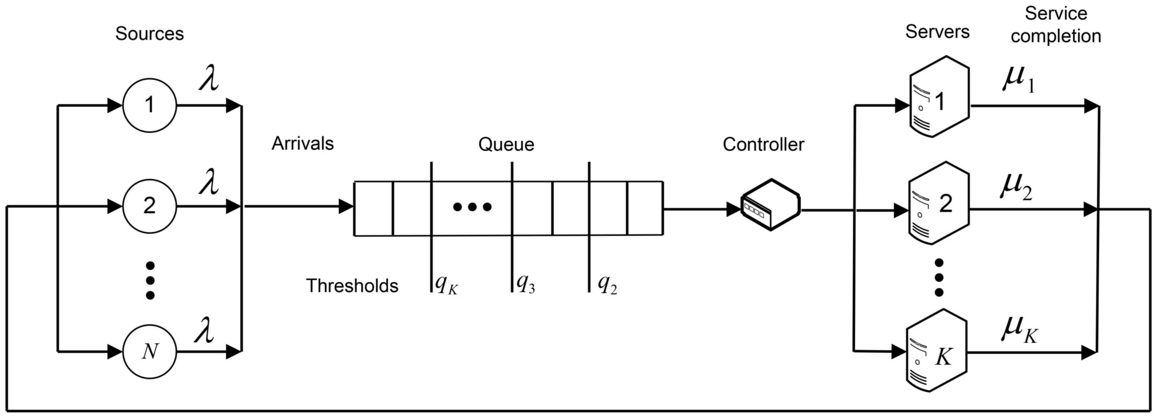
Here we discuss the main model of the non-preemptive finite-source controlled queueing system of the type $M/M/K/N//N$ illustrated in Figure 1. The system has K heterogeneous servers with different rates ${\mu }_1\ge {\mu }_2\ge \cdots \ge {\mu }_K>0$ and N customers in a source. It operates under the optimal allocation policy which minimizes the mean number of customers in the system. It will be shown that this policy is defined through a sequence of threshold levels $1=q_1\le q_2\le \cdots \le q_K<\infty$ for the queue lengths which prescribe the activation of slower servers. The analysed system can be treated as a model for the machine-repairman problem, where N unreliable machines in a working area with exponential distributed life times and equal rates $\lambda >0$ must be repaired by K heterogeneous repair stations. The machines fail independently of each other. The stream of failed machines can be treated as an arrival stream of customers to the queueing system. Hereafter, we will refer to the customer as a failed machine which enters the repair system and gets there a repair service. After the repair the machine becomes as good as a new one and it returns to the working area. The aim is to dynamically allocate the customers to the servers in order to minimize the long-run average number of customers in the system and to calculate the corresponding mean performance measures.

2.1. MDP Formulation

We formulate the optimal allocation problem in this machine-repairman system as a Markov Decision Process (MDP) in the following way. The behaviour of the system is described by a multi-dimensional continuous-time Markov-chain

$$\begin{array}{c}\hfill {\left\{X\left(t\right)\right\}}_{t\ge 0}={\{Q\left(t\right),D_1\left(t\right),\cdots ,D_K\left(t\right)\}}_{t\ge 0},\end{array}$$

(1)

where $Q\left(t\right)$ stands for the number of customers waiting in the queue at time t and $D_j\left(t\right)$ specifies the state of the jth server at time t, where

$$D_j\left(t\right)=\left\{\begin{array}{cc}0\hfill & \mathrm{if}\mathrm{the}\mathrm{server}j\mathrm{is}\mathrm{idle}\hfill \\ 1\hfill & \mathrm{if}\mathrm{the}\mathrm{server}j\mathrm{is}\mathrm{busy}.\hfill \end{array}\right.$$

State space: The set $E_X$ consists of $K+1$ dimensional row vectors,

$$\begin{array}{cc}\hfill E_X=& \{x=(q\left(x\right),d_1\left(x\right),\cdots ,d_K\left(x\right)):\hfill \\ \hfill & q\left(x\right)\in \{0,1,2,\cdots ,N-\sum _{j=1}^K{d}_j\left(x\right)\},d_j\left(x\right)\in \{0,1\},j=1,\cdots ,K\},\hfill \end{array}$$

where $q\left(x\right)$ denotes the number of customers in the queue and $d_j\left(x\right)$ – the status of the jth server in state x. The total number of states in the set $E_X$ is equal to $|E_X|={\sum }_{j=0}^K\left(\genfrac{}{}{0pt}{}{K}{j}\right)(N-j+1)$.

Decision epochs: The arrival and service completion epochs in the system with waiting customers.

Action space:$A=\{0,1,\cdots ,K\}$. To identify the group of idle and busy servers, the following sets are defined,

$$\begin{array}{c}\hfill J_0\left(x\right)=\{j:d_j\left(x\right)=0\},J_1\left(x\right)=\{j:d_j\left(x\right)=1\}.\end{array}$$

With this notations the set of admissible control actions $A\left(x\right)\subseteq A$ in state $x\in E_X$ can be defined as $A\left(x\right)=J_0\left(x\right)\cup \left\{0\right\}$. The action $a\in J_0\left(x\right)$ means that in state x a customer must be allocated to an idle server, while $a=0$ means that the customer must be routed to the queue. At an arrival epoch, which occurs only if the number of customers in the system is less than N, the arrived customer joins the queue and simultaneously another one from the head of the queue must be routed to some idle server or returned back to the queue. At a service completion epoch the same happens, i.e. the customer from the head of the queue is routed either to one of idle servers or to the queue again. By service completion in a system without waiting customers no actions have to be performed.

Immediate cost: The function $l\left(x\right)$ specifies the number of customers in a state $x\in E_X$, i.e.,

$$l\left(x\right)=q\left(x\right)+\sum _{j=1}^K{d}_j\left(x\right),$$

which is in fact independent of a control action a.

Transition rates: The policy-dependent infinitesimal matrix ${\Lambda }^f={\left[{\lambda }_{xy}\left(a\right)\right]}_{x,y\in E_X}$ of the Markov-chain (1) includes the rates to go from state x to state y given the control action is a defined as

$$\begin{array}{c}\hfill {\lambda }_{xy}\left(a\right)=\left\{\begin{array}{cc}(N-l(x\left)\right)\lambda \hfill & y=S_{a}x,0\le l\left(x\right)\le N,a\in A\left(x\right),\hfill \\ {\mu }_j\hfill & y=S_j^{-1}x,j\in J_1\left(x\right),q\left(x\right)=0,\hfill \\ {\mu }_j\hfill & y=S_0^{-1}{S}_j^{-1}{S}_{a}x,j\in J_1\left(x\right),q\left(x\right)>0,a\in A\left(S_0^{-1}{S}_j^{-1}x\right),\hfill \\ -\left(\right(N-l\left(x\right))\hfill & +\sum _{j\in J_1\left(x\right)}{\mu }_j)y=x,\hfill \\ 0\hfill & \mathrm{otherwise}\hfill \end{array}\right.\end{array}$$

(2)

with ${\lambda }_x\left(a\right)=-{\lambda }_{xx}\left(a\right)=-{\sum }_{y\ne x}{\lambda }_{xy}\left(a\right)$, where $S_a$ and $S_j^{-1}$ stand for the shift operators applied to the vector state x in the following way,

$$S_{a}x=x+{\mathbf{e}}_a(K+1),a\in J_0\left(x\right)\mathrm{and}{S}_j^{-1}x=x-{\mathbf{e}}_j(K+1),j\in J_1\left(x\right).$$

Due to the finiteness of the state space $E_X$ and boundedness of the immediate cost function $l\left(x\right)\le N$, a stationary average-cost optimal policy $f:E\to A$ exists with a finite constant mean value for the number of customers in the system

$$g^f=\underset{t\to \infty }{lim\; sup}\frac{1}{t}{\mathbb{E}}^f[{\int }_0^t(Q\left(t\right)+\sum _{j=1}^K{D}_j\left(t\right))dt|X\left(0\right)=x]=\sum _{x\in E_X}l\left(x\right){\pi }_x^f<\infty ,$$

which is independent of the initial state x. In this case the policy-iteration algorithm introduced in Algorithm 1 converges.

This algorithm consists of two main parts: Policy evaluation and Policy improvement. In the first part, a system of linear equations with immediate costs $l\left(x\right)$

$$\begin{array}{c}\hfill v^f\left(x\right)=-\frac{1}{{\lambda }_{xx}\left(a\right)}(l\left(x\right)+\sum _{y\ne x}{\lambda }_{xy}\left(a\right)v^f\left(y\right)-g^f[\end{array}$$

(3)

is solved for the unknown real-valued dynamic-programming value function $v^f:E_X\to \mathbb{R}$ and mean value $g^f$ given a control policy is f. The second part of the algorithm is responsible for improving the previous policy, which for a given system consists in determining, for each system state, a control action a that minimizes the value function $v\left(S_{a}x\right)$. The improved control action in state x is defined then as $f^{*}\left(x\right)=\underset{a\in A\left(x\right)}{argmin}v\left(S_{a}x\right)$ for $x\in E_X\setminus \{x:l\left(x\right)=N\}$. Thus, the algorithm constructs a sequence of improved control policies until it finds one that minimizes the gain $g^f$.

In Algorithm 1 we perform a conversion of the $K+1$-dimensional state space $E_X$ of the Markov chain (1) to one-dimensional equivalent state space using the function $\Delta :E_X\to {\mathbb{N}}_0$, where

$$\begin{array}{c}\hfill \Delta \left(x\right)=q\left(x\right)2^K+\sum _{i=1}^K{d}_i\left(x\right)2^{i-1}.\end{array}$$

(4)

In one-dimensional state space the transitions due to arrivals and service completions can be defined then as

$$\begin{array}{cc}\hfill & \Delta (x\pm {\mathbf{e}}_0(K+1))=(q\left(x\right)\pm 1)2^K+\sum _{i=1}^K{d}_i\left(x\right)2^{i-1}=\Delta \left(x\right)\pm 2^K,\hfill \\ \hfill & \Delta (x\pm {\mathbf{e}}_j(K+1))=q\left(x\right)2^K+\sum _{i=1}^K{d}_i\left(x\right)2^{i-1}\pm 2^{j-1}=\Delta \left(x\right)\pm 2^{j-1},1\le j\le K.\hfill \end{array}$$

For more details about derivation of the optimality equation for heterogeneous queueing systems the interested reader is referred to relevant publications, e.g., [3].

Algorithm 1 Policy-iteration algorithm

1: procedurePIA($K,N,\lambda ,{\mu }_j,j=1,2,\cdots ,K$) 2:     $f^{\left(0\right)}\left(x\right)=\underset{j\in J_0\left(x\right)}{argmax}\left\{{\mu }_j\right\}$                                                                                         ▹ Initial policy 3:     $n\leftarrow 0$ 4:     $g^{f^{\left(n\right)}}=N\lambda v^{f^{\left(n\right)}}\left({\mathbf{e}}_1(K+1)\right)$                                                                           ▹ Policy evaluation 5:     for $x=(0,1,0,\cdots ,0) \mathbf{to} (N-K,1,1,\cdots ,1)$ do $$\begin{array}{cc}\hfill v^{f^{\left(n\right)}}\left(x\right)& =\frac{1}{(N-l\left(x\right))\lambda +{\sum }_{j\in J_1\left(x\right)}{\mu }_j}[l\left(x\right)-g^{f^{\left(n\right)}}+(N-l\left(x\right))\lambda v^{f^{\left(n\right)}}\left(S_{f^{\left(n\right)}\left(x\right)}x\right)\hfill \\ & +\sum _{j\in J_1\left(x\right)}{\mu }_j{v}^{f^{\left(n\right)}}\left(S_j^{-1}x\right)1_{\left\{q\right(x)=0\}}\hfill \\ & +\sum _{j\in J_1\left(x\right)}{\mu }_j{v}^{f^{\left(n\right)}}\left(S_0^{-1}{S}_j^{-1}{S}_{f^{\left(n\right)}\left(S_0^{-1}{S}_j^{-1}x\right)}x\right)1_{\left\{q\right(x)>0\}}]\hfill \end{array}$$ 6:     end for 7:                                                                                                                              ▹ Policy improvement $$f^{(n+1)}\left(x\right)=\underset{a\in A\left(x\right)}{argmin}{v}^{f^{\left(n\right)}}\left(S_{a}x\right)$$ 8:     if $f^{(n+1)}\left(x\right)=f^{\left(n\right)}\left(x\right),x\in E^f$ then return $f^{(n+1)}\left(x\right),v^{f^{\left(n\right)}}\left(x\right),g^{f^{\left(n\right)}}$ 9:     else  $n\leftarrow n+1$, go to step 4 10:    end if 11:                                                                                                                        ▹ Threshold evaluation $$q_k:f^{(n+1)}(q,1,\cdots ,1,0,d_{k+1},\cdots ,d_K)=\left\{\begin{array}{cc}\begin{array}{cc}0\hfill & q\le q_k-2k\hfill \\ k\hfill & q>q_k-2\hfill \end{array}& k=2,\cdots ,K\end{array}\right.$$ 12: end procedure

Numerical analysis confirms our expectation that the optimal control policy in heterogeneous systems for a finite number of customers also belongs to a class of threshold policies, as in infinite population case. Theoretical justification of this statement is still difficult. For this purpose it is necessary to prove that the dynamic-programming operator B defined for our queueing model as

$$\begin{array}{cc}\hfill v\left(x\right)& =\frac{1}{(N-l\left(x\right))\lambda +\sum _{j\in J_1\left(x\right)}{\mu }_j}[l\left(x\right)+(N-l\left(x\right))\lambda T_{0}v\left(x\right)+\sum _{j\in J_1\left(x\right)}{\mu }_j{T}_{j}v\left(x\right)-g]\hfill \\ \hfill & =Bv\left(x\right),\hfill \end{array}$$

(5)

where $T_0$ and $T_j$ are the events operators in case of a new arrival and a service completion at server $j\in J_1\left(x\right)$,

$$\begin{array}{cc}\hfill & T_{0}v\left(x\right)=\underset{a\in A\left(x\right)}{min}v\left(S_{a}x\right),\hfill \\ \hfill & T_{j}v\left(x\right)=v\left(S_j^{-1}x\right),q\left(x\right)=0,\hfill \\ \hfill & T_{j}v\left(x\right)=T_{0}v\left(S_0^{-1}{S}_j^{-1}x\right),q\left(x\right)>0,\hfill \end{array}$$

preserves the monotonicity properties of the increments of the value function v:

$$\begin{array}{cc}\hfill & v\left(S_{0}x\right)-v\left(S_{2}x\right)-v\left(S_0^{2}x\right)+v\left(S_0{S}_{2}x\right)\le 0,x\in E_X,d_1\left(x\right)=1,d_2\left(x\right)=0,\hfill \end{array}$$

(6)

$$\begin{array}{cc}\hfill & v\left(S_{0}x\right)-v\left(x\right)-v\left(S_0{S}_{2}x\right)+v\left(S_{2}x\right)\le 0,x\in E_X,d_1\left(x\right)=1,d_2\left(x\right)=0.\hfill \end{array}$$

(7)

In proving the inequality (7) we encounter difficulty. This is due primarily to the form of the operator B in (5). There is a term describing arriving customers whose coefficient $(N-l(x\left)\right)\lambda$ depends on the system state x. Bringing the terms in inequality (7) to a common denominator by introducing fictitious transitions, we get terms which cannot be proved to be negative. We hope that we will be able to overcome these difficulties in our next paper, but to date we’re basing our statement about a threshold structure of the optimal control policy f exclusively on the performed numerical experiments. The following example makes the case vividly.

Example 1.

Consider the system with $K=5$, $N=60$ and $\lambda =0.3$. The service rates take the following values: $({\mu }_1,{\mu }_2,{\mu }_3,{\mu }_4,{\mu }_5)=$ $(20,8,4,2,1)$. The

Table 1. The optimal control actions.

System State x	Queue Length $\mathit{q}\left(\mathit{x}\right)$
$d=(d_1,d_2,d_3,d_4,d_5)$	0	1	2	3	4	5	6	7	8	9	10	11	12	…
(0, *, *, *, *)	1	1	1	1	1	1	1	1	1	1	1	1	1	1
(1, 0, *, *, *)	2	2	2	2	2	2	2	2	2	2	2	2	2	2
(1, 1, 0, *, *)	0	3	3	3	3	3	3	3	3	3	3	3	3	3
(1, 1, 1, 0, *)	0	0	0	4	4	4	4	4	4	4	4	4	4	4
(1, 1, 1, 1, 0)	0	0	0	0	0	0	0	0	5	5	5	5	5	5
(1, 1, 1, 1, 1)	0	0	0	0	0	0	0	0	0	0	0	0	0	0

of optimal control actions $f\left(x\right)$ for selected system states x is of the form:

Threshold levels $q_k$, $2\le k\le K$, are evaluated by comparing the optimal actions $f\left(x\right)=0$ and $f\left(S_{0}x\right)=k$ for $x=(q\left(x\right),1,\cdots ,1,0,d_{k+1}\left(x\right),\cdots ,d_K\left(x\right))$, $0\le q\left(x\right)\le N-{\sum }_{j=1}^K{d}_j\left(x\right)$, $d_j\left(x\right)\in \{0,1\}$. In this example the optimal policy f is defined here through a sequence of threshold levels $(q_2,q_3,q_4,q_5)$ $=(1,2,4,9)$ and $g^f=4.91549$.

2.2. Evaluation of System Performance Measures

We are concerned in calculation of the system performance measures for a given policy f. The state probabilities and performance characteristics defined here will refer to some particular fixed control policy f, so we will use in notations the corresponding upper index. The states x of the set $E_X$ with $q\left(x\right)=0$ are ordered according to the number of busy servers $|J_1\left(x\right)|$ while the states for $q\left(x\right)>0$ are ordered with respect to the queue length, so that the infinitesimal matrix ${\Lambda }^f$ has a block three-diagonal structure for the fixed policy f. First we define the performance characteristics:

• The probability that the kth server $1\le k\le K$ is busy, ${\overline{U}}_k^f={\sum }_{x\in E_X}{d}_k\left(x\right){\pi }_x^f$;
• The mean number of busy servers, ${\overline{C}}^f={\sum }_{k=1}^K{\overline{U}}_k^f$;
• The mean number of customers in the queue, ${\overline{Q}}^f={\sum }_{x\in E_X}q\left(x\right){\pi }_x^f$.
• The mean number of customers in the system, ${\overline{N}}^f={\overline{C}}^f+{\overline{Q}}^f$.

The following vectors of dimension $|E_X|-1$ comprise the policy-dependent values $a^f\left(x\right)$ and policy-independent values $b\left(x\right)$,

$$\begin{array}{c}\hfill {\mathbf{a}}^f=(a^f\left(x\right):x\in E_X\setminus \left\{x_0\right\}),\mathbf{b}=(b\left(x\right):x\in E_X\setminus \left\{x_0\right\}),x_0=\mathbf{0}.\end{array}$$

where the first elements of the vectors are respectively $a^f\left({\mathbf{e}}_1(K+1)\right)$ and $b\left({\mathbf{e}}_1(K+1)\right)$. Denote by ${\overline{M}}_1^f$ one of the performance characteristics ${\overline{U}}_k^f$, ${\overline{C}}^f$, ${\overline{Q}}^f$ and ${\overline{N}}^f$.

Proposition 1.

The performance measure ${\overline{M}}_1^f$ satisfies the relation

$$\begin{array}{c}\hfill {\overline{M}}_1^f=N\lambda {\mathbf{e}}_1^{\prime }\left(\right|E_X|-1){\mathbf{a}}^f,\end{array}$$

(8)

where the vector ${\mathbf{a}}^f$ is a solution of the system

$$\begin{array}{c}\hfill ({\tilde{\Lambda }}^f+N\lambda {\mathbf{e}}^{\prime }\left(\right|E_X|-1)\otimes {\mathbf{e}}_1\left(\right|E_X|-1)){\mathbf{a}}^f=-\mathbf{b}.\end{array}$$

(9)

The matrix ${\tilde{\Lambda }}^f$ is obtained from ${\Lambda }^f$ by removing the first column and the first row, and

$$\begin{array}{c}\hfill {\overline{M}}_1^f=\left\{\begin{array}{cc}{\overline{U}}_k^f\hfill & b\left(x\right)=d_k\left(x\right),x\in E_X,\hfill \\ {\overline{C}}^f\hfill & b\left(x\right)=\sum _{k=1}^K{d}_k\left(x\right),x\in E_X,\hfill \\ {\overline{Q}}^f\hfill & b\left(x\right)=q\left(x\right),x\in E_X,\hfill \\ {\overline{N}}^f\hfill & b\left(x\right)=l\left(x\right),x\in E_X.\hfill \end{array}\right.\end{array}$$

(10)

Proof. 

We multiply the both sides of the equality (9) by the row-vector of the stationary state probabilities ${\tilde{\pi }}^f=({\pi }_x^f:x\in E\setminus \left\{x_0\right\})$,

$$\begin{array}{c}\hfill {\tilde{\pi }}^f({\tilde{\Lambda }}^f-N\lambda {\mathbf{e}}^{\prime }\left(\right|E_X|-1)\otimes {\mathbf{e}}_1\left(\right|E_X|-1)){\mathbf{a}}^f=-{\tilde{\pi }}^f\mathbf{b},\end{array}$$

where ${\tilde{\pi }}^f\mathbf{b}={\sum }_{x\in E_X\setminus \left\{x_0\right\}}b\left(x\right){\pi }_x^f$ for the corresponding function $b\left(x\right)$ is obviously equal to the performance measure ${\overline{M}}_1^f$. The following sequence of relations

$$\begin{array}{cc}\hfill & \tilde{\pi }({\tilde{\Lambda }}^f-N\lambda {\mathbf{e}}^{\prime }\left(\right|E_X|-1)\otimes {\mathbf{e}}_1\left(\right|E_X|-1)){\mathbf{a}}^f=\hfill \\ \hfill & {\tilde{\pi }}^f{\tilde{\Lambda }}^f{\mathbf{a}}^f-N\lambda {\tilde{\pi }}^f{\mathbf{e}}^{\prime }\left(\right|E_X|-1)\otimes {\mathbf{e}}_1\left(\right|E_X|-1){\mathbf{a}}^f=\hfill \\ \hfill & -{\pi }_{x_0}^f(N\lambda ,0,\cdots ,0){\mathbf{a}}^f-N\lambda (1-{\pi }_{x_0}^f,0,\cdots ,0){\mathbf{a}}^f=-N\lambda {\mathbf{e}}_1^{\prime }\left(\right|E_X|-1){\mathbf{a}}^f=-{\overline{M}}_1^f.\hfill \end{array}$$

validates the statement. □

The following measures characterize the behaviour of the system in a busy period which we define as a duration starting when the arrived customer enters the empty system in state $x_0$ and finishes when the system visits $x_0$ again after a service completion.

• The mean length of a busy period, ${\overline{L}}^f=\frac{1}{N\lambda }\left(\frac{1}{{\pi }_{x_0}^f}-1\right)$;
• The mean number of customers served in a busy period by the kth server, ${\overline{N}}_{L,k}^f$;
• The total mean number of customers served in a busy period,
  ${\overline{N}}_L^f={\sum }_{k=1}^K{\overline{N}}_{L,k}^f=\frac{1}{{\pi }_{x_0}^f}$.

In the following proposition we describe a general way to calculate these characteristics for the fixed control policy f. Denote by ${\overline{M}}_2^f$ one of the performance characteristics ${\overline{L}}^f$, ${\overline{N}}_{L,k}^f$ and ${\overline{N}}_L^f$.

Proposition 2.

The performance measure ${\overline{M}}_2^f$ satisfies the relation

$$\begin{array}{c}\hfill {\overline{M}}_2^f={\mathbf{e}}_1^{\prime }\left(\right|E_X|-1){\mathbf{a}}^f,\end{array}$$

(11)

where the vector ${\mathbf{a}}^f$ is a solution of the system

$$\begin{array}{c}\hfill {\tilde{\Lambda }}^f{\mathbf{a}}^f=-\mathbf{b}.\end{array}$$

(12)

The matrix ${\tilde{\Lambda }}^f$ is obtained from ${\Lambda }^f$ by removing the first column and the first row, and

$$\begin{array}{c}\hfill {\overline{M}}_2^f=\left\{\begin{array}{cc}{\overline{L}}^f\hfill & b\left(x\right)=1+\sum _{k=1}^K{d}_k\left(x\right){\mu }_k{1}_{\left\{\right|J_1\left(x\right)|=1\}},x\in E_X,\hfill \\ {\overline{N}}_{L,k}^f\hfill & b\left(x\right)=d_k\left(x\right){\mu }_k,x\in E_X,\hfill \\ {\overline{N}}_L^f\hfill & b\left(x\right)=\sum _{k=1}^K{d}_k\left(x\right){\mu }_k,x\in E_X.\hfill \end{array}\right.\end{array}$$

Proof. 

Denote by ${\tilde{\phi }}_x^f\left(s\right)={\int }_0^{\infty }{\phi }_x^f\left(t\right)e^{-st}dt$, $Re\left[s\right]>0$, the Laplace-Stiltjes transform (LST) of the probability density function (PDF) ${\phi }_x^f\left(t\right)$ for the first passage time to state $x_0$ given that the initial state is $x\in E_X$, the control policy is f and by ${\overline{L}}_x^f={\int }_0^{\infty }t{\phi }_x^f\left(t\right)dt$ the corresponding first moment. According to the first step analysis we get for the LST the system

$$\begin{array}{cc}\hfill & {\tilde{\phi }}_{x_0}^f\left(s\right)=0,\hfill \\ \hfill & {\tilde{\phi }}_x^f=\sum _{y\ne x}\frac{{\lambda }_{xy}\left(a\right)}{s+{\lambda }_x\left(a\right)}{\tilde{\phi }}_y^f\left(s\right),x\in E_X\setminus \left\{x_0\right\}.\hfill \end{array}$$

(13)

We take into account that ${\overline{L}}^f\left(x\right)=-\frac{d}{ds}{\tilde{\phi }}_x^f\left(s\right){|}_{s=0}$, we can obtain from (13) the system for the conditional moments

$$\begin{array}{cc}\hfill & {\overline{L}}^f\left(x_0\right)=1,\hfill \\ \hfill & {\overline{L}}^f\left(x\right)=\frac{1}{{\lambda }_x\left(a\right)}[1+\sum _{y\ne x}{\lambda }_{xy}\left(a\right){\overline{L}}^f\left(y\right)],x\in E_X\setminus \left\{x_0\right\}.\hfill \end{array}$$

(14)

The system (14) for the transition rates (2) is of the form

$$\begin{array}{cc}\hfill & ((N-l\left(x\right))\lambda +\sum _{j\in J_1\left(x\right)}{\mu }_j){\overline{L}}^f\left(x\right)=1+\sum _{j\in J_1\left(x\right),\left|J_1\left(x\right)\right|=1}{\mu }_j{1}_{\left\{q\right(x)=0\}}+\hfill \\ \hfill & (N-l\left(x\right))\lambda {\overline{L}}^f\left(S_{f\left(x\right)}x\right)+\sum _{j\in J_1\left(x\right),\left|J_1\left(x\right)\right|>1}{\mu }_j\overline{L}(S_j^{-1}x)1_{\left\{q\right(x)=0\}}+\hfill \\ \hfill & \sum _{j\in J_1\left(x\right)}{\mu }_j{\overline{L}}^f(S_0^{-1}{S}_j^{-1}{S}_{f(S_0^{-1}{S}_j^{-1}x)}x)1_{\left\{q\right(x)>0\}},x\in E_X\setminus \left\{x_0\right\}\hfill \end{array}$$

(15)

By expressing relations (15) in matrix form and taking into account that ${\overline{L}}^f:={\overline{L}}^f\left({\mathbf{e}}_1(K+1)\right)$ we obtain the expressions (11) for $a^f\left(x\right)={\overline{L}}^f\left(x\right)$.

Denote now by ${\tilde{\psi }}_{x,k}^f={\sum }_{i=0}^{\infty }{\psi }_{x,k}^f\left(i\right)z^i$, $\left|z\right|\le 1$, the probability generating function (PGF) of the PDF ${\psi }_{x,k}^f\left(i\right)$ of the number of service completion at server k up to the end of busy period given that the initial state is $x\in E_X\setminus \left\{x_0\right\}$. With respect to the law of the total probability we get the following relations for the function ${\psi }_{x,k}^f\left(i\right)$,

$$\begin{array}{c}\hfill {\psi }_{x,k}^f\left(i\right)=\frac{{\lambda }_{xu}\left(a\right)}{{\lambda }_x\left(a\right)}{\psi }_{u,k}^f(i-1)+\sum _{y\ne x,u}\frac{{\lambda }_{xy}\left(a\right)}{{\lambda }_x\left(a\right)}{\psi }_{y,k}^f\left(i\right),i\ge 1.\end{array}$$

(16)

The first term on the right hand side of (16) represents the transition to state u accompanied with an event we count, that is a service completion at server k. The second term stands for other possible transitions. The system (16) can be rewritten in terms of the PGF in the following form,

$$\begin{array}{c}\hfill {\tilde{\psi }}_{x,k}^f\left(z\right)=\frac{z{\lambda }_{xu}\left(a\right)}{{\lambda }_x\left(a\right)}{\tilde{\psi }}_{u,k}^f+\sum _{y\ne x,u}\frac{{\lambda }_{xy}\left(a\right)}{{\lambda }_x\left(a\right)}{\tilde{\psi }}_{y,k}^f\left(z\right).\end{array}$$

(17)

The expressions (17) can be modified using the property ${\overline{N}}_{L,k}^f\left(x\right)=\frac{d}{dz}{\tilde{\psi }}_{x,k}\left(z\right){|}_{z=1}$ in such a way that we get a system for the corresponding first moments,

$$\begin{array}{cc}\hfill & {\overline{N}}_{L,k}^f\left(x_0\right)=1,\hfill \\ \hfill & {\overline{N}}_{L,k}^f\left(x\right)=\frac{1}{{\lambda }_x\left(a\right)}[{\lambda }_{xu}\left(a\right)+\sum _{y\ne x}{\lambda }_{xy}\left(a\right){\overline{N}}_{L,k}^f\left(y\right)],x\in E_X\setminus \left\{x_0\right\}.\hfill \end{array}$$

(18)

For the model under study the system (18) is of the form

$$\begin{array}{cc}\hfill & ((N-l\left(x\right))\lambda +\sum _{j\in J_1\left(x\right)}{\mu }_j){\overline{N}}_{L,k}^f\left(x\right)=d_k\left(x\right){\mu }_k+\hfill \\ \hfill & (N-l\left(x\right))\lambda {\overline{N}}_{L,k}^f\left(S_{f\left(x\right)}x\right)+\sum _{j\in J_1\left(x\right)}{\mu }_j{\overline{N}}_{L,k}^f\left(S_j^{-1}x\right)1_{\left\{q\right(x)=0\}}+\hfill \\ \hfill & \sum _{j\in J_1\left(x\right)}{\mu }_j{\overline{N}}_{L,k}^f(S_0^{-1}{S}_j^{-1}{S}_{f\left(S_0^{-1}{S}_j^{-1}x\right)}x)1_{\left\{q\right(x)>0\}},x\in E_X\setminus \left\{x_0\right\}.\hfill \end{array}$$

(19)

The last system can be also expressed in form (11) for $a^f\left(x\right)={\overline{N}}_{L,k}^f\left(x\right)$ and ${\overline{N}}_{L,k}^f={\overline{N}}_{L,k}\left({\mathbf{e}}_1(K+1)\right)$. For the mean total number of customers served ${\overline{N}}_L$ the term $d_k\left(x\right){\mu }_k$ on the right hand side of (19) must be replaced by ${\sum }_{k=1}^K{d}_k\left(x\right){\mu }_k$. □

Finally, one more performance measure in this section is of our interest, namely, the distribution of the maximal queue length in a busy period for the given control policy f. Denote by $Q_{max}^f$ the maximum number of customers waiting in the queue during a busy period. For each fixed value $n\ge 0$ the event $\{Q_{max}^f\le n\}$ is equivalent to the event that the process ${\left\{X\left(t\right)\right\}}_{t\ge 0}$ starting in state ${\mathbf{e}}_1(K+1)$, where the first server is busy, hits the empty state $x_0$ before visiting the subset of states

$$\begin{array}{cc}\hfill E_{max,n}=& \{x=(q\left(x\right),d_1\left(x\right),\cdots ,d_K\left(x\right)):\hfill \\ \hfill & q\left(x\right)\in \{n+1,n+2,\cdots ,N-\sum _{j=1}^K{d}_j\left(x\right)\},d_j\left(x\right)\in \{0,1\},j=1,\cdots ,K\}\hfill \end{array}$$

The probability ${\overline{Q}}_{max,n}^f=\mathbb{P}[Q_{max}^f\le n]$ will be calculated by means of absorption probabilities for states in a set of absorbing states $E_{max,n}\cup \left\{x_0\right\}$ given that the initial state is $x\in E_{X,n}=E_X\setminus E_{max,n}\cup \left\{x_0\right\}$. Denote by

$$\begin{array}{cc}\hfill & {\mathbf{a}}^f=(a^f\left(x\right):x\in E_{X,n})\mathrm{and}\mathbf{b}=(b\left(x\right):x\in E_{X,n})\hfill \end{array}$$

the column-vectors of dimension $|E_{X,n}|=|E_X|-|E_{max,n}|-1={\sum }_{j=0}^K(\genfrac{}{}{0pt}{}{K}{j})(n+1)-1$, where n is fixed. Denote further by ${\overline{M}}_3^f$ one of performance characteristics ${\overline{Q}}_{max,n}^f$, $n\ge 0$.

Proposition 3.

The performance measure ${\overline{M}}_3^f$ satisfies the relation

$$\begin{array}{c}\hfill {\overline{M}}_3^f={\mathbf{e}}_1^{\prime }\left(\right|E_{X,n}\left|\right){\mathbf{a}}^f,\end{array}$$

(20)

where the vector ${\mathbf{a}}^f$ is a solution of the system

$$\begin{array}{c}\hfill {\tilde{\Lambda }}^f\left(n\right){\mathbf{a}}^f=-\mathbf{b}.\end{array}$$

(21)

The matrix ${\tilde{\Lambda }}^f\left(n\right)$ is obtained from ${\tilde{\Lambda }}^f$ by removing all columns and rows starting with the $n+1$, and

$$\begin{array}{c}\hfill {\overline{M}}_3^f={\overline{Q}}_{max,n}^f,b\left(x\right)=\sum _{k=1}^K{d}_k\left(x\right){\mu }_k{1}_{\left\{\right|J_1\left(x\right)|=1\}},x\in E_{X,n}.\end{array}$$

(22)

Proof. 

Denote by ${\overline{Q}}_{max,n}^f\left(x\right)$ the probability of absorption into empty state $x_0$ starting in $x\in E_{X,n}$, where ${\overline{Q}}_{max,n}^f={\overline{Q}}_{max,n}^f\left({\mathbf{e}}_1(K+1)\right)$, where ${\mathbf{e}}_1(K+1)$ as before is the state after an arrival to an empty state $x_0$. The following system can be obtained by conditioning on the next visited state Using again the first principles,

$$\begin{array}{cc}\hfill & {\overline{Q}}_{max,n}^f\left(x_0\right)=1,\hfill \\ \hfill & {\overline{Q}}_{max,n}^f\left(x\right)=\frac{1}{{\lambda }_x\left(a\right)}\sum _{y\ne x}{\lambda }_{xy}\left(a\right){\overline{Q}}_{max,n}^f\left(y\right),x\in E_{X,n},\hfill \\ \hfill & {\overline{Q}}_{max,n}^f\left(x\right)=0,x\in E_{max,n}.\hfill \end{array}$$

(23)

For the queueing system operation under the control policy f the system (23) is of the form,

$$\begin{array}{cc}\hfill & ((N-l\left(x\right))\lambda +\sum _{j\in J_1\left(x\right)}{\mu }_j){\overline{Q}}_{max,n}^f\left(x\right)=(N-l\left(x\right))\lambda {\overline{Q}}_{max,n}^f\left(S_{f\left(x\right)}x\right)+\hfill \\ \hfill & \sum _{j\in J_1\left(x\right)}{\mu }_j{\overline{Q}}_{max,n}^f(S_j^{-1}x)1_{\left\{q\right(x)=0\}}+\hfill \\ \hfill & \sum _{j\in J_1\left(x\right)}{\mu }_j{\overline{Q}}_{max,n}^f(S_0^{-1}{S}_j^{-1}{S}_{f\left(S_0^{-1}{S}_j^{-1}x\right)}x)1_{\left\{q\right(x)>0\}},x\in E_{X,n}.\hfill \end{array}$$

(24)

Then after a routine of (block) identification the system (24) can be expressed in form (21), where $a^f\left(x\right)={\overline{Q}}_{max,n}^f\left(x\right)$, $x\in E_{X,n}$. □

As we can see, calculating the performance characteristics requires solving very similar systems of equations. Thus, the same algorithm can be used for this purpose by substituting appropriate values into vectors ${\mathbf{a}}^f$ and b, This versatility of the proposed approach greatly simplifies the application of algorithmic types of analysis of complex controlled queueing systems. In principle, we assume that for a fixed control threshold policy, the structure of the infinitesimal matrix can be even fully defined for an arbitrary number of servers, as will be proposed in the next section for the special case of the control policy where all thresholds are equal to 1. Thus we believe that matrix expressions can be derived explicitly from the presented matrix systems for performance characteristics. We leave this problem for our research in the near future.

3. FSF-Model

Here we discuss the FSF-Model which is a special case of the OTP-model, where $q_1=q_2=\cdots =q_K=1$. The Markov-chain ${\left\{X\left(t\right)\right\}}_{t\ge 0}$ operating under the FSF-policy has a state space

$$E_X=\{x:q\left(x\right)=0,|J_1\left(x\right)|<K\}\cup \{x:q\left(x\right)\ge 1,|J_1\left(x\right)|=K\}.$$

The states in $E_X$ are divided in to levels y in the following way,

$$\begin{array}{cc}\hfill & \mathbf{y}=\{x\in E:q\left(x\right)=0,|J_1\left(x\right)|=y\},0\le y\le K,\hfill \\ \hfill & \mathbf{y}=\{x\in E:q\left(x\right)=y,|J_1\left(x\right)|=K\},K+1\le y\le N.\hfill \end{array}$$

Denote by $s_{i,j}=(\genfrac{}{}{0pt}{}{K-j+i}{i})$ for $K\ge j$, then $\left|\mathbf{y}\right|=s_{y,y}$ for $1\le y\le K$ and $\left|\mathbf{y}\right|=1$ for $K+1\le y\le N$. Within each level y, $1\le y\le K$, the states are ordered in the lexicographic order, where the rank of x in the level y with $|J_1\left(x\right)|=y$ and $|J_0\left(x\right)|=K-y$ can be evaluated by

$$\begin{array}{c}\hfill {\Delta }_y\left(x\right)=\sum _{i=1,i\in J_0\left(x\right)}^{K-1}\frac{n_i\left(x\right)(K-i)!}{\left({\sum }_{j=i}^K{d}_j\left(x\right)\right)!\left(K-{\sum }_{j=i}^K{d}_j\left(x\right)\right)!}+1,\end{array}$$

(25)

where $n_i\left(x\right)=\left|\{j:d_j\left(x\right)=1,d_i\left(x\right)=0,j>i\}\right|$ is the number of slower busy servers as the ith idle one. Note that this ordering of states differs from that defined in (4) and used in the policy iteration algorithm. In the lexicographic ordering within each level of states it is possible to obtain explicit matrix expressions for state probabilities in case of an arbitrary number of servers K. Denote further by $L_y$, $1\le y\le K$, matrices whose rows consist of ordered elements of level y.

Proposition 4.

The the system under FSF-policy is described by a QBD process with a block-three diagonal infinitesimal matrix of the form

$$\begin{array}{c}\hfill \Lambda =\left(\begin{array}{cccccccccc}{A}_{1,0}& A_{0,1}& 0& 0& 0& 0& 0& 0& \cdots & 0\\ A_{2,0}& A_{1,1}& A_{0,2}& 0& 0& 0& 0& 0& \cdots & 0\\ 0& A_{2,1}& A_{1,2}& A_{0,3}& 0& 0& 0& 0& \cdots & 0\\ \ddots & \ddots & \ddots & \ddots & \ddots & \ddots & \ddots & \ddots & \ddots \\ 0& \cdots & 0& A_{2,K-2}& A_{1,K-1}& A_{0,K}& 0& 0& \cdots & 0\\ 0& \cdots & 0& 0& A_{2,K-1}& A_{1,K}& A_{0,K+1}& 0& \cdots & 0\\ 0& \cdots & 0& 0& 0& A_{2,K}& A_{1,K+1}& A_{0,K+2}& \cdots & 0\\ \ddots & \ddots & \ddots & \ddots & \ddots & \ddots & \ddots & \ddots & \ddots \\ 0& \cdots & 0& 0& 0& 0& 0& A_{2,N-2}& A_{1,N-1}& A_{0,N}\\ 0& \cdots & 0& 0& 0& 0& 0& 0& A_{2,N-1}& A_{1,N}\end{array}\right).\end{array}$$

(26)

The square blocks $A_{1,y}$ of dimension $s_{y,y}$ for $0\le y\le K-1$ and 1 for $K\le y\le N$ consist of the rates to stay in the yth level, are defined as

$$\begin{array}{cc}\hfill & A_{1,y}=I_{s_{y,y}}({\mathbf{e}}^{\prime }\left(s_{y,y}\right)\otimes [L_y{B}_{0,1}+(N-y)\lambda \mathbf{e}\left(s_{y,y}\right)]),0\le y\le K-1,\hfill \\ \hfill & A_{1,y}=(N-y)\lambda +m_K,K\le y\le N.\hfill \end{array}$$

(27)

The blocks $A_{0,y}$ of dimension $s_{y-1,y-1}\times s_{y,y}$ for $1\le y\le K$ and of dimension 1 for $K+1\le y\le N$ consist of the rates to move upwards from the level $y-1$ to y due to arrivals and are defined as

$$\begin{array}{cc}\hfill & A_{0,y}=(N-y+1)\lambda \left(\begin{array}{cccccc}{I}_{s_{0,y}}& 0& 0& 0& \cdots & 0\\ I_{s_{1,y}}& & 0& 0& \cdots & 0\\ \ddots & \ddots & \ddots & \ddots \ddots \\ I_{s_{y-1,y}}& & & 0& \cdots & 0\end{array}\right),1\le y\le K,\hfill \\ \hfill & A_{0,y}=(N-y+1)\lambda ,K+1\le y\le N.\hfill \end{array}$$

(28)

The blocks $A_{2,y}$ of dimension $s_{y,y}\times s_{y-1,y-1}$ for $1\le y\le K$ and of dimension 1 for $K+1\le y\le N$ consist of the rates to move downwards from the level $y+1$ to y due to service completions and are defined as recursive matrices

$$\begin{array}{cc}\hfill A_{2,y}& =B_{y,y+1},1\le y\le K,\mathit{where}\hfill \\ \hfill & B_{0,j}={({\mu }_j,{\mu }_{j+1},\cdots ,{\mu }_K)}^{\prime },\hfill \\ \hfill & B_{i,j}=\left(\begin{array}{cccccc}{B}_{i-1,j}& & & & & I_{s_{i,j}}{\mu }_{j-i}\\ 0& B_{i-1,j+1}& & & & I_{s_{i,j+1}}{\mu }_{j+1-i}\\ \ddots & \ddots & \ddots & \ddots & \ddots & \\ 0& 0& \cdots & 0& B_{i-1,K}& I_{s_{i,K}}{\mu }_{K-i}\end{array}\right),\hfill \\ \hfill A_{2,y}& =m_K,K+1\le y\le N.\hfill \end{array}$$

(29)

Proof. 

Analysing the transitions of the Markov-chain ${\left\{X\left(t\right)\right\}}_{t\ge 0}$ we get a system of balance equations in form

$$\begin{array}{cc}\hfill & ((N-\sum _{j=1}^K{d}_j(x)-q\left(x\right))\lambda +\sum _{j=1}^K{d}_j\left(x\right){\mu }_j){\pi }_x=(N-\sum _{j=1}^K{d}_j\left(x\right)-q\left(x\right)+1)\lambda \hfill \\ \hfill & \times \sum _{k=1}^K{1}_{\{{\sum }_{i=1}^k{d}_i\left(x\right)=k\}}{\pi }_{x-{\mathbf{e}}_k}+\sum _{j=1}^K(1-d_j\left(x\right)){\mu }_j{\pi }_{x+{\mathbf{e}}_j},q\left(x\right)=0,\left|J_1\left(x\right)\right|\le K,\hfill \\ \hfill & ((N-K-q\left(x\right))\lambda +m_K){\pi }_x=(N-K-q\left(x\right)+1)\lambda {\pi }_{x-{\mathbf{e}}_0}+m_K{\pi }_{x+{\mathbf{e}}_0},\hfill \\ \hfill & q\left(x\right)>0,|J_1\left(x\right)|=K,\hfill \end{array}$$

(30)

where ${\pi }_x={lim}_{t\to \infty }\mathbb{P}[X\left(t\right)=x]$, $x\in E$. Expressing Equation (30) for the sub-vectors ${\pi }_y$, $1\le y\le K-1$, and the scalars ${\pi }_0$ and ${\pi }_y$, $K\le y\le N$, by means of defined blocks and taking into account the states’ ordering (25) we get the system

$$\begin{array}{cc}\hfill & {\pi }_0{A}_{1,0}={\pi }_1{A}_{0,1},\hfill \\ \hfill & {\pi }_y{A}_{1,y}={\pi }_{y-1}{A}_{0,y}+{\pi }_{y+1}{A}_{2,y},1\le y\le K-2,\hfill \\ \hfill & {\pi }_{K-1}{A}_{1,K-1}={\pi }_{K-2}{A}_{0,K-1}+{\pi }_K{A}_{2,K-1},\hfill \\ \hfill & {\pi }_K{A}_{1,K}={\pi }_{K-1}{A}_{0,K}+{\pi }_{K+1}{A}_{2,K},\hfill \\ \hfill & {\pi }_y{A}_{1,y}={\pi }_{y-1}{A}_{0,y}+{\pi }_{y+1}{A}_{2,y},K+1\le y\le N-1,\hfill \\ \hfill & {\pi }_N{A}_{1,N}={\pi }_{M-1}{A}_{0,N}.\hfill \end{array}$$

(31)

Denote by $\pi$ the macro-vector of the stationary state probabilities, i.e.

$$\pi =({\pi }_0,{\pi }_1,\cdots ,{\pi }_{K-1},{\pi }_K,\cdots ,{\pi }_M).$$

Compiling relations (31) to the the system $\pi \Lambda =\mathbf{0}$ we get then the infinitesimal matrix $\Lambda$ is the form (26) with blocks defined by (27)–(29). □

Proposition 5.

The elements of the stationary probability macro-vector π satisfy the relations

$$\begin{array}{cc}\hfill & {\pi }_0=\prod _{j=1}^K{M}_{K-j}{\pi }_K,\hfill \end{array}$$

(32)

$$\begin{array}{cc}\hfill & {\pi }_y=\prod _{j=1}^{K-y}{M}_{K-j}{\pi }_K,1\le y\le K-1,\hfill \end{array}$$

(33)

$$\begin{array}{cc}\hfill & {\pi }_y=\frac{(N-K)!}{(N-y)!}{\rho }_K^{y-K}{\pi }_K,K\le y\le N,\hfill \end{array}$$

(34)

$$\begin{array}{cc}\hfill & {\pi }_K=\left(\sum _{y=0}^{K-1}\prod _{j=1}^{K-y}{M}_{K-j}+\sum _{y=K}^N\frac{(N-K)!}{(N-y)!}{\rho }_K^{y-K}\right)-1,\hfill \end{array}$$

(35)

where the matrices $M_y$ satisfies the recursive relations

$$\begin{array}{cc}\hfill & M_0=A_{0,1}{A}_{1,0}^{-1},\hfill \\ \hfill & M_y=A_{2,y}{(A_{1,y}-M_{y-1}{A}_{0,y})}^{-1},1\le y\le K-1.\hfill \end{array}$$

(36)

Proof. 

The probability ${\pi }_0$ and sub-vectors ${\pi }_y$, $1\le y\le K-2$, can be expressed from the balance equations (31) using a block forward elimination-backward substitution as

$$\begin{array}{cc}\hfill & {\pi }_0=A_{0,1}{A}_{1,0}^{-1}{\pi }_1={\pi }_1{M}_0,\hfill \\ \hfill & {\pi }_1{A}_{1,1}={\pi }_1{M}_0{A}_{0,1}+{\pi }_2{A}_{2,1}\Rightarrow {\pi }_1={\pi }_2{A}_{2,1}{(A_{1,1}-M_0{A}_{0,1})}^{-1}={\pi }_2{M}_1,\hfill \\ \hfill & {\pi }_y{A}_{1,y}={\pi }_y{M}_{y-1}{A}_{0,y}+{\pi }_{y+1}{A}_{2,y}\Rightarrow {\pi }_y={\pi }_{y+1}{A}_{2,y}{(A_{1,y}-M_{y-1}{A}_{0,y})}^{-1}={\pi }_{y+1}{M}_y.\hfill \end{array}$$

We similarly obtain an expression for ${\pi }_{K-1}$,

$$\begin{array}{cc}\hfill & {\pi }_{K-1}{A}_{1,K-1}={\pi }_{K-1}{M}_{K-2}{A}_{0,K-1}+{\pi }_K{A}_{2,K-1}\Rightarrow \hfill \\ & {\pi }_{K-1}=A_{2,K-1}{(A_{1,K-1}-M_{K-2}{A}_{0,K-1})}^{-1}{\pi }_K=M_{K-1}{\pi }_K\hfill \end{array}$$

The relations (32) and (33) are obtained then through a successive substitution. The relation (34) is obtained by solving (31) for $K\le y\le N$ recursively using

$${\pi }_y=\frac{(N-y+1)\lambda }{m_K}{\pi }_{y-1}$$

starting from the last equation. The relation (35) for the probability ${\pi }_K$ is determined using the normalizing condition $\pi \mathbf{e}\left(N\right)=1$. □

To calculate performance characteristics the expressions from the previous section applied to a control policy $f\left(x\right)={argmax}_{j\in J_0\left(x\right)}\left\{{\mu }_j\right\}$ can be used. As an alternative to the policy-iteration algorithm we can use the proposed matrix-analytic solution (32)–(35) to obtain the matrix expressions for the performance characteristics in an explicit form.

Corollary 1.

The probability that the kth server is busy and the mean number of busy servers,

$$\begin{array}{cc}\hfill & {\overline{U}}_k=(\sum _{y=1}^{K-1}\prod _{j=1}^{K-y}{M}_{K-j}{L}_y{\mathbf{e}}_k\left(s_{y,y}\right)+\sum _{y=K}^N\frac{(N-K)!}{(N-y)!}{\rho }_K^{y-K})\times ,\hfill \\ \hfill & \times (\sum _{y=0}^{K-1}\prod _{j=1}^{K-y}{M}_{K-j}+\sum _{y=K}^N\frac{(N-K)!}{(N-y)!}{\rho }_K^{y-K})-1,\overline{C}=\sum _{k=1}^K{\overline{U}}_k.\hfill \end{array}$$

The mean number of customers in the queue,

$$\begin{array}{c}\hfill \overline{Q}=\sum _{y=K}^N\frac{(y-K)(N-K)!}{(N-y)!}{\rho }_K^{y-K}(\sum _{y=0}^{K-1}\prod _{j=1}^{K-y}{M}_{K-j}+\sum _{y=K}^N\frac{(N-K)!}{(N-y)!}{\rho }_K^{y-K})-1.\end{array}$$

The mean number of customers in the system,

$$\begin{array}{cc}\hfill \overline{N}& =\overline{C}+\overline{Q}=(\sum _{y=1}^{K-1}\prod _{j=1}^{K-y}{M}_{K-j}{L}_y\mathbf{e}\left(s_{y,y}\right)+\sum _{y=K}^N\frac{(y-K+1)(N-K)!}{(N-y)!}{\rho }_K^{y-K})\times ,\hfill \\ \hfill & \times (\sum _{y=0}^{K-1}\prod _{j=1}^{K-y}{M}_{K-j}+\sum _{y=K}^N\frac{(N-K)!}{(N-y)!}{\rho }_K^{y-K})-1\hfill \end{array}$$

Mean length of a busy period,

$$\begin{array}{c}\hfill \overline{L}=\frac{1}{N\lambda }((\prod _{j=1}^K{M}_{K-j})-1(\sum _{y=0}^{K-1}\prod _{j=1}^{K-y}{M}_{K-j}+\sum _{y=K}^N\frac{(N-K)!}{(N-y)!}{\rho }_K^{y-K})-1).\end{array}$$

Mean number of customers served in a busy period,

$$\begin{array}{c}\hfill {\overline{N}}_L=(\prod _{j=1}^K{M}_{K-j})-1(\sum _{y=0}^{K-1}\prod _{j=1}^{K-y}{M}_{K-j}+\sum _{y=K}^N\frac{(N-K)!}{(N-y)!}{\rho }_K^{y-K}).\end{array}$$

The mean number of customers served by the kth server in a busy period and the distribution of the maximal queue length can be evaluated using the matrix systems (11) and (20) taking into account the structure (26) of the infinitesimal matrix $\Lambda$.

Proposition 6.

The mean number ${\overline{N}}_{L,k}$ of customers served in a busy period by the kth server satisfies the relation

$$\begin{array}{c}\hfill {\overline{N}}_{L,k}={\mathbf{e}}_1^{\prime }\left(K\right)\sum _{y=1}^N(\prod _{j=1}^{y-1}{T}_j)S_y,1\le k\le K,\end{array}$$

(37)

where

$$\begin{array}{cc}\hfill & S_1=A_{1,1}^{-1}{\mathbf{b}}_1,T_1=-A_{1,1}^{-1}{A}_{0,2},\hfill \\ & S_y=(A_{2,y-1}{T}_{y-1}+A_{1,y})-1({\mathbf{b}}_y-A_{2,y-1}{S}_{y-1}),T_y=-(A_{2,y-1}{T}_{y-1}+A_{1,y})-1A_{0,y+1}\hfill \\ & 2\le y\le N-1,\hfill \\ & S_N=(A_{2,N-1}{T}_{N-1}+A_{1,N})-1({\mathbf{b}}_N-A_{2,N-1}{S}_{N-1}).\hfill \end{array}$$

(38)

The column-vector ${\mathbf{b}}_y=L_y{\mathbf{e}}_k(K+1){\mu }_k$ for $1\le y\le K$ and the scalar ${\mathbf{b}}_y={\mu }_k$ for $K+1\le y\le N$.

Proof. 

The system (11) can be rewritten for appropriate blocks in form

$$\begin{array}{cc}\hfill & A_{1,1}{\mathbf{a}}_1+A_{0,2}{\mathbf{a}}_2={\mathbf{b}}_1,\hfill \\ \hfill & A_{2,y-1}{\mathbf{a}}_{y-1}+A_{1,y}{\mathbf{a}}_y+A_{0,y+1}{\mathbf{a}}_{y+1}={\mathbf{b}}_y,2\le y\le N-1,\hfill \\ \hfill & A_{2,N-1}{\mathbf{a}}_{N-1}+A_{1,N}{\mathbf{a}}_N={\mathbf{b}}_N\hfill \end{array}$$

The elements of ${\mathbf{b}}_y$ are equal to ${\mu }_k$ if for some state x of the level $\mathbf{y}$ $d_k\left(x\right)=1$. This implies the relations for ${\mathbf{b}}_y$. Using a forward elimination - backward substitution we get the recursive relations

$$\begin{array}{c}\hfill {\mathbf{a}}_y=S_y+T_y{\mathbf{a}}_{y+1},1\le y\le N-1,{\mathbf{a}}_N=S_N,\end{array}$$

where $S_y$ and $T_y$ are defined by (38). This statement follows through recurrence substitution taking into account that ${\overline{N}}_{L,k}={\mathbf{e}}_1^{\prime }\left(K\right){\mathbf{a}}_1$, since the level 1 consists of K states. □

The following statement for the matrix equation (20) can be proved in a similar way taking into account the structure (26) of the infinitesimal matrix $\Lambda$.

Proposition 7.

The probability of the maximum queue length in a busy period satisfies the relation

$$\begin{array}{c}\hfill {\overline{Q}}_{max,n}={\mathbf{e}}_1^{\prime }\left(K\right)\sum _{y=1}^n(\prod _{j=1}^{y-1}{T}_j)S_y,\end{array}$$

(39)

where

$$\begin{array}{cc}\hfill & S_1=A_{1,1}^{-1}{A}_{2,0},T_1=-A_{1,1}^{-1}{A}_{0,2},\hfill \\ \hfill & S_y=-(A_{2,y-1}{T}_{y-1}+A_{1,y})-1A_{2,y-1}{S}_{y-1},T_y=-(A_{2,y-1}{T}_{y-1}+A_{1,y})-1A_{0,y+1}\hfill \\ \hfill & 2\le y\le n-1,\hfill \\ \hfill & S_n=-(A_{2,n-1}{T}_{n-1}+A_{1,n})-1A_{2,n-1}{S}_{n-1}.\hfill \end{array}$$

(40)

4. PS-Model

In this section we discuss a queueing system with a preemption operating under a general threshold policy f defined as a sequence of threshold levels $(q_2,\cdots ,q_K)$. The first server in this system is permanently available for service while the jth slower server must be used as soon as the number of customers in the system increases up to the value $q_{j-1}+j-2$. This server must be removed from the system when the number of customers becomes again less as $q_{j-1}+j-2$. Denote by ${\left\{Y\left(t\right)\right\}}_{t\ge 0}$ the continuous-time Markov-chain with a state space $E_Y=\{y:y\in {\mathbb{N}}_0\}$. All the rates are the same as in the model without preemption. The infinitesimal matrix ${\Lambda }_Y^f={\lambda }_{xy}(q_2,\cdots ,q_K)$ is then of the form:

$$\begin{array}{c}\hfill {\lambda }_{xy}(q_2,\cdots ,q_K)=\left\{\begin{array}{cc}\lambda \hfill & y=x+1,\hfill \\ m_j\hfill & y=x-1,\hfill \\ \hfill & q_{j-1}+j-2\le y\le q_j+j-2,j=2,\cdots ,K,\hfill \end{array}\right.\end{array}$$

(41)

where $m_j=\sum _{i=1}^j{\mu }_i$ and $q_1=1$. The state transition diagram of the process ${\left\{Y\left(t\right)\right\}}_{t\ge 0}$ is illustrated in Figure 2.

Proposition 8.

The steady-state probabilities ${\pi }_y={lim}_{t\to \infty }\mathbb{P}[Y\left(t\right)=y]$ of the PS-Model satisfy the relations

$$\begin{array}{cc}\hfill {\pi }_y& =\frac{N!}{(N-y)!}\prod _{i=1}^{j-1}{\rho }_i^{q_i-q_{i-1}+1}{\rho }_j^{y-q_j-j+2}{\pi }_0,q_j+j-1\le y\le q_{j+1}+j-1,\hfill \\ \hfill & j=1,\cdots ,K-1,\hfill \\ \hfill {\pi }_y& =\frac{N!}{(N-y)!}\prod _{i=1}^{K-1}{\rho }_i^{q_i-q_{i-1}+1}{\rho }_K^{y-q_K-K+2}{\pi }_0,q_K+K-1\le y\le N,\hfill \\ \hfill {\pi }_0& =(1+\sum _{j=1}^K\sum _{y=q_j+j-1}^{q_{j+1}+j-1}\frac{N!}{(N-y)!}\prod _{i=1}^{j-1}{\rho }_i^{q_i-q_{i-1}+1}{\rho }_j^{y-q_j-j+2}+\hfill \\ \hfill & \sum _{y=q_K+K-1}^N\frac{N!}{(N-y)!}\prod _{i=1}^{K-1}{\rho }_i^{q_i-q_{i-1}+1}{\rho }_K^{y-q_K-K+2}{)}^{-1},\hfill \end{array}$$

(42)

where ${\rho }_j=\frac{\lambda }{m_j}$, $j=1,\cdots ,K$ and ${\prod }_{i=1}^0\dots =1$.

Proof. 

The proposition follows by solving the following equations

$$\begin{array}{cc}\hfill N\lambda {\pi }_0& ={\mu }_1{\pi }_1,\hfill \\ \hfill ((N-q_{j+1}-j+1)\lambda +m_j){\pi }_{q_{j+1}+j-1}& =(N-q_{j+1}-j+2)\lambda {\pi }_{q_{j+1}+j-2}\hfill \\ \hfill & +m_{j+1}{\pi }_{q_{j+1}+j},\hfill \\ \hfill ((N-y)\lambda +m_j){\pi }_y& =(N-y+1)\lambda {\pi }_{y-1}+m_j{\pi }_{y+1},\hfill \\ \hfill & q_j+j-1\le y\le q_{j+1}+j-2,\hfill \\ \hfill ((N-y)\lambda +m_K){\pi }_y& =(N-y+1)\lambda {\pi }_{y-1}+m_K{\pi }_{y+1},\hfill \\ \hfill & q_K+K-1\le y\le N-1,\hfill \\ \hfill m_K{\pi }_N& =\lambda {\pi }_{N-1}\hfill \end{array}$$

recursively for $j=1,\cdots ,K-1$, where ${\pi }_0$ is calculated by means of the normalizing condition ${\sum }_{y=0}^M{\pi }_y=1$. □

Corollary 2.

The kth server is busy with a probability,

$$\begin{array}{cc}\hfill {\overline{U}}_k^f& =[\sum _{j=k}^K\sum _{y=q_j+j-1}^{q_{j+1}+j-1}\frac{M!}{(M-y)!}\prod _{i=1}^{j-1}{\rho }_i^{q_i-q_{i-1}+1}{\rho }_j^{y-q_j-j+2}+\hfill \\ \hfill & \sum _{y=q_K+K-1}^N\frac{M!}{(M-y)!}\prod _{i=1}^{K-1}{\rho }_i^{q_i-q_{i-1}+1}{\rho }_K^{y-q_K-K+2}]{\pi }_0.\hfill \end{array}$$

The mean number of busy servers,

$$\begin{array}{c}\hfill {\overline{C}}^f=\sum _{k=1}^K{\overline{U}}_k^f.\end{array}$$

The mean number of customers in the queue,

$$\begin{array}{cc}\hfill {\overline{Q}}^f& =[\sum _{j=1}^{K-1}\sum _{y=q_j+j-1}^{q_{j+1}+j-1}\frac{(y-j)N!}{(N-y)!}\prod _{i=1}^{j-1}{\rho }_i^{q_i-q_{i-1}+1}{\rho }_j^{y-q_j-j+2}\hfill \\ \hfill & +\sum _{y=q_K+K-1}^N\frac{(y-K)N!}{(N-y)!}\prod _{i=1}^{K-1}{\rho }_i^{q_i-q_{i-1}+1}{\rho }_K^{y-q_K-K+2}]{\pi }_0.\hfill \end{array}$$

The mean number of customers in the system ${\overline{N}}^f={\overline{C}}^f+{\overline{Q}}^f$.

The mean length of busy period,

$$\begin{array}{cc}\hfill {\overline{L}}^f=& \frac{1}{N\lambda }[\sum _{j=1}^K\sum _{y=q_j+j-1}^{q_{j+1}+j-1}\frac{N!}{(N-y)!}\prod _{i=1}^{j-1}{\rho }_i^{q_i-q_{i-1}+1}{\rho }_j^{y-q_j-j+2}+\hfill \\ \hfill & \sum _{y=q_K+K-1}^N\frac{N!}{(N-y)!}\prod _{i=1}^{K-1}{\rho }_i^{q_i-q_{i-1}+1}{\rho }_K^{y-q_K-K+2}].\hfill \end{array}$$

The mean number of customers served in a busy period,

$$\begin{array}{cc}\hfill {\overline{N}}_L^f=& 1+\sum _{j=1}^K\sum _{y=q_j+j-1}^{q_{j+1}+j-1}\frac{N!}{(N-y)!}\prod _{i=1}^{j-1}{\rho }_i^{q_i-q_{i-1}+1}{\rho }_j^{y-q_j-j+2}+\hfill \\ \hfill & \sum _{y=q_K+K-1}^N\frac{N!}{(N-y)!}\prod _{i=1}^{K-1}{\rho }_i^{q_i-q_{i-1}+1}{\rho }_K^{y-q_K-K+2}.\hfill \end{array}$$

Further we use a similar methodology that has been employed in previous section to derive expressions for ${\overline{N}}_{L,k}^f$ and ${\overline{Q}}_{max,n}^f$ with the knowledge that all levels $\mathbf{y}$ consist now of only one state, and hence in the sequel we omit some details.

Proposition 9.

The mean number of customers served by the kth server in a busy period satisfies the relation

$$\begin{array}{c}\hfill {\overline{N}}_{L,k}^f=\sum _{y=1}^N\left(\prod _{j=1}^{y-1}{T}_j\right)S_y,\end{array}$$

(43)

where

$$\begin{array}{cc}\hfill S_1=& \frac{m_1+{\mu }_1{1}_{\{k=1\}}}{(N-1)\lambda +m_1},T_1=\frac{(N-1)\lambda }{(N-1)\lambda +m_1}\hfill \\ \hfill S_y=& \frac{m_j{S}_{y-1}+{\mu }_k{1}_{\{j\ge k\}}}{(N-y)\lambda +m_j-m_j{T}_{y-1}},T_y=\frac{(N-y)\lambda }{(N-y)\lambda +m_j-m_j{T}_{y-1}},\hfill \\ \hfill & q_j+j-1\le y\le q_{j+1}+j-1,1\le j\le K-1,\hfill \\ \hfill S_y=& \frac{m_j{S}_{y-1}+{\mu }_K}{(N-y)\lambda +m_j-m_j{T}_{y-1}},T_y=\frac{(N-y)\lambda }{(N-y)\lambda +m_K-m_K{T}_{y-1}},\hfill \\ \hfill & q_K+K-1\le y\le N-1,\hfill \\ \hfill S_N=& \frac{S_{N-1}}{1-T_{N-1}}.\hfill \end{array}$$

(44)

Proof. 

The proof follows directly from (11) by forward elimination - backward substitution taking into account the structure (41) of the infinitesimal matrix ${\Lambda }^f$. □

Proposition 10.

The distribution function of the maximum queue length observed in a busy period satisfies the relation

$$\begin{array}{c}\hfill {\overline{Q}}_{max,n}^f=\sum _{y=1}^n\left(\prod _{j=1}^{y-1}{T}_j\right)S_y,\end{array}$$

(45)

where

$$\begin{array}{cc}\hfill S_1=& \frac{m_1}{(N-1)\lambda +m_1},T_1=\frac{(N-1)\lambda }{(N-1)\lambda +m_1}\hfill \\ \hfill S_y=& \frac{m_j{S}_{y-1}+{\mu }_k{1}_{\{j\ge k\}}}{(N-y)\lambda +m_j-m_j{T}_{y-1}},T_y=\frac{(N-y)\lambda }{(N-y)\lambda +m_j-m_j{T}_{y-1}},\hfill \\ \hfill & q_j+j-1\le y\le min\{n-1,q_{j+1}+j-1\},1\le j\le K-1,\hfill \\ \hfill S_y=& \frac{m_j{S}_{y-1}+{\mu }_K}{(N-y)\lambda +m_j-m_j{T}_{y-1}},T_y=\frac{(N-y)\lambda }{(N-y)\lambda +m_K-m_K{T}_{y-1}},\hfill \\ \hfill & q_K+K-1\le y\le min\{n-1,N-1\},\hfill \\ \hfill S_n=& \frac{m_j{S}_{n-1}+{\mu }_K}{(N-n)\lambda +m_j-m_j{T}_{n-1}},n<N,S_n=\frac{S_{n-1}}{1-T_{n-1}},n=N.\hfill \end{array}$$

(46)

The last result can be rewritten in explicit form as well.

Proposition 11.

The distribution function of the maximum queue length observed in a busy period is given by

$$\begin{array}{c}\hfill {\overline{Q}}_{max,n}=\frac{{\sum }_{y=1}^{n}F\left(y\right)}{1+{\sum }_{y=1}^{n}F\left(y\right)},\end{array}$$

(47)

where the function $F\left(n\right)$ has the following product form,

$$\begin{array}{cc}\hfill F\left(y\right)=& \frac{m_j^{y-q_j-j+2}}{{\prod }_{i=q_j+j-1}^y((N-i)\lambda +m_j)}\prod _{i=1}^{j-1}\frac{m_i^{q_{i+1}-q_i+1}}{{\prod }_{s=q_i+i-1}^{q_{i+1}+i-1}((N-s)\lambda +m_i)},\hfill \\ \hfill & q_j+j-1\le y\le q_{j+1}+j-1,1\le j\le K-1,\hfill \\ \hfill F\left(y\right)=& \frac{m_K^{y-q_K-K+2}}{{\prod }_{i=q_K+K-1}^y((N-i)\lambda +m_K)}\prod _{i=1}^{K-1}\frac{m_i^{q_{i+1}-q_i+1}}{{\prod }_{s=q_i+i-1}^{q_{i+1}+i-1}((N-s)\lambda +m_i)},\hfill \\ \hfill & q_K+K-1\le y\le N.\hfill \end{array}$$

(48)

Proof. 

The function ${\overline{Q}}_{max,n}^f\left(x\right)$, $x\in E_Y$ for the given policy f satisfy the following system,

$$\begin{array}{cc}\hfill & {\overline{Q}}_{max,n}^f\left(0\right)=1,\hfill \\ \hfill & ((N-y)\lambda +m_j){\overline{Q}}_{max,n}^f\left(y\right)=(N-y)\lambda {\overline{Q}}_{max,n}^f(y+1)+m_j{\overline{Q}}_{max,n}^f(y+1),\hfill \\ \hfill & q_j+j-1\le y\le min\{n-1,q_{j+1}+j-1\},1\le j\le K-1,\hfill \\ \hfill & ((N-y)\lambda +m_K){\overline{Q}}_{max,n}^f\left(y\right)=(N-y)\lambda +{\overline{Q}}_{max,n}^f(y+1)+m_K{\overline{Q}}_{max,n}^f(y-1),\hfill \\ \hfill & q_K+K-1\le y\le min\{n-1,N\},\hfill \\ \hfill & ((N-y)\lambda +m_K){\overline{Q}}_{max,n}^f\left(n\right)=m_K{\overline{Q}}_{max,n}^f(n-1),n<N.\hfill \end{array}$$

(49)

These difference equations can be rewritten as recurrent relation for $1\le y\le n$,

$$\begin{array}{c}\hfill {\overline{Q}}_{max,n}^f(y+1)-{\overline{Q}}_{max,n}^f\left(y\right)=\frac{m_j}{(N-y)\lambda +m_j}({\overline{Q}}_{max,n}^f\left(y\right)-{\overline{Q}}_{max,n}^f(y-1)).\end{array}$$

(50)

By iterating (50), taking into account the structure of difference equations for the threshold policy we obtain

$$\begin{array}{c}\hfill {\overline{Q}}_{max,n}^f(y+1)-{\overline{Q}}_{max,n}^f\left(y\right)=F\left(y\right)({\overline{Q}}_{max,n}^f\left(1\right)-{\overline{Q}}_{max,n}^f\left(0\right)),\end{array}$$

(51)

where the function $F\left(y\right)$ has a product form (48). Summing (51) for $y=1,\cdots ,n$ yields

$$\begin{array}{c}\hfill {\overline{Q}}_{max,n}^f(n+1)-{\overline{Q}}_{max,n}^f\left(1\right)=\sum _{y=1}^{n}F\left(n\right)({\overline{Q}}_{max,n}^f\left(1\right)-{\overline{Q}}_{max,n}^f\left(0\right)),\end{array}$$

(52)

where ${\overline{Q}}_{max,n}^f(n+1)=0$ and ${\overline{Q}}_{max,n}^f\left(0\right)=1$. Expressing ${\overline{Q}}_{max,n}^f\left(1\right)$ we obtain the explicit formula (47). □

5. Comparison Analysis

In this section we discuss the results after having computed the performance metrics for the following finite-source heterogeneous queueing models: Non-preemptive queueing system operating under the optimal threshold policy (OTP-Model), non-preemptive queueing system with a fastest server first policy (FSF-Model), preemptive queueing system (PS1-Model), where the kth server is used when at least k customers present in the system, and preemptive queueing system (PS2-Model) operating according to a given threshold policy. This policy we calculate using a similar heuristic formula obtained in [13], which can be rewritten in form

$$\begin{array}{cc}\hfill & q_k=max\{q_{k-1},⌊(\sum _{j=1}^{k-1}{\mu }_j-(N-{\overline{N}}^{PS1})\lambda )(\frac{1}{{\mu }_k}-\frac{k-1}{{\sum }_{j=1}^{k-1}{\mu }_j})⌋+k\},2\le k\le K,\hfill \end{array}$$

where $q_1=1$ and $(N-{\overline{N}}^{PS1})\lambda$ is an average arrival rate in the PS1-Model which is derived in explicit form.

In our experiments we fix the number of servers $K=5$, the source capacity $N=60$ and service intensities $({\mu }_1,{\mu }_2,{\mu }_3,{\mu }_4,{\mu }_5)=(20,8,4,2,1)$. The rate $\lambda$ will be varied in the interval $[0.01,0.7]$. The choice of this interval is not random. At higher values of $\lambda$, the analysed functions become indistinguishable, since the corresponding queueing systems will have similar stochastic behaviour in a so-called heavy-traffic mode.

In Figure 3, we display the functions ${\overline{N}}^f$ (figure labeled by “a”) and ${\overline{Q}}^f$ (figure labeled by “b”) for different models as $\lambda$ varies. We observe that the functions ${\overline{N}}^{FSF}$ and ${\overline{Q}}^{PS1}$ models are the natural upper and low bounds for ${\overline{N}}^{OTP}$. It is clear that the FSF-model is a particular case of the OTP and the queue with a preemption is always superior in performance comparing to the non-preemptive case.

Differences between the functions ${\overline{N}}^{OTP}$ and ${\overline{N}}^{PS2}$ are almost not visible. This effect is also observed for other values of system parameters. It allows the preemptive system under a threshold policy to be used as an approximation of the original OTP-model. In contrary, the PS2-model exhibits the higher values of queue lengths while the PS1-model—the shortest. The OTP-model also has in average more waiting customers as in FSF-model which is not surprising, since the optimal policy minimizes in our case the mean number of customers in the system but not in the queue. It should also be noted that the higher the degree of heterogeneity of the servers, the greater the differences in performance functions for different models become.

Figure 4 illustrates the influence of $\lambda$ and model types on the functions ${\overline{C}}^f$ (figure labelled by “a”) and ${\overline{L}}^f$ (figure labelled by “b”). The functions of the mean number of busy servers for the OTP- and PS1-models are very close to each other. Thus, by subtracting the mean number of busy servers in PS1-model from the mean number of customers in PS2-model, an approximation can be obtained for the mean queue length of the OTP-model. The functions ${\overline{C}}^{FSF}$ and ${\overline{C}}^{PS2}$ represent the upper and low bound for ${\overline{C}}^{OTP}$. The longest busy period appears in FSF-model. In this case the slower servers can be occupied with higher probability and then these servers remain busy for a very long time. As expected, the shortest busy period exhibits the preemptive PS1-model.

Figure 5 shows the effect of the service speed of kth server, $1\le k\le K$, to the mean number of customers ${\overline{N}}_{L,k}$ served in a busy period (figures are labeled respectively by “a”–“f”). We observe that the slow servers begin to contribute to the number of customers served as the intensity of $\lambda$ increases. The functions ${\overline{N}}_{L,k}^f$ are proportional to the rate $\lambda$, they are simply shifted to the right as $\lambda$ is getting higher without changing their form. It can be observed also that the FSF-policy maximizes the number of customers served in a busy period at any server. This observation coincides with a statement in [14] that the fastest available server stochastically maximizes the number of service completions.

We now focus on the results obtained for the maximum queue length observed during a busy period. To study the influence of system parameters and model type we summarized the results in

Table 2. The distribution function of the maximum queue length ${\overline{Q}}_{max,n}^f$ as $\lambda$ varies for OTP and FSF.

n	$\mathit{\lambda }=0.1$	$\mathit{\lambda }=0.3$	$\mathit{\lambda }=0.5$	$\mathit{\lambda }=0.7$	n	$\mathit{\lambda }=0.1$	$\mathit{\lambda }=0.3$	$\mathit{\lambda }=0.5$	$\mathit{\lambda }=0.7$
0	0.79903	0.58580	0.47423	0.40562	0	0.99944	0.87367	0.60804	0.44909
1	0.94864	0.75918	0.61516	0.52072	1	0.99992	0.91039	0.61822	0.45087
2	0.98649	0.84411	0.68819	0.58156	2	0.99998	0.94535	0.63089	0.45254
3	0.99963	0.94722	0.77455	0.64604	3	0.99999	0.97086	0.64667	0.45413
4	0.99995	0.96327	0.80985	0.67923	4	1	0.98591	0.64667	0.45568
5	1	0.97991	0.84369	0.70681	5	1	0.99361	0.69029	0.45723
⋮	⋮	⋮	⋮	⋮	⋮	⋮	⋮	⋮	⋮
10	1	0.99956	0.96445	0.84265	10	1	0.999993	0.86795	0.46603
⋮	⋮	⋮	⋮	⋮	⋮	⋮	⋮	⋮	⋮
20	1	0.99987	0.99772	0.91243	20	1	1	0.99910	0.53571
⋮	⋮	⋮	⋮	⋮	⋮	⋮	⋮	⋮	⋮
40	1	1	0.98523	0.93216	40	1	1	1	0.99998

for OTP- and FSF-models and in

Table 3. The distribution function of the maximum queue length ${\overline{Q}}_{max,n}^f$ as $\lambda$ varies for PS1 and PS2.

n	$\mathit{\lambda }=0.1$	$\mathit{\lambda }=0.3$	$\mathit{\lambda }=0.5$	$\mathit{\lambda }=0.7$	n	$\mathit{\lambda }=0.1$	$\mathit{\lambda }=0.3$	$\mathit{\lambda }=0.5$	$\mathit{\lambda }=0.7$
0	0.77220	0.53050	0.40404	0.32626	0	0.77220	0.53050	0.40404	0.32626
1	0.95182	0.74672	0.57128	0.45002	1	0.93781	0.74672	0.57128	0.45002
2	0.99112	0.86396	0.67401	0.52063	2	0.98639	0.85561	0.66394	0.51281
3	0.99851	0.92976	0.74748	0.56866	3	0.99723	0.91588	0.72366	0.54955
4	0.99976	0.96533	0.80376	0.60468	4	0.99945	0.95076	0.77102	0.57612
5	0.99996	0.98344	0.84775	0.63305	5	0.99989	0.97293	0.80967	0.59627
⋮	⋮	⋮	⋮	⋮	⋮	⋮	⋮	⋮	⋮
10	1	0.99971	0.96288	0.72316	10	1	0.99923	0.93623	0.66395
⋮	⋮	⋮	⋮	⋮	⋮	⋮	⋮	⋮	⋮
20	1	1	0.99951	0.86029	20	1	1	0.99854	0.79730
⋮	⋮	⋮	⋮	⋮	⋮	⋮	⋮	⋮	⋮
40	1	1	1	0.99999	40	1	1	1	0.99998

—for PS1- and PS2-models. In tables we vary the rate $\lambda$ keeping as before other parameters constant. The results compiled and presented in tables correlate with the graphs for the mean length of the busy period. The longer the busy period is, the more likely there will be fewer waiting customers in the queue. In the FSF-model it is more likely that there is an empty waiting line. As $\lambda$ increases, the queues grow and hence we observe that for all models that the 99th percentile increases.

We have also conducted various experiments where we analyzed the effect of the number of servers, the source capacity, the level of heterogeneity and so on to performance metrics of non-preemptive heterogeneous systems and possible approximations through their preemptive equivalents. Due to the space limitations of the paper, we omit these results. As a generalisation, we can state that the main observations we made in the presented examples remain valid also for other values of system parameters.

6. Conclusions

Finite-source multi-server heterogeneous systems without priority service interruption are described using a multivariate Markov-chains. For such a systems we have found the optimal threshold policy and calculated the corresponding performance measure. Both analytical and numerical studies of such a system face constraints on the dimensionality of the problem, i.e., on the number of servers. In this paper we have also tried to understand, whether there are simplified variations of the main model which are appropriate for boundary values calculation or even for approximation of the main model but without constraint on the number of servers. We have analyzed non-preemptive and preemptive queues and provided comparison analysis of the performance characteristics.

References

1. Ke, J.; Wang, K. Cost analysis of the M/M/R machine repair problem with balking, reneging and server breakdown. J. Oper. Res. Soc. 1999, 50, 275–282. [Google Scholar] [CrossRef]
2. Stecke, K.E. Machine interference: Assignment of machines to operators. In Handbook of Industrial Engineering, 2nd ed.; John Wiley & Sons Inc.: New York, NY, USA, 1992; pp. 1460–1494. [Google Scholar]
3. Efrosinin, D. Controlled Queueing Systems with Heterogeneous Servers: Dynamic Optimization and Monotonicity Properties of Optimal Control Policies in Multiserver Heterogeneous Servers; VDM Verlag: Saarbrücken, Germany, 2008. [Google Scholar]
4. Efrosinin, D.V.; Rykov, V.V. On performance characteristics for queueing systems with heterogeneous servers. Autom. Remote Control 2008, 69, 61–75. [Google Scholar] [CrossRef]
5. Sztrik, J. Finite-source queueing systems and their applications. In Formal Methods in Computing; Ferenczi, M., Pataricza, A., Rnyai, L., Eds.; Akadémia Kiadó: Budapest, Hungary, 2005; pp. 311–356. [Google Scholar]
6. Jain, M. Finite source M/M/r queueing system with queue-dependent servers. Comput. Math. Appl. 2005, 50, 187–199. [Google Scholar] [CrossRef] [Green Version]
7. Iravani, S.M.R.; Krishnamurthy, V.; Chao, G.H. Optimal server scheduling in nonpreemptive finite-population queueing systems. Queueing Syst. 2007, 55, 95–105. [Google Scholar] [CrossRef]
8. Deslay, M.; Kolfal, B.; Ingolfsson, A. Maximizing throughput in finite-Source parallel queue systems. Eur. J. Oper. Res. 2012, 217, 554–559. [Google Scholar]
9. Sztrik, J.; Roszik, J. Performance Analysis of Finite-Source Retrial Queueing Systems with Heterogeneous Non-Reliable Servers and Different Service Policies; Research Report; University Debrecen: Debrecen, Hungary, 2001. [Google Scholar]
10. Chakka, R.; Mitrani, I. Heterogeneous multiprocessor systems with breakdowns. Theor. Comput. Sci. 1994, 125, 91–109. [Google Scholar] [CrossRef] [Green Version]
11. Jain, M.; Rakhee, M.S. N-policy for a machine repair system with spares and reneging. Appl. Math. Model. 2004, 28, 513–531. [Google Scholar] [CrossRef]
12. Jain, M.; Meena, R.K. Vacation model for Markov machine repair problem with two heterogeneous unreliable servers and threshold recovery. J. Ind. Eng. Int. 2018, 14, 143–152. [Google Scholar] [CrossRef]
13. Efrosinin, D.; Stepanova, N.; Sztrik, J.; Plank, A. Approximations in performance analysis of a controllable queueing System with heterogeneous servers. Mathematics 2020, 8, 1803. [Google Scholar] [CrossRef]
14. Righter, R. Optimal policies for scheduling repairs and allocating heterogeneous servers. J. Appl. Probab. 1996, 33, 536–547. [Google Scholar] [CrossRef]
Figure 1. The schema of the finite-source queueing system.
Mathematics 09 02624 g001
Figure 2. The state transition diagram for the queueing system S 2 .
Mathematics 09 02624 g002
Figure 3. N ¯ f (a) and Q ¯ f (b) vs. λ .
Mathematics 09 02624 g003
Figure 4. C ¯ f (a) and L ¯ f (b) vs. λ .
Mathematics 09 02624 g004
Figure 5. The mean number of customers N ¯ L , k for k = 1 , , 5 respectively in (ae) vs. λ .
Mathematics 09 02624 g005