
Pricing and Channel Coordination in Online-to-Offline Supply Chain Considering Corporate Environmental Responsibility and Lateral Inventory Transshipment


Abstract
:1. Introduction
- (1)
- What are the optimal joint pricing and corporate environmental responsibility-level decision policies with lateral inventory transshipment in an online-to-offline supply chain in centralized and decentralized decisions?
- (2)
- What are the coordination conditions of online-to-offline supply chain with lateral inventory transshipment in decentralized decisions?
- (3)
- What can affect joint decision policies and coordination conditions of online-to-offline supply chain with lateral inventory transshipment, and how?
2. Literature Review
2.1. Operations Management in Online-to-Offline Supply Chain
2.2. Supply Chain Operations with Corporate Environmental Responsibility
2.3. Supply Chain Operations with Lateral Inventory Transshipment
3. Problem Description, Notation, and Basic Assumptions
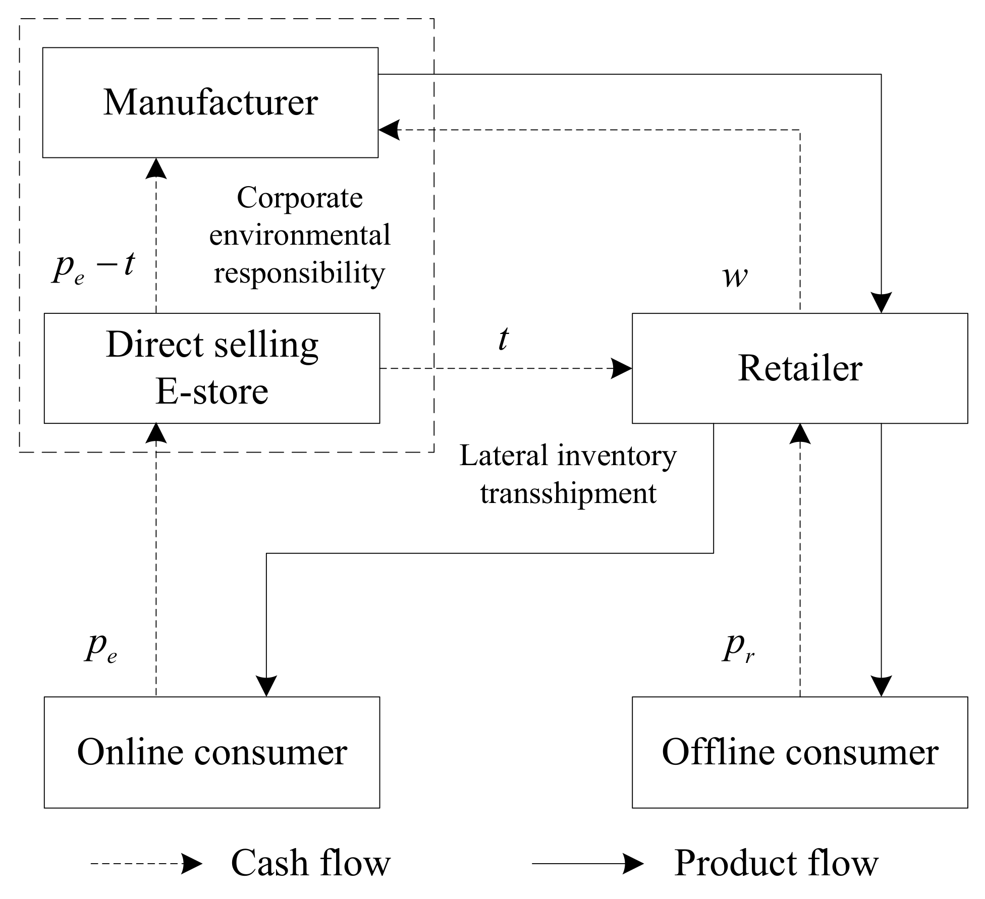
3.1. Problem Description
- (1)
- How to build demand functions and profit functions of online-to-offline supply chain firms considering manufacturer’s corporate environmental responsibility and lateral inventory transshipment.
- (2)
- How to construct the joint pricing and corporate environmental responsibility-level decision models for three decision scenarios.
- (3)
- How to coordinate online-to-offline supply chain in retailer and manufacturer Stackelberg games.
- (4)
- How do model parameters affect optimal policies of supply chain for three decision scenarios and coordination conditions in retailer and manufacturer Stackelberg games?
3.2. Notation and Basic Assumptions
4. Models and Equilibrium Results
4.1. Demand and Profit Functions
4.2. Scenario CD
- (1)
- Pricein the offline channel decreases with degreeif, but increases with degreeif.
- (2)
- Pricein the online channel decreases with degree.
- (3)
- Corporate environmental responsibility leveldecreases with degree.where.
- (1)
- Pricein the offline channel decreases with the online-to-offline service cost.
- (2)
- Pricein the online channel decreases with the online-to-offline service costif, but increases with the online-to-offline service costif.
- (3)
- Corporate environmental responsibility leveldecreases with the online-to-offline service cost.where.
4.3. Scenario RS
- (1)
- Margin pricein the offline channel decreases with degreeif, but increases with degreeif.
- (2)
- Wholesale pricein the offline channel decreases with degreeif, but increases with degreeif.
- (3)
- Retail pricein the offline channel decreases with degreeif, but increases with degreeif.
- (4)
- Retail pricein the online channel decreases with degree.
- (5)
- Corporate environmental responsibility leveldecreases with degree.where,
- (1)
- Margin pricein the offline channel increases with the online-to-offline service costif, but decreases with the online-to-offline service costif.
- (2)
- Wholesale pricein the offline channel decreases with the online-to-offline service costif, but increases with the online-to-offline service costif.
- (3)
- Retail pricein the offline channel decreases with the online-to-offline service costifor , but increases with the online-to-offline service costifor.
- (4)
- Retail pricein the online channel decreases with the online-to-offline service costif, but increases with the online-to-offline service costif.
- (5)
- Corporate environmental responsibility leveldecreases with the online-to-offline service costif, but increases with the online-to-offline service costif.where,.
- (1)
- Margin pricein the offline channel decreases with the online-to-offline service priceif, but increases with the online-to-offline service priceif.
- (2)
- Wholesale pricein the offline channel decreases with the online-to-offline service price.
- (3)
- Retail pricein the offline channel decreases with the online-to-offline service priceif, but increases with the online-to-offline service priceif.
- (4)
- Retail pricein the online channel decreases with the online-to-offline service priceif, but increases with the online-to-offline service priceif.
- (5)
- Corporate environmental responsibility leveldecreases with the online-to-offline service price.where,,.
4.4. Scenario MS
- (1)
- Margin pricein the offline channel decreases with degreeif, but increases with degreeif.
- (2)
- Wholesale pricein the offline channel decreases with degreeif, but increases with degreeif.
- (3)
- Retail pricein the offline channel decreases with degreeif, but increases with degreeif.
- (4)
- Retail pricein the online channel decreases with degree.
- (5)
- Corporate environmental responsibility leveldecreases with degree.where,,.
- (1)
- Margin pricein the offline channel decreases with the online-to-offline service cost.
- (2)
- Wholesale pricein the offline channel increases with the online-to-offline service cost.
- (3)
- Retail pricein the offline channel increases with the online-to-offline service costif, but decreases with the online-to-offline service costif.
- (4)
- Retail pricein the online channel increases with the online-to-offline service cost.
- (5)
- Corporate environmental responsibility levelincreases with the online-to-offline service cost.where.
- (1)
- Margin pricein the offline channel decreases with the online-to-offline service priceif, but increases with the online-to-offline service priceif.
- (2)
- Wholesale pricein the offline channel decreases with the online-to-offline service price.
- (3)
- Retail pricein the offline channel decreases with the online-to-offline service priceif, but increases with the online-to-offline service priceif.
- (4)
- Retail pricein the online channel decreases with the online-to-offline service priceif, but increases with the online-to-offline service priceif.
- (5)
- Corporate environmental responsibility leveldecreases with the online-to-offline service price.where ,,.
5. Coordination Analysis
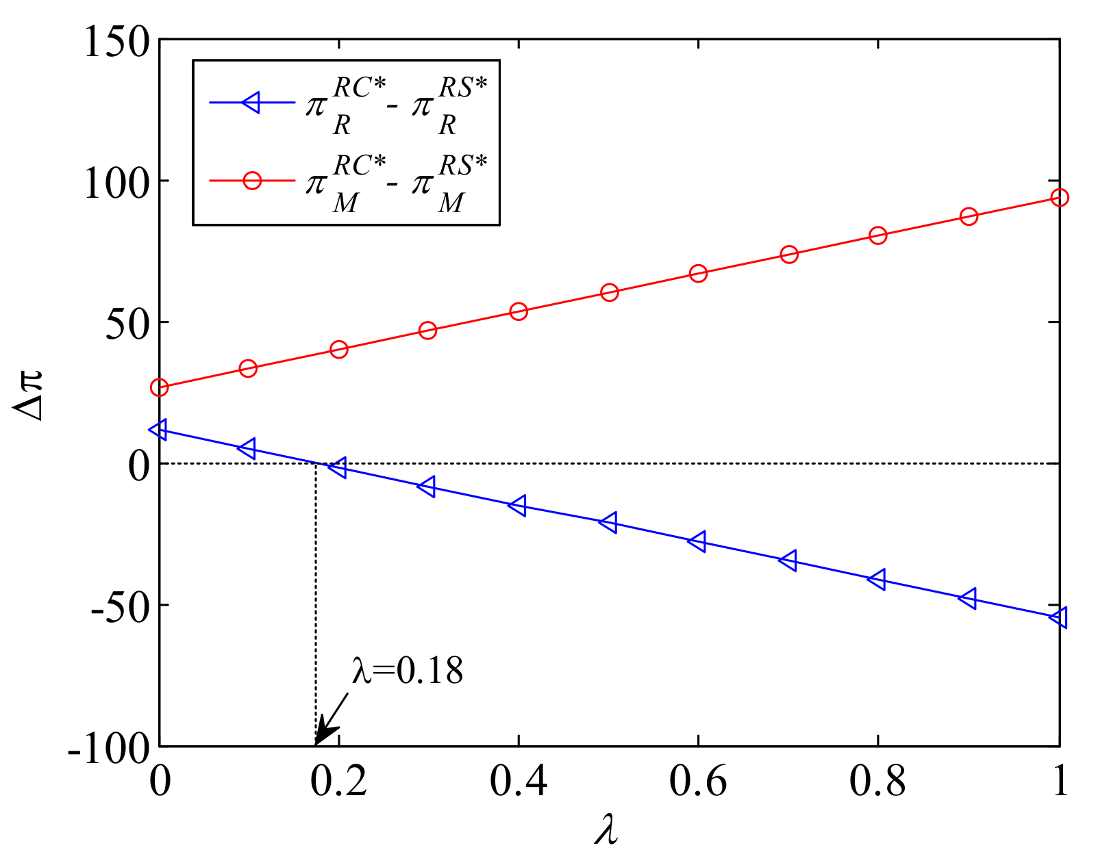
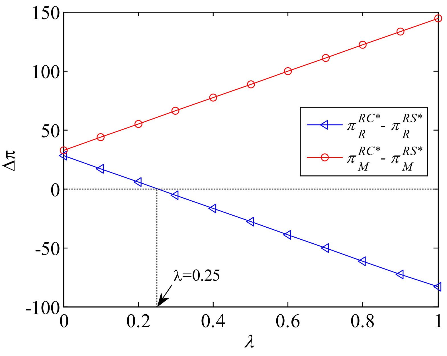
5.1. Scenario RS
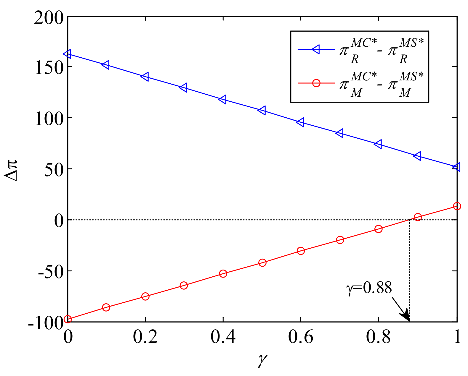
5.2. Scenario MS
6. Management Insights
7. Conclusions
Author Contributions
Funding
Institutional Review Board Statement
Informed Consent Statement
Data Availability Statement
Conflicts of Interest
Appendix A
References
- Kraus, S.; Rehman, S.; Sendra-Garcia, F. Corporate social responsibility and environmental performance: The mediating role of environmental strategy and green innovation. Technol. Forecast. Soc. 2020, 160, 120262. [Google Scholar] [CrossRef]
- Wu, H.; Li, G.; Xiao, S.; Li, H. Technology driven alliance for environmental and social responsibility in power supply chains. J. Clean. Prod. 2020, 276, 23194. [Google Scholar] [CrossRef]
- Wu, W.; Zhang, Q.; Liang, Z. Environmentally responsible closed-loop supply chain models for joint environmental responsibility investment, recycling and pricing decisions. J. Clean. Prod. 2020, 259, 120776. [Google Scholar] [CrossRef]
- Song, X.; Lu, Y.; Shen, L.; Shi, X. Will China′s building sector participate in emission trading system? Insights from modelling an owner’s optimal carbon reduction strategies. Energ. Policy 2018, 118, 232–244. [Google Scholar] [CrossRef]
- Song, X.; Shen, M.; Lu, Y.; Shen, L.; Zhang, H. How to effectively guide carbon reduction behavior of building owners under emission trading scheme? An evolutionary game-based study. Environ. Impact Asses. 2021, 90, 106624. [Google Scholar] [CrossRef]
- Stekelorum, R.; Laguir, I.; ElBaz, J. Can you hear the Eco? From SME environmental responsibility to social requirements in the supply chain. Technol. Forecast. Soc. 2020, 158, 120169. [Google Scholar] [CrossRef]
- Xia, J.; Niu, W. Carbon-reducing contract design for a supply chain with environmental responsibility under asymmetric information. Omega 2021, 102, 102390. [Google Scholar] [CrossRef]
- Li, Y.; Xiong, Y.; Mariuzzo, F.; Xia, S. The underexplored impacts of online consumer reviews: Pricing and new product design strategies in the O2O supply chain. Int. J. Prod. Econ. 2021, 237, 108148. [Google Scholar] [CrossRef]
- Pei, Z.; Wooldridge, B.; Swimberghe, K. Manufacturer rebate and channel coordination in O2O retailing. J. Retail. Consum. Serv. 2021, 58, 102268. [Google Scholar] [CrossRef]
- Yan, R.; Cao, Z. Product returns, asymmetric information, and firm performance. Int. J. Prod. Econ. 2017, 185, 211–222. [Google Scholar] [CrossRef]
- Yan, R.; Pei, Z.; Ghose, S. Reward points, profit sharing, and valuable coordination mechanism in the O2O era. Int. J. Prod. Econ. 2019, 215, 34–47. [Google Scholar] [CrossRef]
- Wu, Y.; Lu, R.; Yang, J.; Xu, F. Low-carbon decision-making model of online shopping supply chain considering the O2O model. J. Retail. Consum. Serv. 2021, 59, 102388. [Google Scholar] [CrossRef]
- Wu, Y.; Lu, R.; Yang, J.; Wang, R.; Xu, H.; Jiang, C. Government-led low carbon incentive model of the online shopping supply chain considering the O2O model. J. Clean. Prod. 2021, 279, 123271. [Google Scholar] [CrossRef]
- Zhao, F.; Wu, D.; Liang, L.; Dolgui, A. Lateral inventory transshipment problem in online-to-offline supply chain. Int. J. Prod. Res. 2016, 54, 1951–1963. [Google Scholar] [CrossRef]
- Nakandala, D.; Lau, H.; Zhang, J. Strategic hybrid lateral transshipment for cost-optimized inventory management. Ind. Manag. Data. Syst. 2016, 117, 1632–1649. [Google Scholar] [CrossRef]
- Nakandala, D.; Lau, H.; Shum, P. A lateral transshipment model for perishable inventory management. Int. J. Prod. Res. 2017, 55, 5341–5354. [Google Scholar] [CrossRef]
- Chen, X.; Wang, X.; Jiang, X. The impact of power structure on the retail service supply chain with an O2O mixed channel. J. Oper. Res. Soc. 2016, 67, 294–301. [Google Scholar] [CrossRef]
- Kong, L.; Liu, Z.; Pan, Y.; Xie, J.; Yang, G. Pricing and service decision of dual-channel operations in an O2O closed-loop supply chain. Ind. Manag. Data Syst. 2017, 117, 1567–1588. [Google Scholar] [CrossRef]
- He, P.; He, Y.; Xu, H.; Zhou, L. Online selling mode choice and pricing in an O2O tourism supply chain considering corporate social responsibility. Electron. Commer. Res. Appl. 2019, 38, 100894. [Google Scholar] [CrossRef]
- Sarkar, B.; Ullah, M.; Choi, S. Joint inventory and pricing policy for an online to offline closed-loop supply chain model with random defective rate and returnable transport items. Mathematics 2019, 7, 497. [Google Scholar] [CrossRef] [Green Version]
- Zheng, Y.; Liu, L.; Shi, V.; Liu, B.; Huang, W. Price cap models in pharmaceutical online-to-offline supply chains. Complexity 2020, 2020, 7471948. [Google Scholar] [CrossRef]
- Chai, L.; Duan, Y.; Huo, Z. Pricing strategies for O2O business model considering service spillover and power structures. Int. T. Oper. Res. 2021, 28, 1978–2001. [Google Scholar] [CrossRef]
- Yu, X.; Wang, S.; Zhang, X. Ordering decision and coordination of a dual-channel supply chain with fairness concerns under an online-to-offline model. Asia Pac. J. Oper. Res. 2019, 36, 1940004. [Google Scholar] [CrossRef]
- He, Y.; Zhang, J.; Gou, Q.; Bi, G. Supply chain decisions with reference quality effect under the O2O environment. Ann. Oper. Res. 2018, 268, 273–292. [Google Scholar] [CrossRef]
- Yan, Y.; Zhao, R.; Liu, Z. Strategic introduction of the marketplace channel under spillovers from online to offline sales. Eur. J. Oper. Res. 2018, 267, 65–77. [Google Scholar] [CrossRef]
- Zend, F.; Yaghoubi, S.; Sadjadi, S. Impacts of government direct limitation on pricing, greening activities and recycling management in an online to offline closed loop supply chain. J. Clean. Prod. 2019, 215, 1327–1340. [Google Scholar] [CrossRef]
- Ma, D.; Hu, J.; Wang, W. Differential game of product-service supply chain considering consumers’ reference effect and supply chain members’ reciprocity altruism in the online-to-offline mode. Ann. Oper. Res. 2021, 304, 263–297. [Google Scholar] [CrossRef]
- Ma, D.; Hu, J.; Yao, F. Big data empowering low-carbon smart tourism study on low-carbon tourism O2O supply chain considering consumer behaviors and corporate altruistic preferences. Comput. Ind. Eng. 2021, 153, 107061. [Google Scholar] [CrossRef]
- Sarkar, B.; Dey, B.; Sarkar, M.; AlArjani, A. A sustainable online-to-offline (O2O) retailing strategy for a supply chain management under controllable lead time and variable demand. Sustainability 2021, 13, 1756. [Google Scholar] [CrossRef]
- Sett, B.; Dey, B.; Sarkar, B. The effect of O2O retail service quality in supply chain management. Mathematics 2020, 8, 1743. [Google Scholar] [CrossRef]
- Xu, Q.; Fu, G.; Fan, D. Service sharing, profit mode and coordination mechanism in the Online-to-Offline retail market. Econ. Model. 2020, 91, 659–669. [Google Scholar] [CrossRef]
- Sun, C.; Ye, L.; Zhang, N. O2O selection mode portrait and optimization for railway service enterprises based on K-means. Complex Intell. Syst. 2021. Available online: https://doi.org/10.1007/s40747-021-00375-0 (accessed on 10 October 2021).
- Melacini, M.; Perotti, S.; Rasini, M.; Tappia, E. E-fulfilment and distribution in omni-channel retailing: A systematic literature review. Int. J. Phys. Distr. Log. 2018, 48, 391–414. [Google Scholar] [CrossRef]
- Cai, Y.; Lo, C. Omni-channel management in the new retailing era: A systematic review and future research agenda. Int. J. Prod. Econ. 2020, 229, 107729. [Google Scholar] [CrossRef]
- Jiang, Y.; Liu, L.; Lim, A. Optimal pricing decisions for an omni-channel supply chain with retail service. Int. T. Oper. Res. 2020, 27, 2927–2948. [Google Scholar] [CrossRef]
- Liu, L.; Feng, L.; Xu, B.; Deng, W. Operation strategies for an omni-channel supply chain: Who is better off taking on the online channel and offline service. Electron. Commer. Res. Appl. 2020, 39, 100918. [Google Scholar] [CrossRef]
- Wu, J.; Zhao, C.; Yan, X.; Wang, L. An integrated randomized pricing strategy for omni-channel retailing. Int. J. Electron. Comm. 2020, 24, 391–418. [Google Scholar] [CrossRef]
- Li, M.; Zhang, X.; Dan, B. Cooperative advertising and pricing in an O2O supply chain with buy-online-and-pick-up-in-store. Int. T. Oper. Res. 2021, 28, 2033–2054. [Google Scholar] [CrossRef]
- Chen, Z.; Su, S. Consignment supply chain cooperation for complementary products under online to offline business mode. Flex. Serv. Manuf. J. 2021, 33, 136–182. [Google Scholar] [CrossRef]
- Karray, S.; Sigue, S. Offline retailers expanding online to compete with manufacturers: Strategies and channel power. Ind. Market. Manag. 2018, 71, 203–214. [Google Scholar] [CrossRef]
- Sarkar, B.; Tayyab, M.; Choi, S. Product channeling in an O2O supply chain management as power transmission in electric power distribution systems. Mathematics 2019, 7, 4. [Google Scholar] [CrossRef] [Green Version]
- Wen, D.; Xiao, T.; Dastani, M. Pricing and collection rate decisions in a closed-loop supply chain considering consumers′ environmental responsibility. J. Clean. Prod. 2020, 262, 121272. [Google Scholar] [CrossRef]
- Yuan, X.; Tang, F.; Zhang, D.; Zhang, X. Green remanufacturer’s mixed collection channel strategy considering enterprise′s environmental responsibility and the fairness concern in reverse green supply chain. Int. J. Env. Res. Pub. He. 2021, 18, 3405. [Google Scholar] [CrossRef] [PubMed]
- Hong, Z.; Guo, X. Green product supply chain contracts considering environmental responsibilities. Omega 2019, 83, 155–166. [Google Scholar] [CrossRef]
- Heydari, J.; Rafiei, P. Integration of environmental and social responsibilities in managing supply chains: A mathematical modeling approach. Comput. Ind. Eng. 2020, 145, 106495. [Google Scholar] [CrossRef]
- Xie, L.; Ma, J.; Goh, M. Supply chain coordination in the presence of uncertain yield and demand. Int. J. Prod. Res. 2021, 59, 4342–4358. [Google Scholar] [CrossRef]
- Heydari, J.; Govindan, K.; Basiri, Z. Balancing price and green quality in presence of consumer environmental awareness: A green supply chain coordination approach. Int. J. Prod. Res. 2021, 59, 1957–1975. [Google Scholar] [CrossRef]
- Lee, J.; Kim, Y.; Kim, Y. Antecedents of adopting corporate environmental responsibility and green practices. J. Bus. Ethics. 2018, 148, 397–409. [Google Scholar] [CrossRef]
- Yang, D.; Xiao, T.; Huang, J. Dual-channel structure choice of an environmental responsibility supply chain with green investment. J. Clean. Prod. 2019, 210, 134–145. [Google Scholar] [CrossRef]
- Wu, Y.; Wang, J.; Li, C.; Su, K. Optimal supply chain structural choice under horizontal chain-to-chain competition. Sustainability 2018, 10, 1330. [Google Scholar] [CrossRef] [Green Version]
- Carbone, V.; Moatti, V.; Schoenherr, T.; Gavirneni, S. From green to good supply chains: Halo effect between environmental and social responsibility. Int. J. Phys. Distr. Log. 2019, 49, 839–860. [Google Scholar] [CrossRef]
- Qin, Y.; Harrison, J.; Chen, L. A framework for the practice of corporate environmental responsibility in China. J. Clean. Prod. 2019, 235, 426–452. [Google Scholar] [CrossRef]
- Plambeck, E.; Taylor, T. Supplier evasion of a buyer′s audit: Implications for motivating supplier social and environmental responsibility. M&SOM Manuf. Serv. Op. 2016, 18, 184–197. [Google Scholar]
- Dey, P.; Petridis, N.; Petridis, K.; Malesios, C.; Nixon, J.; Ghosh, S. Environmental management and corporate social responsibility practices of small and medium-sized enterprises. J. Clean. Prod. 2018, 195, 687–702. [Google Scholar] [CrossRef] [Green Version]
- Kogg, B.; Mont, O. Environmental and social responsibility in supply chains: The practise of choice and inter-organisational management. Ecol. Econ. 2012, 83, 154–163. [Google Scholar] [CrossRef]
- Kovacs, C. Corporate environmental responsibility in the supply chain. J. Clean. Prod. 2008, 16, 1571–1578. [Google Scholar] [CrossRef]
- Villena, V.; Wilhelm, M.; Xiao, C. Untangling drivers for supplier environmental and social responsibility: An investigation in Philips Lighting′s Chinese supply chain. J. Oper. Manag. 2021, 67, 476–510. [Google Scholar] [CrossRef]
- Tuczek, F.; Castka, P.; Wakolbinger, T. A review of management theories in the context of quality, environmental and social responsibility voluntary standards. J. Clean. Prod. 2018, 176, 399–416. [Google Scholar] [CrossRef]
- Herer, Y.; Rashit, A. Lateral stock transshipments in a two-location inventory system with fixed and joint replenishment costs. Nav. Res. Log. 1999, 46, 525–547. [Google Scholar] [CrossRef]
- Firouz, M.; Keskin, B.; Melouk, S. An integrated supplier selection and inventory problem with multi-sourcing and lateral transshipments. Omega 2016, 70, 77–93. [Google Scholar] [CrossRef]
- Meissner, J.; Senicheva, O. Approximate dynamic programming for lateral transshipment problems in multi-location inventory systems. Eur. J. Oper. Res. 2017, 265, 49–64. [Google Scholar] [CrossRef]
- Grahovac, J.; Chakravarty, A. Sharing and lateral transshipment of inventory in a supply chain with expensive low-demand items. Manag. Sci. 2001, 47, 579–594. [Google Scholar] [CrossRef]
- Shokouhifar, M.; Sabbaghi, M.; Pilevari, N. Inventory management in blood supply chain considering fuzzy supply/demand uncertainties and lateral transshipment. Transfus. Apher. Sci. 2021, 60, 103103. [Google Scholar] [CrossRef] [PubMed]
- Naseraldin, H.; Herer, Y. A location-inventory model with lateral transshipments. Nav. Res. Log. 2011, 58, 437–456. [Google Scholar] [CrossRef]
- Yang, G.; Dekker, R.; Gabor, F.; Axsater, S. Service parts inventory control with lateral transshipment and pipeline stock flexibility. Int. J. Prod. Res. 2012, 142, 278–289. [Google Scholar] [CrossRef]
- Paterson, C.; Kiesmuller, G.; Teunter, R.; Glazebrook, K. Inventory models with lateral transshipments: A review. Eur. J. Oper. Res. 2011, 210, 125–136. [Google Scholar] [CrossRef] [Green Version]
- Gilbert, S.; Cvsa, V. Strategic commitment to price to stimulate downstream innovation in a supply chain. Eur. J. Oper. Res. 2003, 150, 617–639. [Google Scholar] [CrossRef]
- Savaskan, R.; Bhattacharya, S.; Van-Wassenhove, L. Closed-loop supply chain models with product remanufacturing. Manag. Sci. 2004, 50, 239–252. [Google Scholar] [CrossRef] [Green Version]
- Li, T.; Tan, Q.; Liu, W. Game theoretical perspectives on pricing decisions in asymmetric competing supply chains. Discret. Dyn. Nat. Soc. 2020, 2020, 9352013. [Google Scholar] [CrossRef]
- Cao, B.; Gong, Z.; You, T. Stackelberg pricing policy in dyadic capital-constrained supply chain considering bank′s deposit and loan based on delay payment scheme. J. Ind. Manag. Optim. 2021, 17, 2855–2887. [Google Scholar]
- Huang, S.; Fan, Z.P.; Wang, N. Green subsidy modes and pricing strategy in a capital-constrained supply chain. Transp. Res. Part E Logisy. Transp. Rev. 2020, 136, 101885. [Google Scholar] [CrossRef]
- Taleizadeh, A.; Sanezerang, E.; Choi, T. The effect of marketing effort on dual-channel closed-loop supply chain systems. IEEE Trans. Syst. Man Cybern. Syst. 2018, 48, 265–276. [Google Scholar] [CrossRef]
- Taleizadeh, A.; Hazarkhani, B.; Moon, L. Joint pricing and inventory decisions with carbon emission considerations, partial backordering and planned discounts. Ann. Oper. Res. 2020, 290, 95–113. [Google Scholar] [CrossRef]
- Tsendsuren, C.; Yadav, R.; Han, S.; Kim, H. Influence of product market competition and managerial competency on corporate environmental responsibility: Evidence from the US. J. Clean. Prod. 2021, 304, 127065. [Google Scholar] [CrossRef]
- Taleizadeh, A.; Cheraghi, Z.; Cardenas-Barron, L.; Noori-Daryan, M. Studying the effect of noise on pricing and marketing decisions of new products under co-op advertising strategy in supply chains: Game theoretical approaches. Mathematics 2021, 9, 1222. [Google Scholar] [CrossRef]
- Cao, B.; Fan, Z.; You, T. The optimal pricing and ordering policy for temperature sensitive products considering the effects of temperature on demand. J. Ind. Manag. Optim. 2019, 15, 1153–1184. [Google Scholar] [CrossRef]
- Zhu, Q.; Li, X.; Zhao, S. Cost-sharing models for green product production and marketing in a food supply chain. Ind. Manag. Data Syst. 2018, 118, 654–682. [Google Scholar] [CrossRef]
- Phan, D.; Vo, T.; Lai, A.; Nguyen, T. Coordinating contracts for VMI systems under manufacturer-CSR and retailer-marketing efforts. Int. J. Prod. Econ. 2019, 211, 98–118. [Google Scholar] [CrossRef]
- Cao, B.; Fan, Z. Ordering and sales effort investment for temperature sensitive products considering retailer′s disappointment aversion and elation seeking. Int. J. Prod. Res. 2018, 56, 2411–2436. [Google Scholar] [CrossRef]
- Liu, Y.; Li, J.; Quan, B.; Yang, J. Decision analysis and coordination of two-stage supply chain considering cost information asymmetry of corporate social responsibility. J. Clean. Prod. 2019, 228, 1073–1087. [Google Scholar] [CrossRef]
- Lou, G.; Lai, Z.; Ma, H.; Fan, T. Coordination in a composite green-product supply chain under different power structures. Ind. Manag. Data Syst. 2020, 120, 1101–1123. [Google Scholar] [CrossRef]
- Shang, W.; Yang, L. Contract negotiation and risk preferences in dual-channel supply chain coordination. Int. J. Prod. Res. 2015, 53, 4837–4856. [Google Scholar] [CrossRef]


| References | Online-to-Offline Supply Chain | Pricing | Coordination | Corporate Environmental Responsibility | Lateral Inventory Transshipment |
|---|---|---|---|---|---|
| Zhao et al. [14] | √ | √ | |||
| Sarkar et al. [20] | √ | √ | |||
| Chai et al. [22] | √ | √ | |||
| Yu et al. [23] | √ | √ | √ | ||
| Jiang et al. [35] | √ | √ | |||
| Wen et al. [42] | √ | √ | |||
| Yuan et al. [43] | √ | √ | |||
| Yang et al. [49] | √ | √ | |||
| Shokouhifar et al. [63] | √ | ||||
| Our study | √ | √ | √ | √ | √ |
| Decision variables: | |
| : | The wholesale price of manufacturer in the offline channel, . |
| : | The margin price of retailer in the offline channel, . |
| : | The retail price of retailer in the offline channel, . It is necessary to point out that, in Scenarios RS and MS, will be not decision variable since . |
| : | The retail price of manufacturer in online channel, . |
| : | The corporate environmental responsibility level of manufacturer, . |
| Parameters: | |
| : | The market size, . |
| : | The preference degree of the consumer to the offline channel in purchasing decision, . |
| : | The self-price elasticity, it is used to describe the impact of unit change of retail price on demand in current channel, . |
| : | The cross-price elasticity, it is used to describe the impact of unit change of retail price in a competitive channel on demand in current channel, . |
| : | The online-to-offline service price of retailer, it is paid by the manufacturer to the retailer for unit product in online-to-offline mode with lateral inventory transshipment, . |
| : | The online-to-offline service cost of retailer. The retailer needs to bear it for unit product in an online-to-offline mode with lateral inventory transshipment, . |
| : | The unit production cost of manufacturer, . |
| : | The corporate environmental responsibility sensitivity, it is used to describe the impact of unit change of corporate environmental responsibility level on market demand in the offline or online channel, where denotes offline or online channel, respectively, . |
| : | The investment cost sensitivity to corporate environmental responsibility, it is used to describe the impact of unit corporate environmental responsibility level on the profit of manufacturer, . |
| : | The revenue sharing rate for Scenario RS in coordination analysis, . |
| : | The revenue sharing rate for Scenario MS in coordination analysis, . |
| Functions: | |
| : | The demand function of offline or online channel, . |
| : | The profit function of retailer, manufacturer, or supply chain, . |
| ↓↑ | ↓ | - | |
| ↓ | ↓↑ | - | |
| ↓ | ↓ | - |
| ↓↑ | ↑↓ | ↓↑ | |
| ↓↑ | ↓↑ | ↓ | |
| ↓↑ | ↓↑↓ | ↓↑ | |
| ↓ | ↓↑ | ↓↑ | |
| ↓ | ↓↑ | ↓ |
| ↓↑ | ↓ | ↓↑ | |
| ↓↑ | ↑ | ↓ | |
| ↓↑ | ↑↓ | ↓↑ | |
| ↓ | ↑ | ↓↑ | |
| ↓ | ↑ | ↓ |
Publisher’s Note: MDPI stays neutral with regard to jurisdictional claims in published maps and institutional affiliations. |
© 2021 by the authors. Licensee MDPI, Basel, Switzerland. This article is an open access article distributed under the terms and conditions of the Creative Commons Attribution (CC BY) license (https://creativecommons.org/licenses/by/4.0/).
Share and Cite
Cao, B.; You, T.; Liu, C.; Zhao, J. Pricing and Channel Coordination in Online-to-Offline Supply Chain Considering Corporate Environmental Responsibility and Lateral Inventory Transshipment. Mathematics 2021, 9, 2623. https://doi.org/10.3390/math9202623
Cao B, You T, Liu C, Zhao J. Pricing and Channel Coordination in Online-to-Offline Supply Chain Considering Corporate Environmental Responsibility and Lateral Inventory Transshipment. Mathematics. 2021; 9(20):2623. https://doi.org/10.3390/math9202623
Chicago/Turabian StyleCao, Bingbing, Tianhui You, Chunyi Liu, and Jian Zhao. 2021. "Pricing and Channel Coordination in Online-to-Offline Supply Chain Considering Corporate Environmental Responsibility and Lateral Inventory Transshipment" Mathematics 9, no. 20: 2623. https://doi.org/10.3390/math9202623
APA StyleCao, B., You, T., Liu, C., & Zhao, J. (2021). Pricing and Channel Coordination in Online-to-Offline Supply Chain Considering Corporate Environmental Responsibility and Lateral Inventory Transshipment. Mathematics, 9(20), 2623. https://doi.org/10.3390/math9202623