Improved Multi-Scale Deep Integration Paradigm for Point and Interval Carbon Trading Price Forecasting

Abstract

The forecast of carbon trading price is crucial to both sellers and purchasers; multi-scale integration models have been used widely in this process. However, these multi-scale models ignore the feature reconstruction process as well as the residual part and also they often focus on the linear integration. Meanwhile, most of the models cannot provide prediction interval which means they neglect the uncertainty. In this paper, an improved multi-scale nonlinear integration model is proposed. The original dataset is divided into some subgroups through variational mode decomposition (VMD) and all the subgroups will go through sample entropy (SE) process to reconstruct the features. Then, random forest and long-short term memory (LSTM) integration are used to model feature sub-sequences. For the residual part, LSTM residual correction strategy based on white noise test corrects residuals to obtain point prediction results. Finally, Gaussian process (GP) is applied to get the prediction interval estimate. The result shows that compared with some other methods, the proposed method can obtain satisfying accuracy which has the minimum statistical error. So, it is safe to conclude that the proposed method is able to efficiently predict the carbon price as well as to provide the prediction interval estimate.

1. Introduction

The global warming has posed a challenge to the world, and many countries as well as regions have begun to adopt the carbon emission trading approaches to effectively control greenhouse gas emissions [1] in an effort to reach the 26–28% target required by the 2030 Paris Agreement [2]. Meanwhile, China, known as the world second largest economy and the largest developing country, has become the biggest carbon emitter in the world, to cope with this situation, China has proposed a 60–65% reduction target in CO₂ emissions from 2005 levels by 2030 [3]. China established a national emission trading system (ETS) to peak its carbon emission around 2030, building on the experience of pilot ETSs that are planned to be linked [4]. China has also implemented a tradable green certificate market on the basis of the carbon emissions trading market [5]. Based on this, carbon trading market in China has been developing during recent years where carbon trading is the main process. The fundamental purpose of building a carbon emission trading market is to correct market failures and better play the decisive role of the market in the allocation of climate capacity resources. Through the development of the carbon market, our country has formed a carbon price mechanism covering key industries, and has transmitted it through the market to provide the market with long-term stable carbon price expectations, thereby influencing the investment and consumer behavior decisions of stakeholders, and promoting the transformation of country’s green and low-carbon development.

In the initial stage, the government will allocate carbon emission credits to participating companies for free, which means that companies will only need to pay additional costs after they have exhausted their quotas. The carbon trading market forces companies to purchase emission permits from companies that have surplus allowances after exhausting their emission allowances.

That said, carbon trading has not only become a key point in reducing greenhouse gas emissions but also a significant tool to investment. To obtain full profit for sellers and to reach the most reasonable purchasing price for buyers, the prediction of the carbon price has been attracting much attention to generate the most accurate result.

During recent years, multi-scale integration models have been used widely in this field and scholars have proposed various approaches for carbon price forecasting, many of them have achieved satisfying accuracy while some need to be improved. These models can be generally classified into two parts: the decomposition part and the prediction part.

For the decomposition part, the methods mainly include wavelet transform (WT) [6], empirical mode decomposition (EMD) [7,8], and variational mode decomposition (VMD) [9]. The basic method is WT which is mainly applicable when the frequency bands of useful signal and noise are separated from each other [10] and in these cases, WT shows great performance. However, WT has limitations of poor adaptation and the number of layers needs to be set, making WT difficult to apply in the price series decomposition. In this case, EMD and its variants such as ensemble empirical mode decomposition (EEMD) [11], fast ensemble empirical model decomposition (FEEMD) [12], and mean value optimization empirical model decomposition (MOEMD) [13] are proposed to improve the capability which do better in adaption. Similarly, EMD has problem of performing weak for lack of physical meaning. To make up for this, VMD rises which is superior to EMD-based noise reduction and discrete wavelet threshold filtering [14]. Still, VMD is adaptable no matter it is in secondary decomposition [15] or serves as the basis of the combination of other methods [16].

Usually when decomposition is finished, it comes to the part of prediction. For the prediction part, the methods can be further classified into two categories as well: the classic statistical methods and the machine learning methods. To start with, the classic statistical method is still of usage. They are easy to operate and the predicting accuracy in many cases is satisfying. The mostly used methods are the autoregressive integrated moving average model (ARIMA) [17,18] and generalized autoregressive conditional heteroskedasticity model (GARCH) [19,20,21,22]. However, the statistical methods have some obvious shortcomings [23] in that they usually have strict normality assumptions which is often not the case in the price series, and they are often used for linear processing while price series contains many nonlinear features.

To extract nonlinear features, machine learning (including deep learning) methods have become hot spots. Of all the methods, artificial neural network (ANN), support vector machine (SVM), random forest, and long-short term memory (LSTM) are the mostly used methods. ANN has strong parallel distribution processing ability, strong robustness, and fault tolerance to noise nerves [24], making it a hot tool in the price series processing task [25]. Prediction models established based on ANN usually have higher accuracy and faster convergence speed [26,27,28]. However, the drawback of ANN is that sometimes the learning time is too long, and may not even achieve the purpose of learning. Under this situation, SVM is proposed. SVM (as well as its variants such as least square support vector machine (LSSVM) [29,30]) can solve machine learning problems in the case of small samples and can improve generalization performance which is proved to be an advanced method for predicting high non-stationary and non-linearity series [31,32,33]. But the weakness of SVM cannot be ignored, it does not have a strong solution to multi-classification problems. Moreover, SVM is very sensitive to the selection of parameters and kernel functions making them unstable in the predicting period.

Not only in order to efficiently handle large-scale samples or high-dimensional data, but also to balance errors, random forest is developed. Random forest has strong generalization ability and can also process data of very high dimensions without making feature selection [34]. When it is trained fully, random forest can decide which features are more important [35]. It can also be utilized to calculate the energy carbon footprint as well as to verify the performance of the random forest algorithm [36] and it is proved to be able to improve the accuracy of prediction compared with ANN [37]. As for LSTM, a useful tool of deep learning, it stands out with better performance. LSTM can effectively retain historical information and realize the learning of the long-term dependent information [38,39,40], making it suitable for time series forecasting [41]. When compared with other popular methods such as backpropagation, SVM, LSTM provides better performance and predicting accuracy [42], therefore, LSTM has been applied more and more in the price series prediction [43]. These reasons are also why this paper chooses the random forest and LSTM as parts.

Although these multi-scale integration methods have shown some great advantages, many of them also have shortcomings. To start with, the sub-sequences will usually go through the following process without feature reconstruction, which means even some sub-sequences are not suitable, they will still be part of the prediction process and this will have a negative effect on the final prediction result. Then, many studies will simply apply linear accumulation for integration which means the integration job is carried out by simple adding, doing this clearly ignores the nonlinear features in the time series. Meanwhile, in many research, the prediction process ignores the residual part but as a matter of fact, there will be some useful information left in the residual series, if neglected, the whole process will have the problem of information loss. Finally, the existing research will merely be satisfied with the point prediction without the concern about interval prediction. Due to this, the prediction will show low fault tolerance.

It is known to all that as a kind of time series, the carbon trading price has the characteristics of variability, difficulty in grasping and sensitivity, and so on, making the precise prediction of it a tough task; and this can explain why many of the existing work cannot actually handle this mission to the largest degree. In this paper, as well as aiming at the reasons above, an improved multi-scale nonlinear ensemble model coupled Gaussian process (GP) is proposed, which follows the efficient framework: the decomposition and prediction framework. In the decomposition part, VMD will be combined with SE to serve as the feature reconstruction process to guarantee the sub-sequences will be the most suitable. Then, for the prediction part, first, random forest is the tool of sub-sequence prediction. Afterwards, the sub-results will be integrated by LSTM to form the first result. Then, white noise test is carried out to see whether the residual series is a white noise series, if it is, the residual will go through LSTM again and then be added back to the first result. What needs to be emphasized is that when the point prediction is obtained, GP is applied to generate the prediction interval estimate.

The innovation can be concluded as follows:

(A)

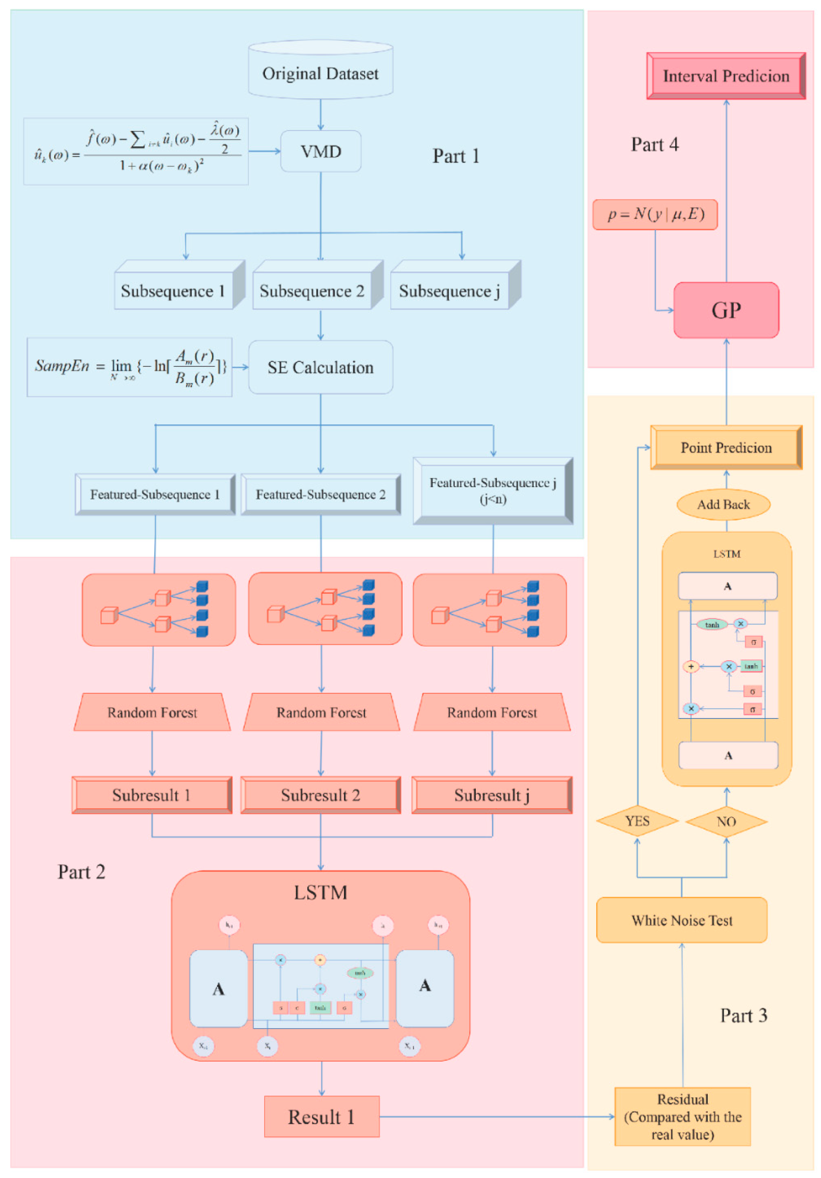
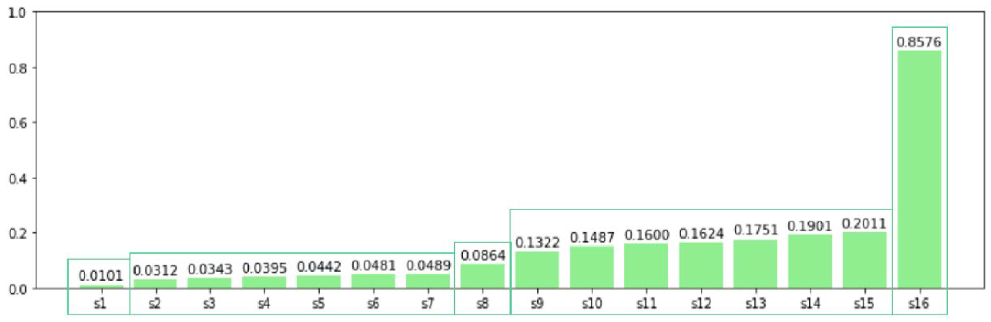
Instead of carrying out research on the original data series, this paper decomposes the series first, in this way, the features of the series are separated, making the process that follows more targeted. Moreover, some sub-sequences can include similar features, there is no need to divide them too much, so the feature reconstruction process will also be included. In the proposed model, VMD combined with SE not only decomposes the series but also reconstructs the features. These methods can be seen as a system which performs the feature extraction and noise elimination work;

(B)

The proposed model applies the two-step learning process which includes random forest and LSTM rather than simple one-step learning or simple linear accumulation for they will usually leave the problem of messy learning or incomplete learning. The two-step nonlinear learning will make the learning process more targeted and also more complete;

(C)

The residual will also be seen as an important part of the whole process which goes through the LSTM to do the correction work. This means the residual will be added back after LSTM process to the first prediction result and in this way, the final prediction result will be obtained. Paying attention to the residual series will capture the useful information left, which shows the effort to grasp the important features as much as possible;

(D)

Many existing work will be satisfied merely with the point prediction result but this brings high uncertainty and low fault tolerance. As a result, this paper reflects the idea of interval estimate, which shows great improvement in the fault tolerance.

The rest of the paper is organized as follows: the second section is the related methodology introduction. The third part displays the flowchart of the proposed model. The fourth section carries out the case study of the proposed model. In the fifth section, different models are compared and discussed. The sixth part gives the conclusion.

2. Related Methodology

This study proposes an improved multi-scale nonlinear integration model. In this section, the following main methods applied by the proposed model will be introduced: variational mode decomposition (VMD), random forest, long-short term memory (LSTM), and Gaussian process (GP). The remaining assistant methods will be introduced in the Appendix A namely sample entropy (SE) and white noise test.

2.1. Variational Mode Decomposition

The main idea of VMD is that a signal is made up of sub-signals dominated by different frequencies. The aim is to decompose the signal into sub-signals of different frequencies. In this section, the main steps are shown.

Assuming the shorthand notations for the set of $K$ modes and their center frequencies are $\left\{{\mu }_k\right\}=\{{\mu }_1,{\mu }_2,\dots ,{\mu }_k\}$ and $\left\{{\omega }_k\right\}=\{{\omega }_1,{\omega }_2,\dots ,{\omega }_k\}$ separately, then, make $\delta$ as the Dirac distribution, $t$ as the time script, $j$ the imaginary number (which means $j^2=-1$), and * the convolution operator. Each mode ${\mu }_k$ needs to be mostly compact around the center pulsation ${\omega }_k$ which will be decided together with the decomposition. Meanwhile, in VMD, the sum of bandwidth of every mode is required (estimated by the $H^1$ Gaussian smoothness of the demodulated signal and this means the squared $L^2-norm$ is the least) to be equal to the original signal under the constraint condition. As a result, take a given time series $f$ as an example, the decomposition approach is equal to solving the following:

$$\underset{\left\{{\mu }_k\right\},\left\{{\omega }_k\right\}}{\min }{{\displaystyle \sum _k‖{\partial }_t[(\delta (t)+\frac{j}{\pi t})\ast {\mu }_k(t)]e^{-j{\omega }_{k}t}‖}}_2^2$$

(1)

To render the question, there needs to apply a quadratic penalty term and the Lagrangian multipliers $\lambda$. Therefore, the augmented Lagrangian will be:

$$\begin{array}{l}\mathcal{\ell }(\{{\mu }_k\},\{{\omega }_k\},\lambda )=\alpha {{\displaystyle \sum _k‖{\partial }_t[(\delta (t)+\frac{j}{\pi t})\ast {\mu }_k(t)]e-j{\omega }_{k}t‖}}_2^2\\ \hspace{1em}\hspace{1em}\hspace{1em}\hspace{1em}\hspace{1em}\hspace{1em}\hspace{0.17em}\hspace{0.17em}+{‖f(t)-{\displaystyle \sum _k{\mu }_k(t)}‖}_2^2+〈\lambda (t),f(t)-{\displaystyle \sum _k{\mu }_k(t)}〉\end{array}$$

(2)

here $\alpha$ is the balancing parameter; then the formula can be solved by the alternate direction method of multipliers. The mode is updated through the following:

$${\widehat{\mu }}_k^{n+1}(\omega )=\frac{\widehat{f}(\omega )-{\displaystyle {\sum }_{i\ne k}{\widehat{\mu }}_i(\omega )+\frac{\widehat{\lambda }(\omega )}{2}}}{1+2\alpha {(\omega -{\omega }_k)}^{{}_2}}$$

(3)

here ${\omega }_k$ is the center frequencies whose update formula is:

$${\widehat{\omega }}_k^{n+1}=\frac{{\displaystyle {\int }_0^{\infty }\omega {\left|{\widehat{\mu }}_k(\omega )\right|}^{2}d\omega }}{{\displaystyle {\int }_0^{\infty }{\left|{\widehat{\mu }}_k(\omega )\right|}^{2}d\omega }}$$

(4)

Meanwhile, the update formula of $\lambda$ is:

$${\widehat{\lambda }}^{n+1}(\omega )={\widehat{\lambda }}^n(\omega )+\tau (\widehat{f}(\omega )-{\displaystyle \sum _k{\widehat{\mu }}_k^{n+1}(\omega )})$$

(5)

The mode in time domain will be obtained through the real part of the inverse Fourier transform.

2.2. Random Forest

Random forest is an algorithm that uses multiple decision trees to train, classify, and predict samples, and is mainly used in regression and classification scenarios. The random forest contains many trees and each tree gives the classification result. The general rules of each tree are as follows:

(1)

If the size of the training set is $N$, for each tree, $N$ training samples are taken from the training randomly and with replacement. As the training set of the tree, it is repeated K times to generate $K$ sets of training sample sets.

(2)

If the sample dimension of each feature is $M$, specify a constant $m$ which is smaller than $M$, and randomly select $m$ features from the $M$ features.

(3)

Use $m$ features to maximize the growth of each tree with no pruning process.

During the process of model establishment, we first set up a set of unrelated regression decision trees $\{h(x,{\theta }_k),k=1,2,\dots ,K\}$ which contains $K$ individuals:

$$h(x)=\frac{1}{N}{\displaystyle \sum _{k=1}^{K}h(x,{\theta }_k)}$$

(6)

here ${\theta }_k$ means the independent and identically distributed random variables.

Then, according to rule (1), carry out random sampling with replacement, repeat sampling from the original sample data set to obtain K training samples equal to the original sample data set, and each training sample constitutes a decision tree. Afterwards, when regression trees are got, each split node randomly selects the features in all variables as the feature subset of the current node split, and selects the optimal splitting method for splitting in the feature subset. In random forest regression, the number of trees K and randomly selected node splitting characteristics determine the predictive ability of the model.

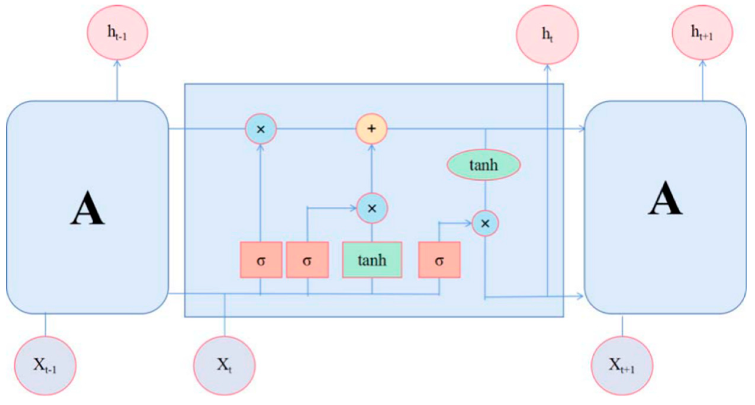
2.3. Long-Short Term Memory

LSTM is a type of recurrent neural network. The traditional recurrent neural network has such a problem of long-term dependence. When the distance between the prediction point and the dependent related information is relatively far, it is difficult to learn the related information. In theory, recurrent neural networks can handle such problems, but in reality, conventional recurrent neural networks cannot solve long-term dependencies well. Fortunately, LSTM can solve this problem. The general framework of LSTM is shown in Figure 1 [44]. The main steps can be summed up as follows [44]:

Step 1: Decide what information can pass the cell state. This decision is made by the forget gate layer using sigmoid, which will pass or partially pass according to the output of the previous moment.

Step 2: Generate new information needed to update. This step consists of two parts. To start with, an input gate layer that uses sigmoid determines which values are used for updating. Then, the second part, a tanh layer is used to generate new candidate values and add them.

Step 3: Determine the final output. When an initial output through the sigmoid layer is obtained, tanh is applied to make the values scaled from −1 to 1, then they are multiplied by the output obtained by sigmoid pair by pair to obtain the model output.

In the figure, $x_t$ is the input at time $t$; $h_t$ is the output at time $t$; $\sigma$ is the sigmoid function.

When applying LSTM in the time series prediction process, some important formulas are as follows [44]:

(1)

First, assume ${\tilde{c}}_t$ as the value of the candidate memory cell at time $t$; $w_c,b_c$ are the corresponding weight matrix and the corresponding bias to the cell, then there is:

$${\tilde{c}}_t=\tanh (w_c[h_{t-1},x_t]+b_c)$$

(7)

(2)

Calculate the value of input gate $i_t$:

$$i_t=\sigma (w_i[h_{t-1},x_t]+b_i)$$

(8)

(3)

Calculate the value of forget gate $f_t$:

$$f_t=\sigma (w_f[h_{t-1},x_t]+b_f)$$

(9)

(4)

Calculate the value of the current memory cell $c_t$:

$$c_t=f_t{c}_{t-1}+i_t{\tilde{c}}_t$$

(10)

(5)

Calculate the value of output gate $o_t$:

$$o_t=\sigma (w_o[h_{t-1},x_t]+b_o)$$

(11)

(6)

Then the general output of LSTM can be calculated:

$$h_t=o_t\tanh (c_t)$$

(12)

2.4. Gaussian Process

Gaussian process is carried out to form the prediction interval estimate. Then the main composition is discussed in this section.

The Gaussian process can usually be used to represent a function, more specifically, and the distribution of a function. Usually, for a function to be learned, first it needs to define the parameters of the function, and then learn the parameters of this function according to the training data. This method is called a parameterized method. But this approach limits the range of functions that can be learned, and it is impossible to learn any type of function. Non-parametric methods do not have this disadvantage. Using Gaussian processes to model functions is a nonparametric method.

Assuming there are two points: $x_0$ = 0 and $x_1$ = 1, the function values corresponding to these two points follow a two-dimensional Gaussian distribution:

$$\left(\begin{array}{l}{y}_0\\ y_1\end{array}\right)~N\left(\left(\begin{array}{l}0\\ 0\end{array}\right),\left(\begin{array}{l}1\hspace{1em}0\\ 0\hspace{1em}1\end{array}\right)\right)$$

(13)

where $y_0$ and $y_1$ are the function values corresponding to these two points.

If there are 20 $x$ points, the function values corresponding to these 20 points have a mean of 0, and the covariance matrix is the joint Gaussian distribution of the identity matrix. However, such a function is not smooth at all, and it looks messy. The function values corresponding to two points that are very close can be very different. Intuitively, the closer the two points are to each other, the smaller the corresponding function value should be, that is to say this function should be smooth, not abrupt. So, the covariance between the function values corresponding to these two points should be defined by some distance between the two points. As is mentioned above, the closer the two points are to each other, the larger the covariance between the corresponding function values should be, which means the closer the two function values may be.

Then, introduce Gaussian kernel function as:

$$k(x,x^{\prime })=\exp (-{‖x-x^{\prime }‖}^2/2{\sigma }^2)$$

(14)

where $\sigma$ is the standard deviation.

It can be used to represent the distance between the two points. At this time, if we have $N$ data points, these function values corresponding to the data points obey the $N$-dimensional Gaussian distribution. The mean value of this Gaussian distribution is 0, and the covariance matrix is $K$. Each element in it corresponds to:

$$K_{nm}=k(x_n,x_m)$$

(15)

Then Gaussian process can be used as a priori to learn any function. The so-called Gaussian process is a priori, which means that if no data are observed, it is assumed that given $x$, $y$ follows the distribution (where $K=k(x,x)$);

$$p\left(y|x\right)=N(y|0,K)$$

(16)

Then apply training set $x_{\#}$, $y_{\#}$, according to the Gaussian process prior, the joint conditional distribution of the training set is:

$$\left(\begin{array}{l}{y}_{\#}\\ y_{\ast }\end{array}\right)~N\left(\left(\begin{array}{l}{0}_{\#}\\ 0_{\ast }\end{array}\right),\left(\begin{array}{l}{K}_{\#}\hspace{1em}{K}_{\ast }\\ K_{\ast }^T\hspace{1em}(K_{\ast },K_{\ast })\end{array}\right)\right)$$

(17)

where $y_{\ast }$ is the output.

Then, conditional distribution will be:

$$p(y_{\ast }|x_{\ast },x,y)=N(y_{\ast }|{\mu }_{\ast },E_{\ast })$$

(18)

where $x_{\ast }$is the output. ${\mu }_{\ast }$ and $E_{\ast }$ can be calculated using the following formulas:

$${\mu }_{\ast }=K_{\ast }^T{K}^{-1}y$$

(19)

$$E_{\ast }=(K_{\ast },K_{\ast })-K_{\ast }^T{K}^{-1}{K}_{\ast }$$

(20)

3. Proposed Model

This section demonstrates the main steps of the developed model. Figure 2 shows the flowchart of the developed model.

Then, more detailed process introduction will be provided so as to make the whole model easier to understand. The whole model will be introduced part by part. As seen from the figure, there are four main parts.

(1) For part one, the main task is to decompose the original data set as well as reconstruct the features. First, VMD is applied to divide the original series into several sub-sequences for effectively avoiding problems such as modal aliasing, over-envelope, under-envelope, and boundary effects, and has the advantages of better decomposition accuracy of complex data. After VMD decomposes the original series into certain number of sub-sequences, the initial decomposition is finished. Here, the number of sub-sequences may be large, however, not all sub-sequences are suitable which is why there comes the feature reconstruction process. SE is used to reconstruct the features of the sub-sequences, more specifically, the SE valve of each sub-sequence is calculated, then they are compared and grouped according to the comparison. When this process is finished, the decomposition and feature reconstruction process is completed and these sub-sequences will be the input for the next step.

(2) The next part will be the integration part and the two-step nonlinear integration learning process is applied. For each sub-sequence, random forest is utilized. Random forest has great advantages over other algorithms on many current data sets, and performs well; at the same time, the data it can process do not have strict dimensional requirements, making it a preferred tool in the time series prediction. In this paper, it is applied independently to obtain the prediction result of each sub-sequence and this is the first step of the two-step nonlinear integration. For the second step of the integration process, LSTM is selected as the tool for it has inherent advantages in processing time series data, and also overcomes the problem of long-term dependence in time series. Here LSTM is applied to integrate the sub-results from step 2 and this provides the first result.

(3) It has been pointed out that residual is what many work ignore, that is why this paper adopts the error correction strategy. For the result from step 3 (provided by LSTM), residual can be got comparing this with the real value. What need to be emphasized is that it needs to find out if there is some useful information left in the residual series, and if the answer is yes, then the error correction is definitely needed. To prove the assumption, white noise test is applied, if the residual series is not a white noise series, then it means there is quite some useful information that remains to be extracted in the residual. To dig out the information needed, the residual will be the input of LSTM again which means the residual itself will go through the process to provide a new output which will be added back to the first result. When this process is done, the point prediction period is finished and the result after error correction will be the final point prediction result.

(4) When the point prediction is finished, this study will not only stop here. As we all know, single time series will mean high uncertainty and low fault tolerance, which will make the predicting ability fragile to the uncontrollable factors. Therefore, this study tries to provide interval prediction result which will largely raise the certainty as well as fault tolerance. Based on the point prediction result, interval estimate can be obtained. GP is applied to generate the interval prediction result in this process which makes the point prediction result part of the input and then the output will be the interval needed.

4. Case Study

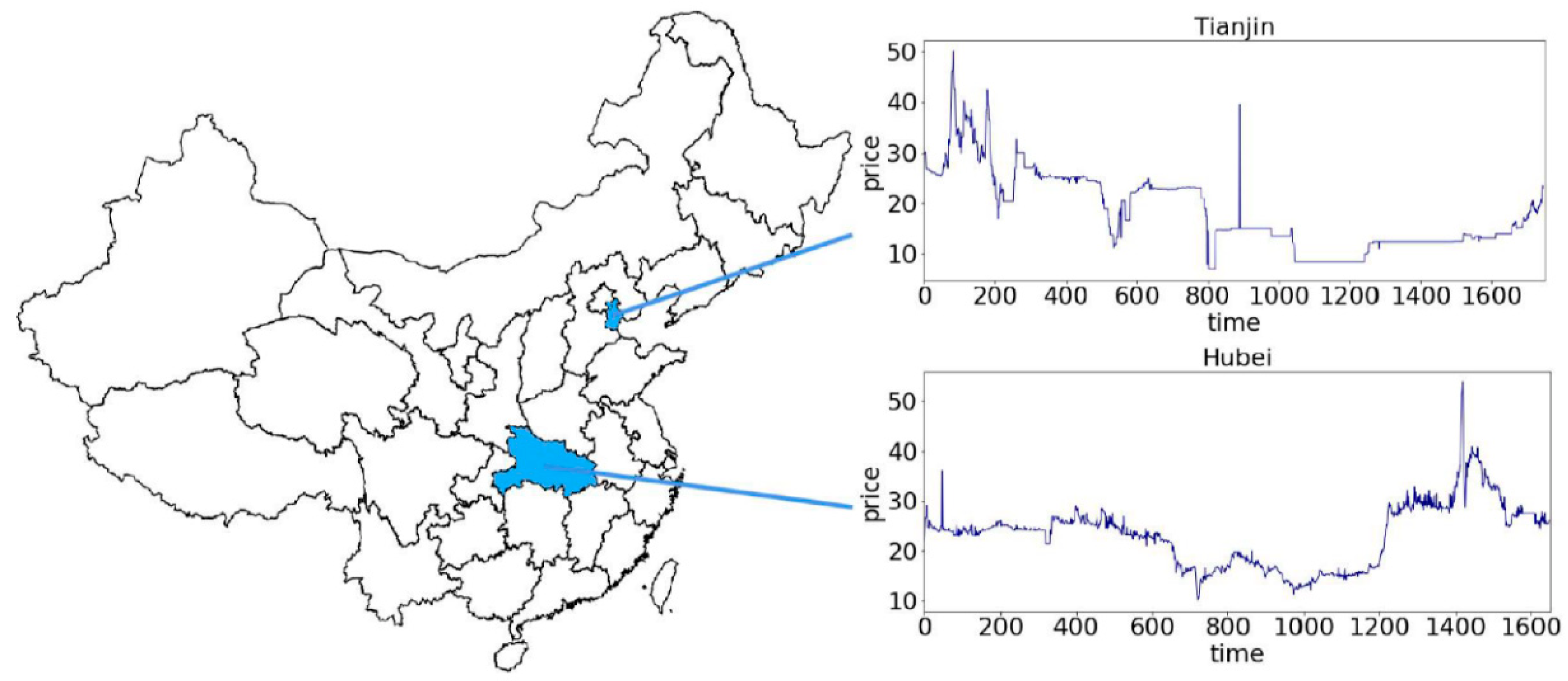
4.1. Data Collection

Carbon pricing is a tool to reduce greenhouse gas emissions. It can record the external costs of greenhouse gas emissions, that is, the publicly paid emissions costs. These costs will be revealed by pricing carbon dioxide emissions. This pricing method helps to transfer the burden of damage caused by greenhouse gas emissions to those responsible, or those who can reduce carbon dioxide emissions. Carbon pricing is not about deciding where and how to reduce emissions, but to provide economic signals to the emitters and allow them to decide to change their activities and reduce their emissions, or to continue to emit but pay for their emissions. In this way, global environmental goals can be achieved in the most flexible and cost-effective manner.

In this study, carbon trading closing price samples from Tianjin China, Hubei China, which are seen as the case 1 and case 2 independently, are selected to carry out the case study. Figure 3 shows the location of the markets and the general view. All the data can be found from the public official website: www.tanjiaoyi.com (accessed on 18 September 2021).

The time range of Tianjin China is from 26 December 2013 to 10 April 2020 and the time range of Hubei China market is from 2 April 2014 to 10 April 2020. Meanwhile, for each case study, the first 75% of the samples are treated as the training set, the last 25% act as the predicting set. Here, the samples are split according to time rather than split randomly, that is because in order to maintain the characteristics of the time series, it is necessary that the data set is segmented according to time, and this is also helpful to maintain the continuity of the time series.

4.2. Evaluation Criteria

In this study, five measures including mean absolute error (MAE), root mean squared error (RMSE), mean absolute percentage error (MAPE), coverage probability (CP), and mean width percentage (MWP) are adopted to assess the predicting ability of all involved models, which are listed in

Table 1. The statistical measurements used in the prediction results.

Error Criteria	Definition	Equation
MAE	Mean absolute error	$\frac{1}{n_1}{\displaystyle \sum _{t=1}^{n_1}\left|x(t)-\widehat{x}(t)\right|}$
RMSE	Root mean square error	$\sqrt{\frac{1}{n_1}{\displaystyle \sum _{t=1}^{n_1}{(x(t)-\widehat{x}(t))}^2}}$
MAPE	Mean absolute percentage error	$\frac{1}{n_1}{\displaystyle \sum _{t=1}^{n_1}\left|\frac{x(t)-\widehat{x}(t)}{x(t)}\right|}\times 100\%$
MWP	Mean width percentage	$\frac{1}{N}{\displaystyle \sum _{i=1}^N\frac{U(x_i)-L(x_i)}{y_i}}$
CP	Coverage probability	$\frac{{\zeta }^{1-\alpha }}{N}\times 100\%$

. Generally, the smaller the values of MAE, RMSE, MAPE, and MWP, the better the prediction ability is. While for CP, the value cannot be too large, which will reduce certainty; or too small, which will lose the significance of interval prediction.

Where $n_1$ denotes the number of prediction samples, $x(t)$ is the actual price value at time $t$ and $\widehat{x}(t)$ is the prediction value of the price at the same time point, N is the number of samples, ζ^1−α is the number of actual values that fall within the interval at confidence $1-\alpha$, $U(x_i)$ is the upper bound of the $i-th$ sample, $L(x_i)$ is the lower bound of the $i-th$ sample, $y_i$ is the $i-th$ real value.

4.3. Point Prediction

4.3.1. Case I: Test with Closing Price from Tianjin Market

This section shows the process of the first experiment whose samples are from Tianjin market. According to the introduction above, the first 75% of the samples are treated as the training set, the next 25% of the samples are the testing set.

For the initial dataset, VMD is applied to carry out the decomposition task. The dataset is divided into 13 sub-sequences, however, some of the sub-sequences can be the noise and some may contain similar features, therefore, SE calculation is applied to see whether we can combine some of them together to avoid the problem of carrying out research on similar sub-sequences. By comparing the SE value of each sub-sequence, groups with similar SE values are put together. Figure 4 shows the process described above, in particular, the values are divided into four categories: [0,0.025), [0.025,0.05), [0.05,0.15), and [0.15, +$\infty$), which means there are four sub-sequences. The selection of interval endpoints can be done through the overall SE value distribution and there are no strict requirements or rules here. The main idea is to put together sub-sequences with similar characteristics, which can simplify the following operations and improve efficiency.

Then, for each sub-sequence, random forest is carried out to form the sub-results. Each subgroup carries certain kind of the trend of the initial data series, to modify the trend to the greatest degree, random forest needs to be carried out separately in each sub-sequence. When the sub-results of each sub-sequence are obtained, LSTM is applied to integrate these four results into one which can be seen as the first prediction result. However, the result still has room for improvement where the focus goes on to the residual part. First, white noise test is carried out on the residual series, the result is shown in

Table 2. Q-value of each lag order.

Lag Order	1	2	3	4	5	6	7	8	9	10	11	12
Q-value	53.77	69.83	89.75	109.92	124.32	133.41	143.91	153.78	162.8	168.49	172.72	177.45
${\chi }_{0.95}^2\left(\mathrm{m}\right)$	0.004	0.10	0.35	0.71	1.15	1.64	2.17	2.73	3.33	3.94	4.58	5.23

.

The Q-values of each lag order are greater than the corresponding quantile value, it is obvious to see that the residual series is not a white noise series so it is meaningful to carry out residual correction process. The residual will be the input of LSTM which will generate the result. This result will be added back to the former result and this will be the final point prediction. Figure 5 shows the process and the comparison.

Meanwhile, three statistical measures are also calculated to demonstrate the predicting ability of the proposed model in experiment 1 which is shown in the following section. The parameters used in this dataset are shown in

Table 3. Parameters used in case 1.

Random Forest	LSTM Integration					LSTM Residual Correction
Min Samples Split	Batch Size	Neure	Look Back	Dropout	Seed	Batch Size	Neure	Look Back	Dropout	Seed
2	30	5	2	0.001	5	30	10	2	0.1	8

.

For the parameters used, some brief descriptions are also made here. In random forest, min sample split represents the minimum number of samples required to split internal nodes; in LSTM, batch size represents the number of samples selected for one training, neure is the number of neurons, look back affects the number of sample of the output sequence, dropout represents the probability (when it is equal to 0, it means that no dropout operation is performed), and seed affects the selection of the initial value of the parameters and the feedback of the previous training result.

4.3.2. Case II: Test with Closing Price from Hubei Market

This section studies another set of samples from the Hubei market. The process is the same with experiment 1. The initial data series is first divided into 16 subgroups. As is known to all, different data sets mean different features and characteristics, so if the number of subgroups is the same in all datasets, it is equivalent to defaulting that different data sets have similar trend characteristics, which is also unscientific. So, in case 2, the number of subgroup will not be the same as in case 1.

By comparing the SE value of each sub-sequence, the number of sub-sequence is 5 which is shown in Figure 6 where values are divided into five groups: [0,0.02), [0.02,0.05), [0.05,0.1), [0.1,0.5), and [0.5,+$\infty$).

For each sub-sequence, random forest is applied to form the sub-results which will be the input of LSTM integration. When the first result is obtained, residual can be obtained comparing with the real value. White noise test is carried out as well and the result is shown in

Table 4. Q-value of each lag order.

Lag Order	1	2	3	4	5	6	7	8	9	10	11	12
Q-value	119.80	214.40	282.29	331.73	345.77	349.61	351.19	356.08	364.69	369.37	378.43	388.16
${\chi }_{0.95}^2\left(\mathrm{m}\right)$	0.004	0.10	0.35	0.71	1.15	1.64	2.17	2.73	3.33	3.94	4.58	5.23

.

Clearly, none of the values are equal to or smaller than the corresponding quantile value, the residual series is not a white noise series which calls for residual correction. For the residual part, LSTM is applied to form the prediction result of the residual which will be added back to the first result. Then, the final result is obtained as is shown in Figure 7. In the picture shown, the comparison of residual from LSTM integration and the final residual proves that the residual correction process is necessary.

The statistical measures are also calculated and they are shown in the following section. The parameters in case 2 are shown in

Table 5. Parameters used in case 2.

Random Forest	LSTM Integration					LSTM Residual Correction
Min Samples Split	Batch Size	Neure	Look Back	Dropout	Seed	Batch Size	Neure	Look Back	Dropout	Seed
2	60	3	2	0.001	2	30	5	2	0.1	2

.

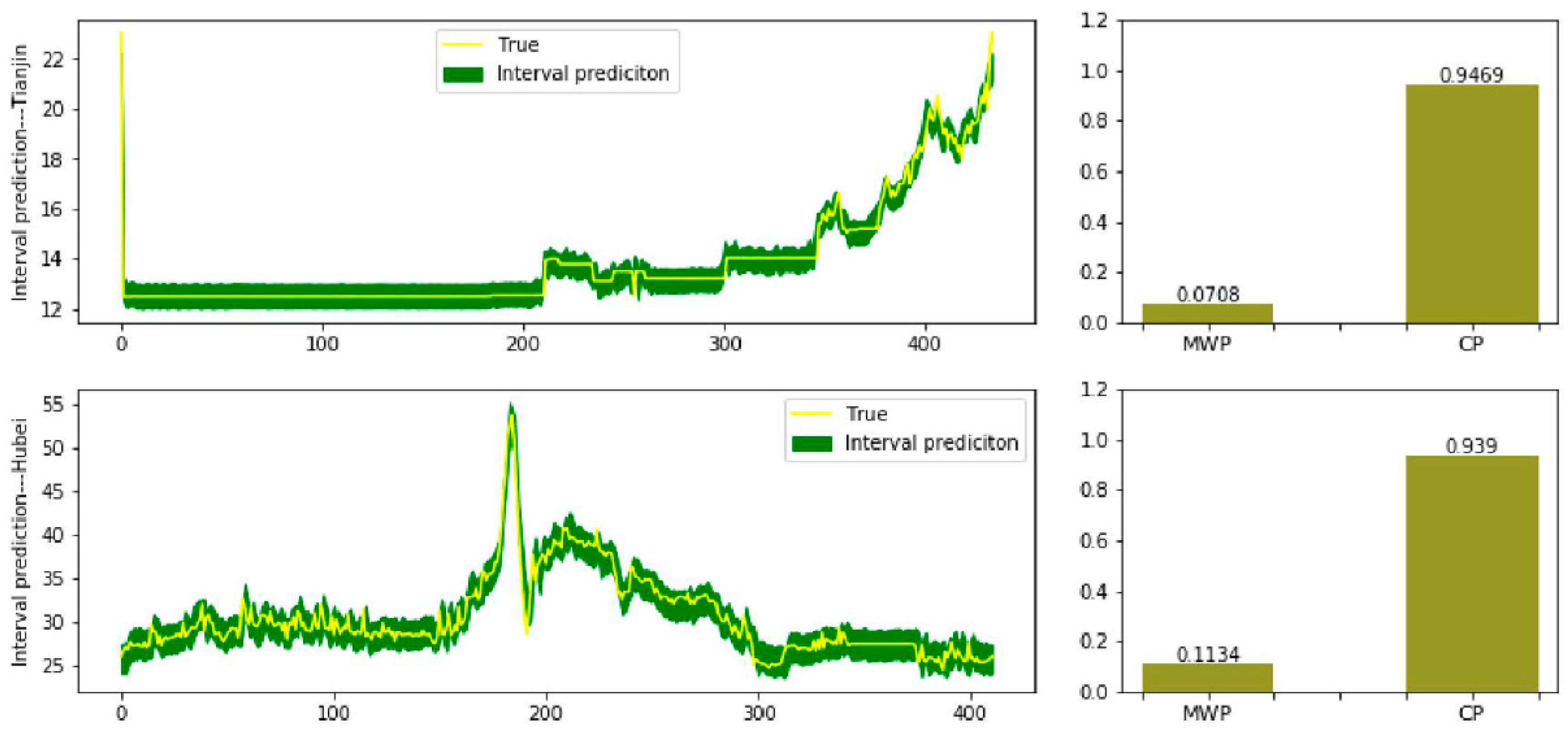
4.4. Interval Prediction

GP is carried out when the point prediction is finished to generate the interval prediction estimate. Figure 8 shows the GP result of the two cases above and the related estimation measures. The parameters used in the cases are shown in

Table 6. Parameters used in cases.

Case Name	GP Parameters
	Mean	Cov	Lik
Case 1	1	3,1,2	−1
Case 2	1	3,2,1	−2

.

Table 7. Measures of models.

Model	Case	Measure
		RMSE	MAE	MAPE	CP	MWP
Proposed Model	Tianjin	0.003	0.001	0.95%	0.95	0.07
	Hubei	0.012	0.01	2.70%	0.94	0.11
One-step BP	Tianjin	0.05	0.05	35.47%	/	/
	Hubei	0.10	0.09	30.25%	/	/
One-step random forest	Tianjin	0.03	0.02	11.68%	/	/
	Hubei	0.02	0.02	7.90%	/	/
One-step LSTM	Tianjin	0.05	0.03	11.60%	/	/
	Hubei	0.06	0.04	16.47%	/	/
Random forest -two-stage LSTM-GP	Tianjin	0.02	0.02	13.71%	1	4.07
	Hubei	0.05	0.04	14.78%	0.30	0.01
VMD-SE-random forest -one-stage LSTM-GP	Tianjin	0.003	0.002	1.79%	1	4.18
	Hubei	0.01	0.01	2.74%	0.08	0.01

shows the measures of the two cases above to demonstrate the point prediction ability of the proposed model. Meanwhile, the measures of GP are also shown in Table 7 to prove the accuracy of the interval estimate prediction.

5. Comparison Model and Discussion

5.1. Comparison Model

In this section, to further demonstrate the ability of each model, different experiments are carried out: (1) back propagation algorithm (BP), random forest, long-short term memory (LSTM) are applied separately to demonstrate the predicting ability of random forest and LSTM, this experiment also shows the performance of one-step nonlinear integration models; (2) as the proposed model applies the decomposition and feature reconstruction process, it is necessary to see without it, what performance will be provided, so the VMD-SE process is eliminated, the original dataset is the input, then random forest and LSTM are applied as the integration tools; still, LSTM also corrects the residual; (3) residual is always ignored, which is why the proposed model applied the residual correction strategy, to show its significance, VMD-SE-random forest-LSTM model which eliminates the residual correction process is applied, by comparing the performance, we can prove the importance of the residual correction.

The measures of the models mentioned above are shown in Table 7, meanwhile, the measures of the proposed model are also displayed.

5.2. Discussion

As is seen from Section 5.1, a few conclusions can be drawn:

(1)

To start with, the prediction ability of three nonlinear integration tools: BP, random forest, and LSTM are compared together especially to demonstrate the accuracy in point prediction. Seen from the table, BP does have satisfying predicting ability in that though the MAE of two cases are 0.05, 0.09 separately, no larger than 0.1, other measures, RMSE and MAPE, are far from satisfaction. While for random forest and LSTM, not only are their RMSE values below 0.1, but their MAPE values are also controlled under 20%. More specifically, the MAPE of BP in the two cases are 35.47% and 30.25%, random forest can reduce them to 11.68% and 7.9%. Even though the predicting ability of LSTM is relatively weaker than random forest, but compared to BP, LSTM can still reduce the MAPE values by 23.87% and 13.78%. Meanwhile, this experiment can still prove the accuracy of nonlinear integration methods. So, it is suitable for the proposed model to include random forest and LSTM.

(2)

Focusing on the first three experiments, when we have found out that BP shows the worst performance, it needs to be seen what differences do they have compared to the proposed model. The three single model applies the one-step nonlinear integration while the proposed model uses the two-step nonlinear integration. Seen from the results, clearly, the predicting ability shows great difference. In case 1, MAPE value goes up by 34.52%, 10.73%, and 10.65% in the one-step BP, one-step random forest, and one-step LSTM. This is the same in case 2, MAPE value inclines by 11.2 times, 2.93 times and 6.1 times separately. Meanwhile, RMSE and MAE values are affected. Only the proposed model can control them under 0.01 in case 1 and 0.015 in case 2. For certain, the accuracy of simple one-step nonlinear integration is not that bad (MAPE in case 2 of one-step random forest), however, we cannot be too careful when it comes to the precise prediction. That is why this paper applies the two-step nonlinear integration.

(3)

Then, many existing studies usually carry out research on the original dataset without decomposition or feature reconstruction. In the proposed model, these two jobs are realized by the VMD-SE process; so, the second experiment eliminates VMD-SE process to prove the significance of decomposition and feature reconstruction. Drawn from the table, RMSE, MAE, and MAPE values show increases, the RMSE value in case 2 is four times and more, MAE value in case 1 is 20 times the value of the proposed model’s; for MAPE values, they increase by 12.76% and 12.08% separately which means the predicting ability is affected; for the interval prediction, even CP value increases in case 1, but for the MWP value of it, the value is 58 times larger, which means the interval contains more uncertainty; while in case 2, CP value shows a great decrease even if MWP value is satisfying, this means even the interval is reliable in some way, the sample point is not in the interval which is meaningless to study the interval. Thus, it is beyond argument that the decomposition or feature reconstruction process can obviously raise the predicting accuracy which means the arrangement of the proposed model is more reliable.

(4)

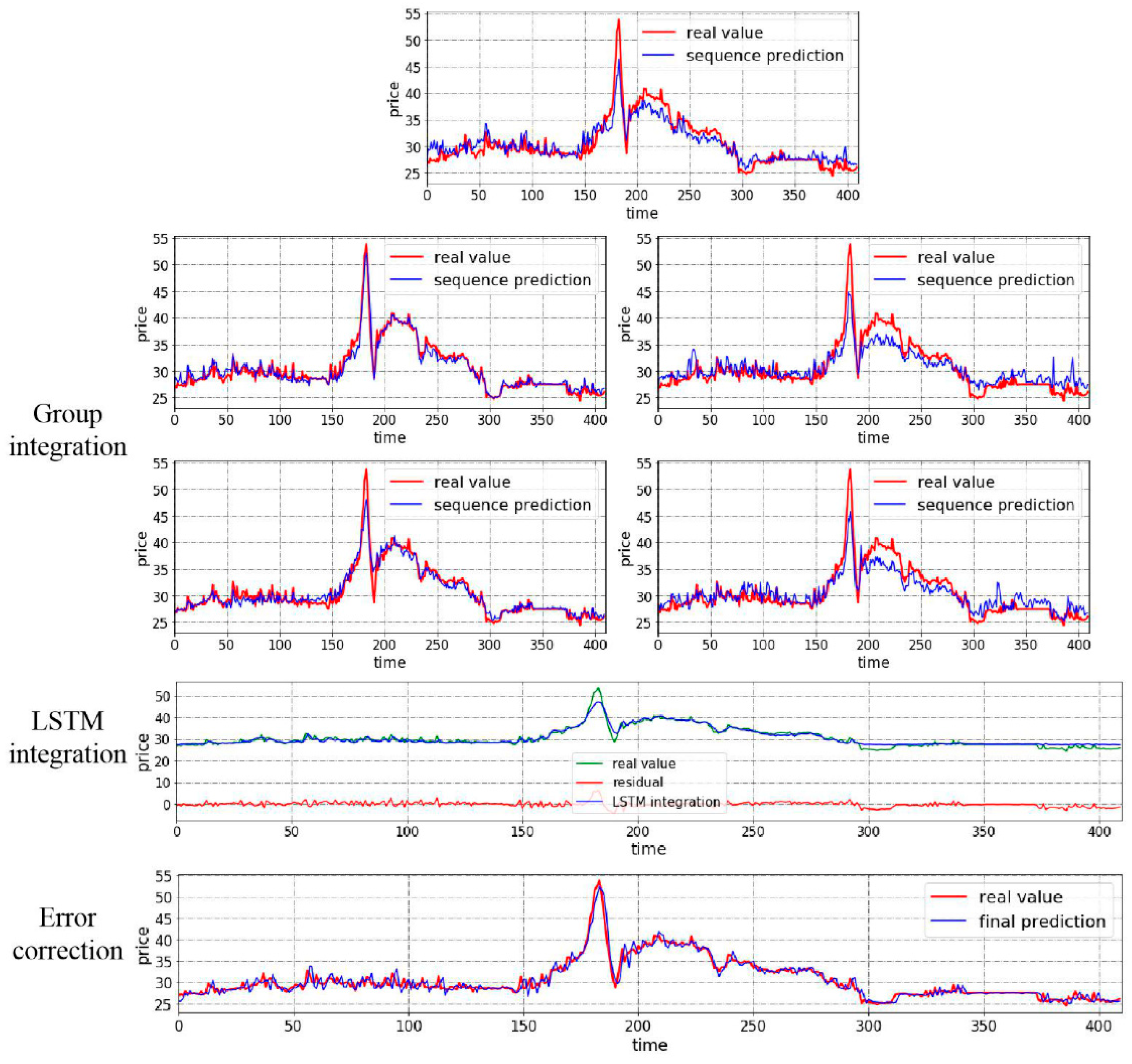
In the meantime, the third experiment is carried out to demonstrate the significance of residual correction. In the VMD-SE-random forest-LSTM model, the residual correction process is eliminated. RMSE and MAE values in the two cases show no great differences but, apparently, MAPE value goes higher in case 1, increased by 0.84%. This means the residual contains much unextracted information. For the interval prediction, CP values even though show a slight increase in case 1, however, what needs to be emphasized is the MWP value. It has been stressed above that MWP stands for the width of the interval, larger MWP value means the interval is bigger which is not the best interval estimate, that is, the gap is too wide to lower the fault tolerance to show the decline of uncertainty. The MWP value is 59 more times larger than that in the proposed model in case 1. Then, it may seem to be performing well in the point prediction of case 2, but like in the last experiment, CP value is disappointing, which goes down by 0.86, losing the significance of interval prediction. Many existing works will usually tend to ignore the residual series, however, doing this means even there is valuable information in the residual series, the information will not be paid attention to. That is why this paper focuses on the residual as well, showing effort to grasp the information as much as possible, making the whole process of the proposed model more persuasive.

From all the experiments above, the results show vividly the reason of model choice as well as the importance of two-step nonlinear integration, decomposition-feature reconstruction system and residual correction. The proposed model pays to much attention to the details that are easy to be neglected; drawn from the results, the prediction accuracy is satisfying and the intervals are suitable.

6. Conclusions

In this study, an optimal multi-scale nonlinear ensemble model is proposed to predict the carbon trading price in two different markets. The proposed decomposition and feature reconstruction system, which contains VMD and SE, not only carries out the decomposition job but also the feature reconstruction work. Then, the nonlinear methods including random forest and LSTM are applied for prediction and integration, also this process is seen as a two-step nonlinear integration process. The residual part is also given attention, after it is confirmed not to be a white noise series, it will be added back when LSTM correction is finished to generate the final result. Then proposed model also generates the prediction interval estimate via GP which increases the fault tolerance and decreases the uncertainty.

The proposed model combines different kinds of machine learning methods and in the meantime, the advantages of each method are used to a large extent. Moreover, the proposed model can be applied not only in the field of carbon price prediction but also other field such as data prediction or trend modification. Moreover, the methods included have some space for improvements, for instance, some other decomposition methods can replace the method in the proposed model.

References

1. Fan, J.; Todorova, N. Dynamics of China’s carbon prices in the pilot trading phase. Appl. Energy 2017, 208, 1452–1467. [Google Scholar] [CrossRef] [Green Version]
2. Ivanovski, K.; Churchill, S. Convergence and determinants of greenhouse gas emissions in Australia: A regional analysis. Energy Econ. 2020, 92, 104971. [Google Scholar] [CrossRef]
3. Chao, Q.; Yongrok, C. A study on the CO2 marginal abatement cost of coal-fueled power plants: Is the current price of China pilot carbon emission trading market rational? Carbon Manag. 2020, 11, 303–314. [Google Scholar]
4. Fang, C.; Ma, T. Stylized agent-based modeling on linking emission trading systems and its implications for China’s practice. Energy Econ. 2020, 92, 104916. [Google Scholar] [CrossRef]
5. Yu, X.; Dong, Z.; Zhou, D.; Sang, X.; Chang, C.; Huang, X. Integration of tradable green certificates trading and carbon emissions trading: How will Chinese power industry do? J. Clean. Prod. 2021, 279, 123485. [Google Scholar] [CrossRef]
6. Liu, H.; Shen, L. Forecasting carbon price using empirical wavelet transform and gated recurrent unit neural network. Carbon Manag. 2019, 11, 25–37. [Google Scholar] [CrossRef]
7. Zhu, B.; Han, D.; Wang, P.; Wu, Z.; Zhang, T.; Wei, Y. Forecasting carbon price using empirical mode decomposition and evolutionary least squares support vector regression. Appl. Energy 2017, 191, 521–530. [Google Scholar] [CrossRef] [Green Version]
8. Qin, Q.; He, H.; Li, L.; He, L. A Novel Decomposition-Ensemble Based Carbon Price Forecasting Model Integrated with Local Polynomial Prediction. Comput. Econ. 2020, 55, 1249–1273. [Google Scholar] [CrossRef]
9. Tian, C.; Hao, Y. Point and interval forecasting for carbon price based on an improved analysis-forecast system. Appl. Math. Model. 2020, 79, 126–144. [Google Scholar] [CrossRef]
10. Sun, W.; Zhang, C.; Sun, C. Carbon pricing prediction based on wavelet transform and K-ELM optimized by bat optimization algorithm in China ETS: The case of Shanghai and Hubei carbon markets. Carbon Manag. 2018, 9, 605–617. [Google Scholar]
11. Wu, Q.; Liu, Z. Forecasting the carbon price sequence in the Hubei emissions exchange using a hybrid model based on ensemble empirical mode decomposition. Energy Sci. Eng. 2020, 8, 2708–2721. [Google Scholar] [CrossRef] [Green Version]
12. Sun, W.; Sun, C.; Li, Z. A Hybrid Carbon Price Forecasting Model with External and Internal Influencing Factors Considered Comprehensively: A Case Study from China. Pol. J. Environ. Stud. 2020, 29, 3305–3316. [Google Scholar] [CrossRef]
13. Huang, Y.; He, Z. Carbon price forecasting with optimization prediction method based on unstructured combination. Sci. Total Environ. 2020, 725, 138350. [Google Scholar] [CrossRef]
14. Liu, Y.; Yang, G.; Li, M.; Yin, H. Variational mode decomposition denoising combined the detrended fluctuation analysis. Signal Process 2016, 125, 349–364. [Google Scholar] [CrossRef]
15. Sun, W.; Huang, C. A carbon price prediction model based on secondary decomposition algorithm and optimized back propagation neural network. J. Clean. Prod. 2020, 243, 118671. [Google Scholar] [CrossRef]
16. Zhu, J.; Wu, P.; Chen, H.; Liu, J.; Zhou, L. Carbon price forecasting with variational mode decomposition and optimal combined model. Phys. A 2019, 519, 140–158. [Google Scholar] [CrossRef]
17. Singh, S.N.; Mohapatra, A. Repeated wavelet transform based ARIMA model for very short-term wind speed forecasting. Renew. Energy 2019, 136, 758–768. [Google Scholar]
18. Mbah, T.J.; Ye, H.W.; Zhang, J.H.; Long, M. Using LSTM and ARIMA to Simulate and Predict Limestone Price Variations. Min. Met. Explor. 2021, 38, 913–926. [Google Scholar]
19. Zhang, J.; Li, D.; Hao, Y.; Tan, Z. A hybrid model using signal processing technology, econometric models and neural network for carbon spot price forecasting. J. Clean. Prod. 2018, 204, 958–964. [Google Scholar] [CrossRef]
20. Dutta, A. Modeling and forecasting the volatility of carbon emission market: The role of outliers, time-varying jumps and oil price risk. J. Clean. Prod. 2018, 172, 2773–2781. [Google Scholar] [CrossRef]
21. Sanin, M.E.; Violante, F.; Mansanet-Bataller, M. Understanding volatility dynamics in the EU-ETS market. Energy Policy 2018, 82, 321–331. [Google Scholar] [CrossRef] [Green Version]
22. Zeitlberger, A.; Brauneis, A. Modeling carbon spot and futures price returns with GARCH and Markov switching GARCH models: Evidence from the first commitment period (2008–2012). Cent. Eur. J. Oper. Res. 2016, 1, 149–176. [Google Scholar] [CrossRef]
23. Zainuddin, N.; Lola, M.; Djauhari, M.; Yusof, F.; Ramlee, M.; Deraman, A.; Ibrahim, Y.; Abdullah, M. Improvement of time forecasting models using a novel hybridization of bootstrap and double bootstrap artificial neural networks. Appl. Soft Comput. 2019, 84, 105676. [Google Scholar] [CrossRef]
24. Jamous, R.; ALRahhal, H.; El-Darieby, M. A New ANN-Particle Swarm Optimization with Center of Gravity (ANN-PSOCoG) Prediction Model for the Stock Market under the Effect of COVID-19. Sci. Program. 2021, 2021, 6656150. [Google Scholar]
25. Liu, W.P.; Wang, C.Z.; Li, Y.G.; Liu, Y.S.; Huang, K.K. Ensemble forecasting for product futures prices using variational mode decomposition and artificial neural networks. Chaos Soliton Fractals 2021, 146, 110822. [Google Scholar] [CrossRef]
26. Wen, L.; Liu, Y. A Research about Beijing’s Carbon Emissions Based on the IPSO-BP Model. Environ. Prog. Sustain. Energy 2017, 36, 428–434. [Google Scholar] [CrossRef]
27. Yu, R.; Gao, J.; Yu, M.; Lu, W.; Xu, T.; Zhao, M.; Zhang, J.; Zhang, R.; Zhang, Z. LSTM-EFG for wind power forecasting based on sequential correlation features. Futur. Gener. Comp. Syst. 2019, 93, 33–42. [Google Scholar] [CrossRef]
28. Han, M.; Ding, L.; Zhao, X.; Kang, W. Forecasting carbon prices in the Shenzhen market, China: The role of mixed-frequency factors. Energy 2019, 171, 69–76. [Google Scholar] [CrossRef]
29. Wei, S.; Wang, T.; Li, Y. Influencing factors and prediction of carbon dioxide emissions using factor analysis and optimized least squares support vector machine. Environ. Eng. 2017, 22, 175–185. [Google Scholar] [CrossRef]
30. Qiao, W.; Lu, H.; Zhou, G.; Azimi, M.; Yang, Q.; Tian, W. A hybrid algorithm for carbon dioxide emissions forecasting based on improved lion swarm optimizer. J. Clean. Prod. 2020, 244, 118612. [Google Scholar] [CrossRef]
31. Zhu, B.; Ye, S.; Wang, P.; He, K.; Zhang, T.; Wei, Y. A novel multiscale nonlinear ensemble leaning paradigm for carbon price forecasting. Energy Econ. 2018, 70, 143–157. [Google Scholar] [CrossRef]
32. Wen, L.; Cao, Y. Influencing factors analysis and forecasting of residential energy-related CO2 emissions utilizing optimized support vector machine. J. Clean. Prod. 2020, 250, 119492. [Google Scholar] [CrossRef]
33. Fan, Y.Q.; Sun, Z.H. CPI Big Data Prediction Based on Wavelet Twin Support Vector Machine. Int. J. Pattern Recogn. 2021, 35, 2159013. [Google Scholar] [CrossRef]
34. Athey, S.; Tibshirani, J.; Wager, S. Generalized Random Forests. Ann. Stat. 2019, 47, 1148–1178. [Google Scholar] [CrossRef] [Green Version]
35. Lu, H.; Ma, X.; Huang, K.; Azimi, M. Carbon trading volume and price forecasting in China using multiple machine learning models. J. Clean. Prod. 2020, 249, 119386. [Google Scholar] [CrossRef]
36. Sun, Q. Research on the driving factors of energy carbon footprint in Liaoning province using Random Forest algorithm. Appl. Ecol. Environ. Res. 2019, 17, 8381–8394. [Google Scholar] [CrossRef]
37. Wen, L.; Yuan, X. Forecasting CO2 emissions in Chinas commercial department, through BP neural network based on random forest and PSO. Sci. Total Environ. 2020, 718, 137194. [Google Scholar] [CrossRef]
38. Sharaf, M.; Hemdan, E.E.; El-Sayed, A.; El-Bahnasawy, N.A. StockPred: A framework for stock Price prediction. Multimed. Tools Appl. 2021, 80, 17923–17954. [Google Scholar] [CrossRef]
39. Huang, Y.; Shen, L.; Liu, H. Grey relational analysis, principal component analysis and forecasting of carbon emissions based on long short-term memory in China. J. Clean. Prod. 2019, 209, 415–423. [Google Scholar] [CrossRef]
40. Yang, S.; Chen, D.; Li, S.; Wang, W. Carbon price forecasting based on modified ensemble empirical mode decomposition and long short-term memory optimized by improved whale optimization algorithm. Sci. Total Environ. 2020, 716, 137117. [Google Scholar] [CrossRef]
41. Yan, L. Forecasting Chinese carbon emissions based on a novel time series prediction method. Energy Sci. Eng. 2020, 8, 2274–2285. [Google Scholar]
42. Karmiani, R.; Kazi, A.; Nambisan, A.; Shah, A.; Kamble, V. Comparison of Predictive Algorithms: Backpropagation, SVM, LSTM and Kalman Filter for Stock Market. In Proceedings of the 2019 Amity International Conference on Artificial Intelligence (AICAI), Dubai, United Arab Emirates, 4–6 February 2019; Volume 2, pp. 228–234. [Google Scholar]
43. Oliver Muncharaz, J. Comparing classic time series models and the LSTM recurrent neural network: An application to S&P 500 stocks. Financ. Mark. Valuat. 2020, 6, 137–148. [Google Scholar]
44. Pan, S. Coal Price Prediction based on LSTM. J. Phys. Conf. Ser. 2021, 1802, 042055. [Google Scholar] [CrossRef]
Figure 1. The general process of LSTM.
Mathematics 09 02595 g001
Figure 2. Flowchart of the proposed model.
Mathematics 09 02595 g002
Figure 3. The location of the markets and the general view.
Mathematics 09 02595 g003
Figure 4. The VMD-SE process of case 1.
Mathematics 09 02595 g004
Figure 5. The point prediction of case 1.
Mathematics 09 02595 g005
Figure 6. The VMD-SE process of case 2.
Mathematics 09 02595 g006
Figure 7. The point prediction of case 2.
Mathematics 09 02595 g007
Figure 8. The interval prediction estimate of two cases.
Mathematics 09 02595 g008