
Genetic Feature Selection Applied to KOSPI and Cryptocurrency Price Prediction


Abstract
:1. Introduction
2. Related Work
2.1. Feature Selection
2.2. Genetic Algorithm
2.3. Stock Index Prediction
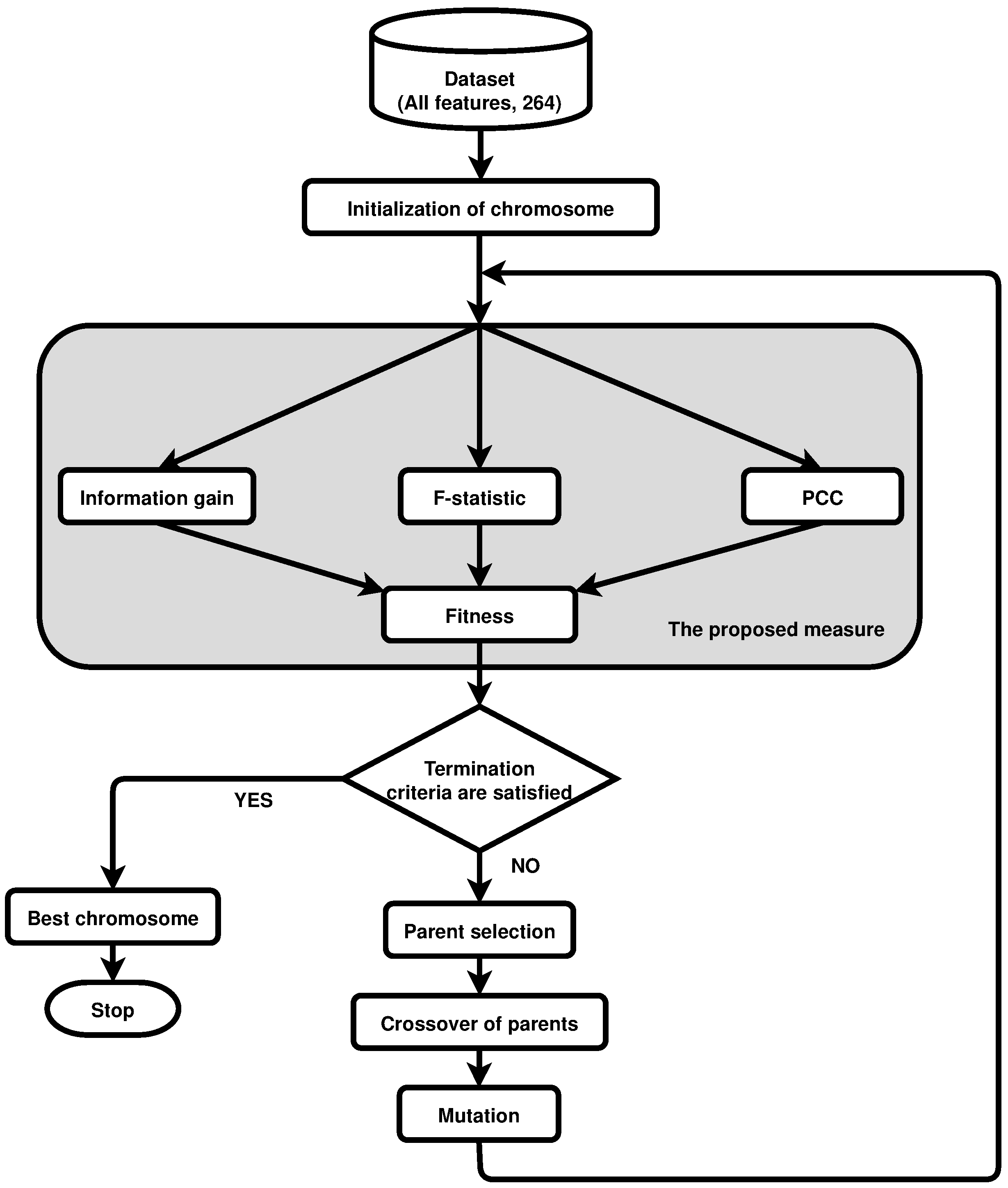
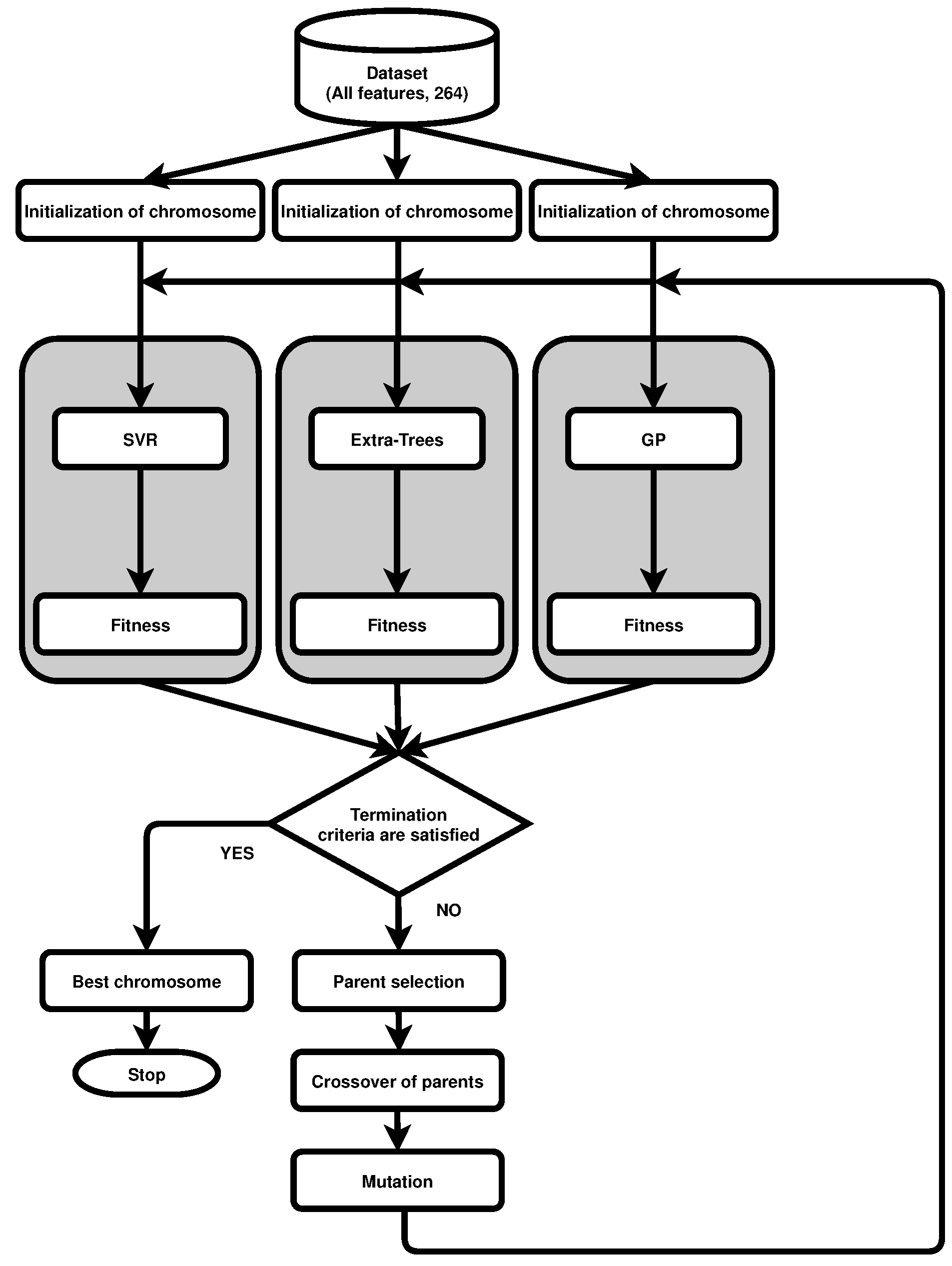
3. Genetic Algorithm for Feature Selection
3.1. Encoding and Fitness
3.2. Selection
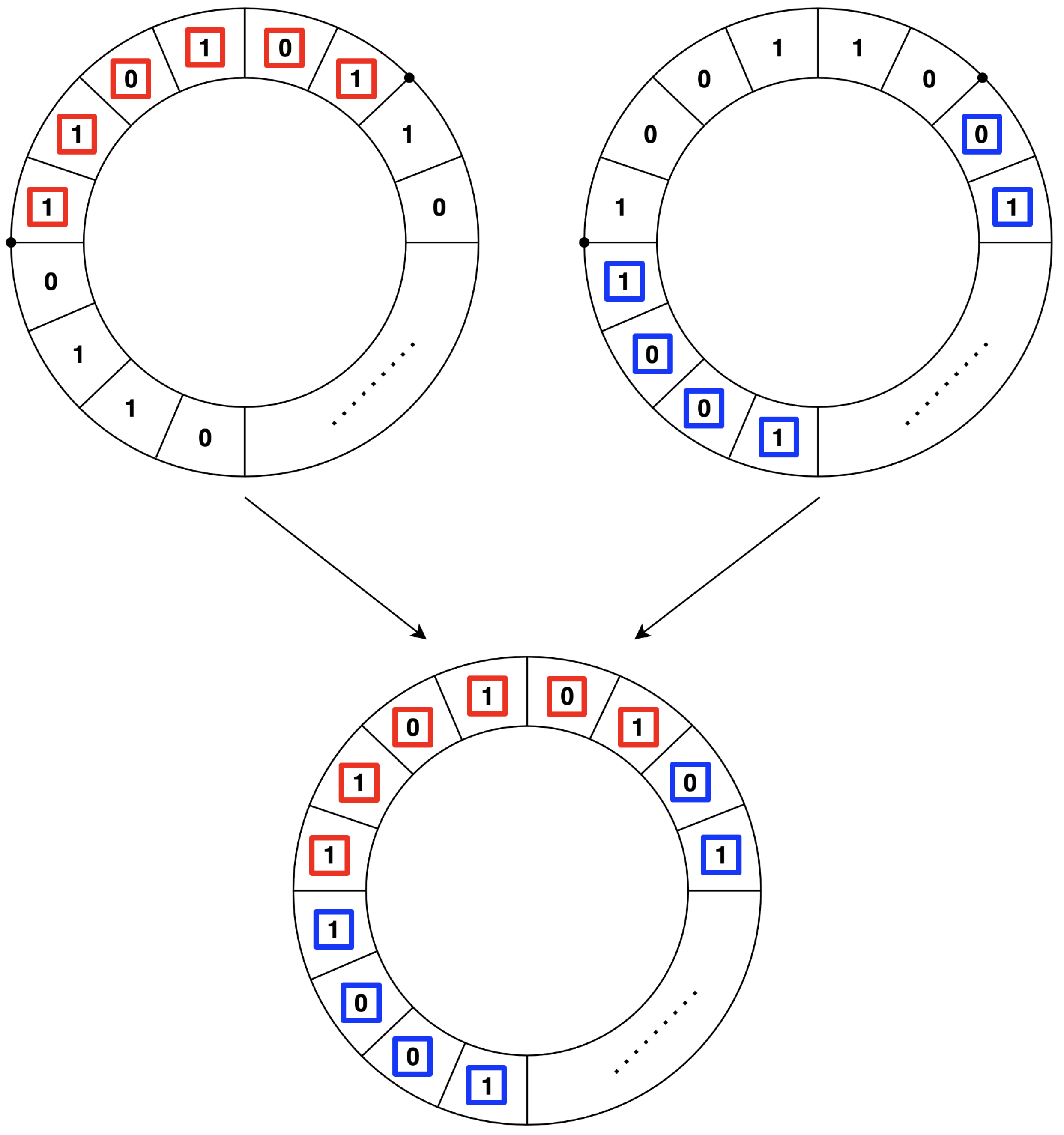
3.3. Crossover
3.4. Mutation and Replacement
3.5. Genetic Filter
3.5.1. Mutual Information
3.5.2. F-Test
3.5.3. Pearson Correlation Coefficient
3.6. Genetic Wrapper
3.6.1. Support Vector Regression
3.6.2. Extra-Trees Regression
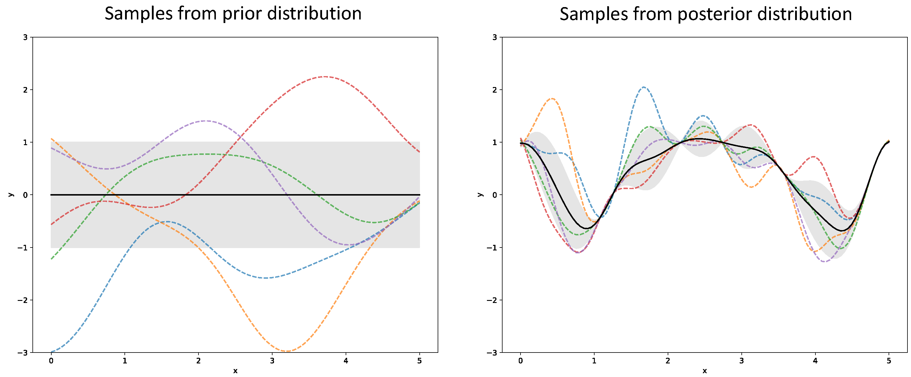
3.6.3. Gaussian Process Regression
4. Experiments and Evaluation
4.1. Experimental Setup
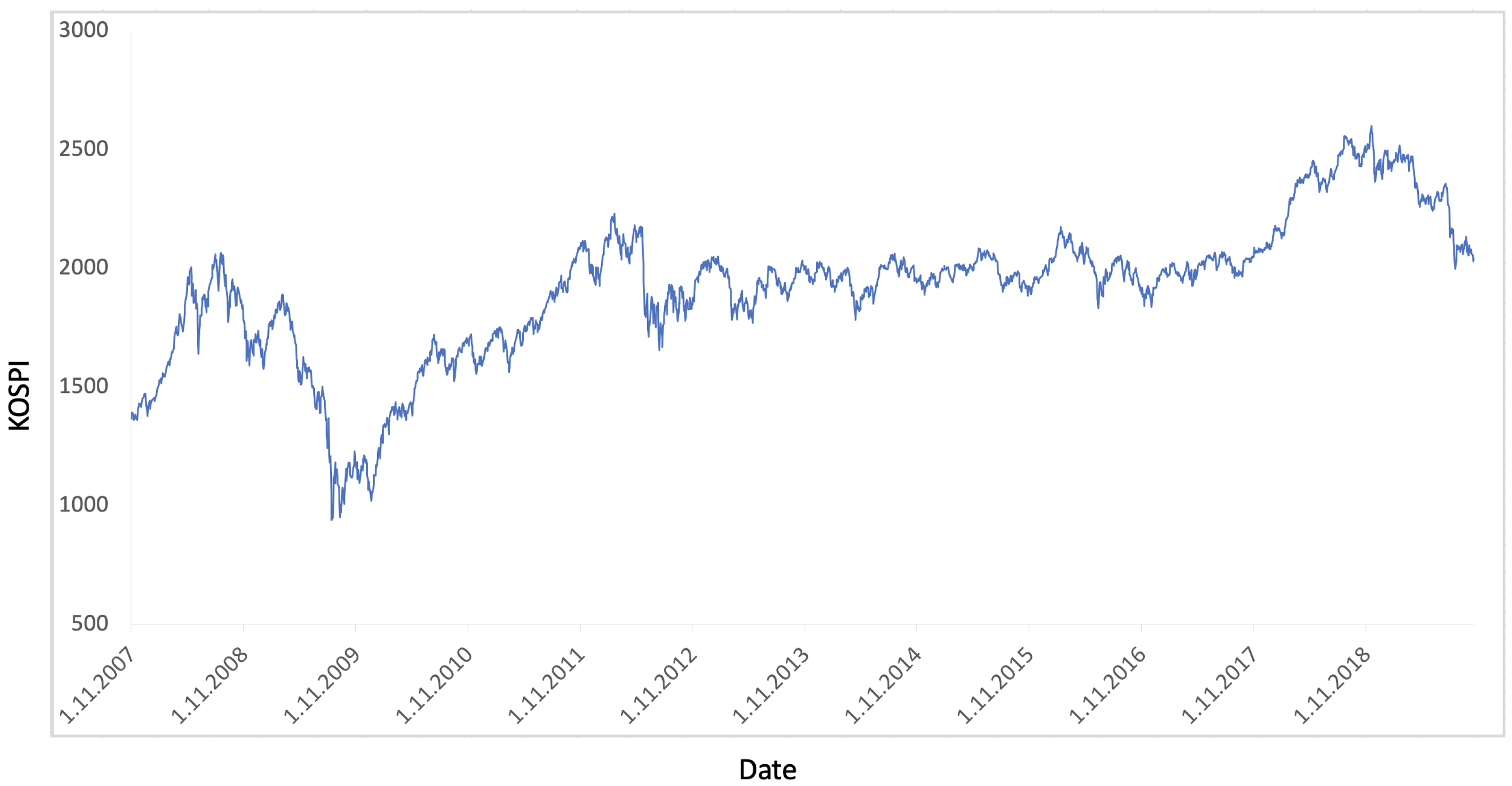
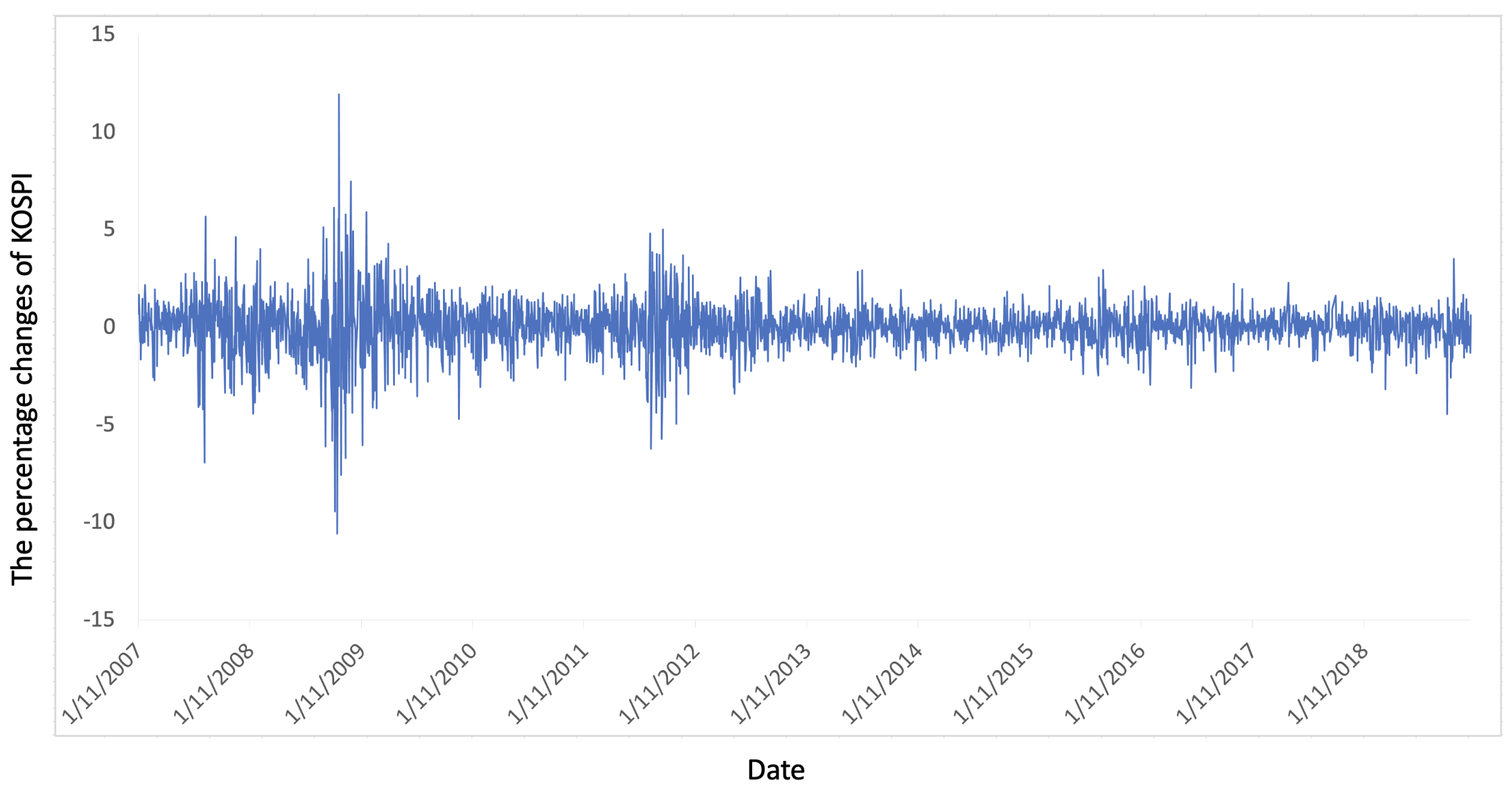
4.2. KOSPI Prediction
4.2.1. Experiment of Genetic Filter
4.2.2. Experiment of Genetic Wrapper
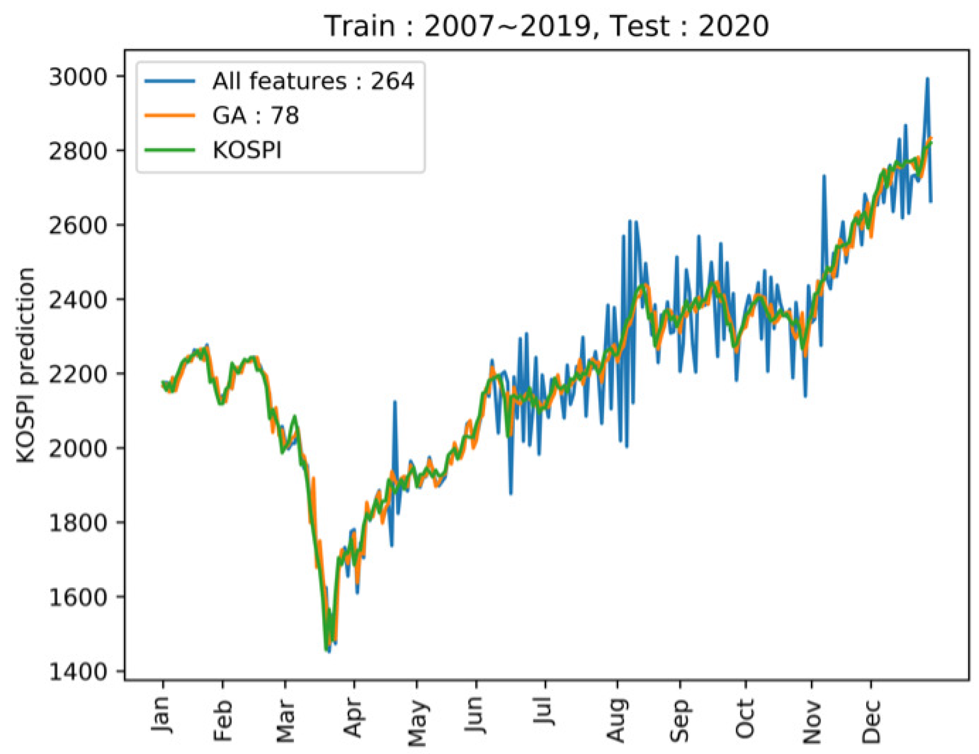
4.2.3. Prediction of KOSPI after COVID-19
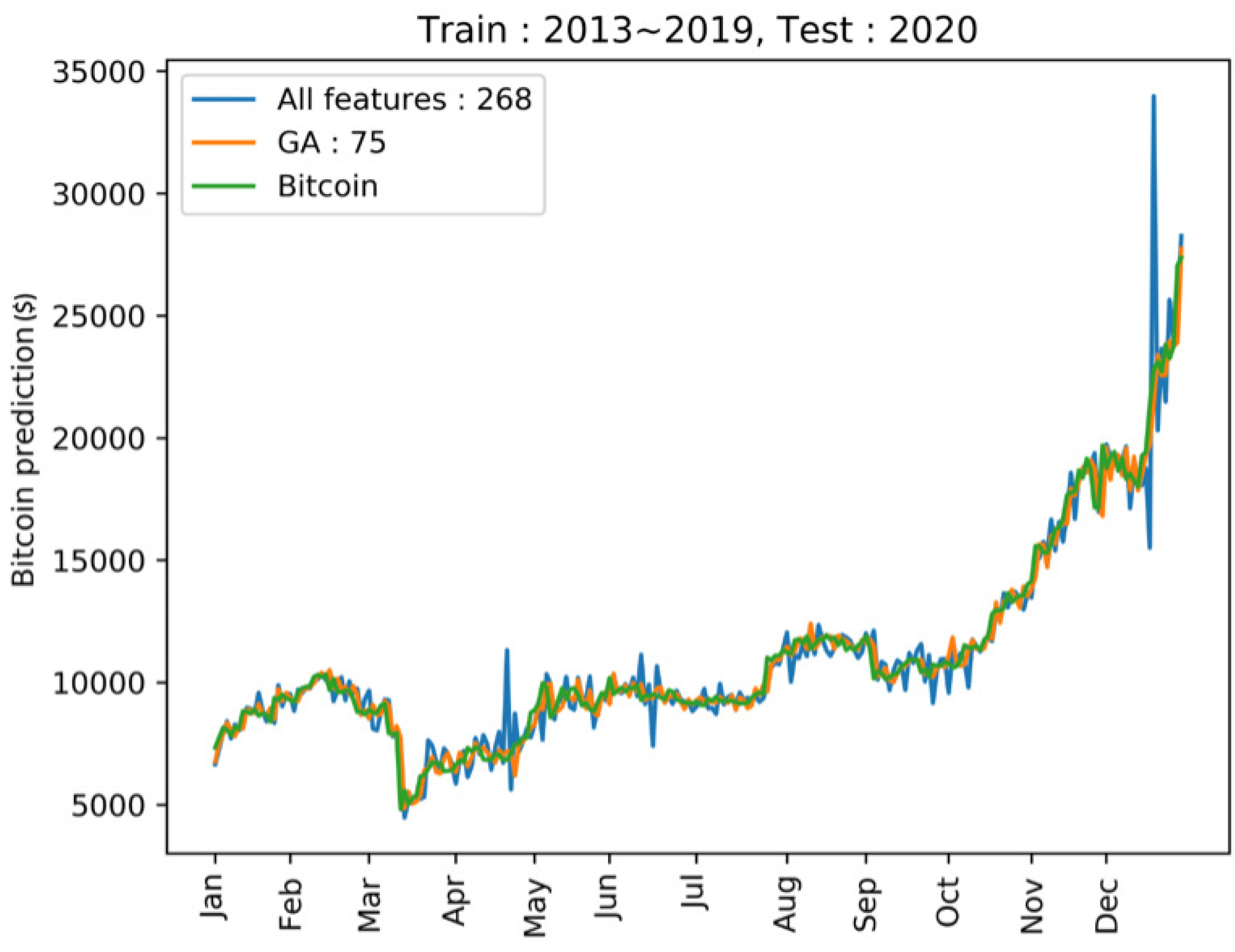
4.3. Prediction of Cryptocurrency Price and Direction
5. Conclusions
Author Contributions
Funding
Institutional Review Board Statement
Informed Consent Statement
Data Availability Statement
Conflicts of Interest
Appendix A. Results of Applying Genetic Feature Selection to Various Data

| Support Vector Regression | ||||||||||||||
|---|---|---|---|---|---|---|---|---|---|---|---|---|---|---|
| Train (year) | ’07–’08 | ’09–’10 | ’11–’12 | ’13–’14 | ’15–’16 | Average | ’07–09’ | ’10–’12 | ’13–’15 | Average | ’07–’10 | ’11–’14 | Average | |
| Test (year) | ’09–’10 | ’11–’12 | ’13–’14 | ’15–’16 | ’17–’18 | ’10–12’ | ’13–’15 | ’16–’18 | ’11–’14 | ’15–’18 | ||||
| All features | MAE | 177.766 | 314.833 | 45.645 | 51.226 | 321.983 | 182.291 | 312.076 | 89.221 | 234.325 | 211.874 | 317.419 | 200.754 | 259.086 |
| Genetic filter | MAE | 177.757 | 314.844 | 45.640 | 51.224 | 321.982 | 182.289 | 312.058 | 89.227 | 234.326 | 211.870 | 317.415 | 200.756 | 259.086 |
| Genetic wrapper | MAE | 177.755 | 314.840 | 45.639 | 51.223 | 321.975 | 182.286 | 312.035 | 89.226 | 234.316 | 211.859 | 317.411 | 200.756 | 259.083 |
| Train (year) | ’07–’09 | ’09–’11 | ’11–’13 | ’13–’15 | ’15–’17 | Average | ’07–10’ | ’10–’13 | ’13–’16 | Average | ’07–’11 | ’11–’15 | Average | |
| Test (year) | ’10 | ’12 | ’14 | ’16 | ’18 | ’11–12’ | ’14–’15 | ’17–’18 | ’12–’14 | ’16–’18 | ||||
| All features | MAE | 185.103 | 201.155 | 38.720 | 39.381 | 287.315 | 150.335 | 310.083 | 74.941 | 332.257 | 239.094 | 251.678 | 239.433 | 245.556 |
| Genetic filter | MAE | 185.080 | 201.089 | 38.713 | 39.374 | 287.311 | 150.313 | 310.068 | 74.949 | 332.264 | 239.094 | 251.559 | 239.427 | 245.493 |
| Genetic wrapper | MAE | 185.018 | 201.089 | 38.712 | 39.373 | 287.307 | 150.300 | 310.037 | 74.949 | 332.258 | 239.081 | 251.557 | 239.418 | 245.487 |
| Extra-Trees Regression | ||||||||||||||
| Train (year) | ’07–’08 | ’09–’10 | ’11–’12 | ’13–’14 | ’15–’16 | Average | ’07–09’ | ’10–’12 | ’13–’15 | Average | ’07–’10 | ’11–’14 | Average | |
| Test (year) | ’09–’10 | ’11–’12 | ’13–’14 | ’15–’16 | ’17–’18 | ’10–12’ | ’13–’15 | ’16–’18 | ’11–’14 | ’15–’18 | ||||
| All features | MAE | 165.491 | 127.589 | 66.537 | 62.434 | 232.963 | 131.002 | 260.481 | 56.035 | 246.607 | 187.708 | 108.637 | 231.505 | 170.071 |
| Genetic filter | MAE | 176.295 | 120.528 | 58.085 | 53.078 | 224.110 | 126.419 | 197.495 | 84.312 | 155.840 | 145.883 | 152.652 | 179.329 | 165.991 |
| Genetic wrapper | MAE | 165.460 | 82.843 | 47.618 | 50.715 | 214.924 | 112.312 | 94.575 | 65.917 | 154.673 | 105.055 | 66.519 | 176.728 | 121.624 |
| Train (year) | ’07–’09 | ’09–’11 | ’11–’13 | ’13–’15 | ’15–’17 | Average | ’07–10’ | ’10–’13 | ’13–’16 | Average | ’07–’11 | ’11–’15 | Average | |
| Test (year) | ’10 | ’12 | ’14 | ’16 | ’18 | ’11–12’ | ’14–’15 | ’17–’18 | ’12–’14 | ’16–’18 | ||||
| All features | MAE | 134.866 | 128.808 | 110.170 | 95.954 | 117.360 | 117.431 | 92.621 | 54.512 | 285.179 | 144.104 | 194.587 | 186.409 | 190.498 |
| Genetic filter | MAE | 140.876 | 47.645 | 49.813 | 54.896 | 151.581 | 88.962 | 142.724 | 67.217 | 215.173 | 141.705 | 141.372 | 206.220 | 173.796 |
| Genetic wrapper | MAE | 75.676 | 44.411 | 47.640 | 52.637 | 137.501 | 71.573 | 89.292 | 64.663 | 214.648 | 122.868 | 110.697 | 202.073 | 156.385 |
| Gaussian Process Regression | ||||||||||||||
| Train (year) | ’07–’08 | ’09–’10 | ’11–’12 | ’13–’14 | ’15–’16 | Average | ’07–09’ | ’10–’12 | ’13–’15 | Average | ’07–’10 | ’11–’14 | Average | |
| Test (year) | ’09–’10 | ’11–’12 | ’13–’14 | ’15–’16 | ’17–’18 | ’10–12’ | ’13–’15 | ’16–’18 | ’11–’14 | ’15–’18 | ||||
| All features | MAE | 72.135 | 167.170 | 265.885 | 137.362 | 91.568 | 146.824 | 211.181 | 405.919 | 173.120 | 263.407 | 365.998 | 155.047 | 260.522 |
| Genetic filter | MAE | 76.803 | 141.921 | 239.784 | 117.810 | 144.677 | 144.199 | 276.622 | 329.960 | 106.970 | 237.851 | 361.232 | 146.354 | 253.793 |
| Genetic wrapper | MAE | 73.758 | 134.860 | 174.954 | 117.760 | 102.760 | 120.818 | 259.285 | 143.801 | 101.354 | 168.147 | 353.156 | 128.033 | 240.594 |
| Train (year) | ’07–’09 | ’09–’11 | ’11–’13 | ’13–’15 | ’15–’17 | Average | ’07–10’ | ’10–’13 | ’13–’16 | Average | ’07–’11 | ’11–’15 | Average | |
| Test (year) | ’10 | ’12 | ’14 | ’16 | ’18 | ’11–12’ | ’14–’15 | ’17–’18 | ’12–’14 | ’16–’18 | ||||
| All features | MAE | 129.863 | 50.691 | 77.237 | 74.696 | 125.353 | 91.568 | 71.647 | 94.057 | 142.701 | 102.801 | 634.979 | 364.232 | 499.605 |
| Genetic filter | MAE | 100.722 | 65.604 | 62.663 | 72.879 | 100.608 | 80.495 | 82.995 | 65.525 | 152.018 | 100.179 | 169.793 | 189.886 | 179.839 |
| Genetic wrapper | MAE | 94.505 | 41.152 | 59.638 | 46.656 | 85.101 | 65.410 | 82.416 | 61.501 | 141.643 | 95.186 | 58.731 | 114.770 | 86.750 |
| Support Vector Regression | ||||||||||||||
|---|---|---|---|---|---|---|---|---|---|---|---|---|---|---|
| Train (year) | ’07–’08 | ’09–’10 | ’11–’12 | ’13–’14 | ’15–’16 | Average | ’07–09’ | ’10–’12 | ’13–’15 | Average | ’07–’10 | ’11–’14 | Average | |
| Test (year) | ’09–’10 | ’11–’12 | ’13–’14 | ’15–’16 | ’17–’18 | ’10–12’ | ’13–’15 | ’16–’18 | ’11–’14 | ’15–’18 | ||||
| All features | MAE | 13.960 | 19.010 | 10.509 | 11.296 | 12.964 | 13.548 | 16.843 | 10.979 | 12.158 | 13.327 | 14.869 | 12.122 | 13.495 |
| Genetic filter | MAE | 13.959 | 19.009 | 10.509 | 11.294 | 12.963 | 13.547 | 16.842 | 10.979 | 12.157 | 13.326 | 14.867 | 12.122 | 13.494 |
| Genetic wrapper | MAE | 13.959 | 19.009 | 10.508 | 11.294 | 12.963 | 13.546 | 16.841 | 10.978 | 12.157 | 13.325 | 14.867 | 12.120 | 13.493 |
| Train (year) | ’07–’09 | ’09–’11 | ’11–’13 | ’13–’15 | ’15–’17 | Average | ’07–10’ | ’10–’13 | ’13–’16 | Average | ’07–’11 | ’11–’15 | Average | |
| Test (year) | ’10 | ’12 | ’14 | ’16 | ’18 | ’11–12’ | ’14–’15 | ’17–’18 | ’12–’14 | ’16–’18 | ||||
| All features | MAE | 12.586 | 14.109 | 9.489 | 10.559 | 15.770 | 12.503 | 18.976 | 10.694 | 12.977 | 14.215 | 11.834 | 12.155 | 11.994 |
| Genetic filter | MAE | 12.586 | 14.108 | 9.488 | 10.559 | 15.770 | 12.502 | 18.974 | 10.693 | 12.975 | 14.214 | 11.833 | 12.154 | 11.994 |
| Genetic wrapper | MAE | 12.584 | 14.107 | 9.487 | 10.558 | 15.769 | 12.501 | 18.973 | 10.692 | 12.975 | 14.214 | 11.830 | 12.154 | 11.992 |
| Extra-Trees Regression | ||||||||||||||
| Train (year) | ’07–’08 | ’09–’10 | ’11–’12 | ’13–’14 | ’15–’16 | Average | ’07–09’ | ’10–’12 | ’13–’15 | Average | ’07–’10 | ’11–’14 | Average | |
| Test (year) | ’09–’10 | ’11–’12 | ’13–’14 | ’15–’16 | ’17–’18 | ’10–12’ | ’13–’15 | ’16–’18 | ’11–’14 | ’15–’18 | ||||
| All features | MAE | 17.789 | 18.748 | 16.976 | 15.051 | 14.989 | 16.710 | 18.353 | 17.503 | 14.276 | 16.711 | 16.636 | 17.106 | 16.871 |
| Genetic filter | MAE | 18.960 | 19.971 | 15.290 | 13.144 | 15.117 | 16.496 | 18.087 | 14.889 | 15.303 | 16.093 | 16.068 | 14.470 | 15.269 |
| Genetic wrapper | MAE | 17.869 | 19.843 | 14.943 | 12.750 | 15.101 | 16.101 | 17.903 | 14.535 | 14.762 | 15.733 | 15.898 | 14.290 | 15.094 |
| Train (year) | ’07–’09 | ’09–’11 | ’11–’13 | ’13–’15 | ’15–’17 | Average | ’07–10’ | ’10–’13 | ’13–’16 | Average | ’07–’11 | ’11–’15 | Average | |
| Test (year) | ’10 | ’12 | ’14 | ’16 | ’18 | ’11–12’ | ’14–’15 | ’17–’18 | ’12–’14 | ’16–’18 | ||||
| All features | MAE | 13.876 | 17.787 | 15.190 | 13.718 | 17.290 | 15.572 | 19.517 | 16.007 | 13.694 | 16.406 | 14.408 | 14.740 | 14.574 |
| Genetic filter | MAE | 14.479 | 16.353 | 12.314 | 14.360 | 17.488 | 14.999 | 19.142 | 15.415 | 14.391 | 16.316 | 14.524 | 12.962 | 13.743 |
| Genetic wrapper | MAE | 13.973 | 15.773 | 12.176 | 13.535 | 16.690 | 14.429 | 19.056 | 14.808 | 14.221 | 16.028 | 14.419 | 12.940 | 13.680 |
| Gaussian Process Regression | ||||||||||||||
| Train (year) | ’07–’08 | ’09–’10 | ’11–’12 | ’13–’14 | ’15–’16 | Average | ’07–09’ | ’10–’12 | ’13–’15 | Average | ’07–’10 | ’11–’14 | Average | |
| Test (year) | ’09-’10 | ’11–’12 | ’13–’14 | ’15–’16 | ’17–’18 | ’10–12’ | ’13–’15 | ’16–’18 | ’11–’14 | ’15–’18 | ||||
| All features | MAE | 18.663 | 19.083 | 15.703 | 12.739 | 13.709 | 15.980 | 17.343 | 14.351 | 12.513 | 14.736 | 15.196 | 13.847 | 14.522 |
| Genetic filter | MAE | 14.533 | 17.897 | 12.812 | 10.943 | 12.665 | 13.770 | 16.472 | 12.343 | 11.995 | 13.603 | 14.420 | 12.589 | 13.504 |
| Genetic wrapper | MAE | 14.336 | 17.639 | 12.494 | 10.857 | 12.276 | 13.520 | 15.814 | 12.255 | 11.962 | 13.344 | 13.690 | 12.579 | 13.134 |
| Train (year) | ’07–’09 | ’09–’11 | ’11–’13 | ’13–’15 | ’15–’17 | Average | ’07–10’ | ’10–’13 | ’13–’16 | Average | ’07–’11 | ’11–’15 | Average | |
| Test (year) | ’10 | ’12 | ’14 | ’16 | ’18 | ’11–12’ | ’14–’15 | ’17–’18 | ’12–’14 | ’16–’18 | ||||
| All features | MAE | 14.762 | 14.875 | 12.527 | 10.941 | 15.226 | 13.666 | 17.952 | 13.568 | 12.932 | 14.817 | 12.675 | 12.675 | 12.675 |
| Genetic filter | MAE | 12.615 | 13.716 | 11.732 | 10.733 | 15.423 | 12.844 | 17.436 | 11.500 | 12.453 | 13.796 | 11.877 | 12.657 | 12.267 |
| Genetic wrapper | MAE | 12.386 | 13.678 | 10.928 | 10.706 | 14.566 | 12.453 | 16.848 | 11.403 | 12.130 | 13.460 | 11.512 | 11.752 | 11.632 |
| Support Vector Regression | ||||||||||||||
|---|---|---|---|---|---|---|---|---|---|---|---|---|---|---|
| Train (year) | ’07–’08 | ’09–’10 | ’11–’12 | ’13–’14 | ’15–’16 | Average | ’07–09’ | ’10–’12 | ’13–’15 | Average | ’07–’10 | ’11–’14 | Average | |
| Test (year) | ’09–’10 | ’11–’12 | ’13–’14 | ’15–’16 | ’17–’18 | ’10–12’ | ’13–’15 | ’16–’18 | ’11–’14 | ’15–’18 | ||||
| All features | MAE | 13.961 | 19.090 | 10.509 | 11.294 | 12.964 | 13.564 | 16.904 | 10.997 | 12.153 | 13.351 | 14.952 | 12.119 | 13.535 |
| Genetic filter | MAE | 13.925 | 19.017 | 10.457 | 11.284 | 12.895 | 13.516 | 16.817 | 10.966 | 12.063 | 13.282 | 14.897 | 12.091 | 13.494 |
| Genetic wrapper | MAE | 13.918 | 19.007 | 10.429 | 11.284 | 12.874 | 13.502 | 16.809 | 10.954 | 12.044 | 13.269 | 14.866 | 12.088 | 13.477 |
| Train (year) | ’07–’09 | ’09–’11 | ’11–’13 | ’13–’15 | ’15–’17 | Average | ’07–10’ | ’10–’13 | ’13–’16 | Average | ’07–’11 | ’11–’15 | Average | |
| Test (year) | ’10 | ’12 | ’14 | ’16 | ’18 | ’11–12’ | ’14–’15 | ’17–’18 | ’12–’14 | ’16–’18 | ||||
| All features | MAE | 12.583 | 14.155 | 9.482 | 10.558 | 15.764 | 12.508 | 19.046 | 10.692 | 12.966 | 14.235 | 11.894 | 12.147 | 12.021 |
| Genetic filter | MAE | 12.506 | 14.066 | 9.434 | 10.482 | 15.739 | 12.445 | 18.974 | 10.632 | 12.932 | 14.179 | 11.736 | 11.912 | 11.824 |
| Genetic wrapper | MAE | 12.501 | 14.061 | 9.429 | 10.478 | 15.706 | 12.435 | 18.931 | 10.626 | 12.882 | 14.147 | 11.662 | 11.865 | 11.764 |
| Extra-Trees Regression | ||||||||||||||
| Train (year) | ’07–’08 | ’09–’10 | ’11–’12 | ’13–’14 | ’15–’16 | Average | ’07–09’ | ’10–’12 | ’13–’15 | Average | ’07–’10 | ’11–’14 | Average | |
| Test (year) | ’09–’10 | ’11–’12 | ’13–’14 | ’15–’16 | ’17–’18 | ’10–12’ | ’13–’15 | ’16–’18 | ’11–’14 | ’15–’18 | ||||
| All features | MAE | 15.077 | 17.519 | 15.258 | 12.920 | 13.083 | 14.771 | 16.806 | 15.176 | 13.707 | 15.230 | 15.628 | 15.342 | 15.485 |
| Genetic filter | MAE | 16.233 | 16.884 | 14.212 | 12.465 | 12.839 | 14.527 | 15.634 | 15.452 | 14.059 | 15.048 | 14.843 | 15.569 | 15.206 |
| Genetic wrapper | MAE | 15.994 | 16.343 | 14.203 | 12.418 | 12.688 | 14.329 | 14.072 | 13.496 | 12.963 | 13.510 | 14.508 | 13.426 | 13.967 |
| Train (year) | ’07–’09 | ’09–’11 | ’11–’13 | ’13–’15 | ’15–’17 | Average | ’07–10’ | ’10–’13 | ’13–’16 | Average | ’07–’11 | ’11–’15 | Average | |
| Test (year) | ’10 | ’12 | ’14 | ’16 | ’18 | ’11–12’ | ’14–’15 | ’17–’18 | ’12–’14 | ’16–’18 | ||||
| All features | MAE | 14.937 | 13.654 | 12.411 | 12.764 | 14.666 | 13.686 | 17.272 | 13.459 | 14.404 | 15.045 | 13.235 | 13.345 | 13.290 |
| Genetic filter | MAE | 12.329 | 14.053 | 13.244 | 11.953 | 16.279 | 13.571 | 16.764 | 14.947 | 13.392 | 15.034 | 12.915 | 13.155 | 13.035 |
| Genetic wrapper | MAE | 11.604 | 13.985 | 12.310 | 11.460 | 14.191 | 12.710 | 16.103 | 12.541 | 12.327 | 13.657 | 12.853 | 12.694 | 12.773 |
| Gaussian Process Regression | ||||||||||||||
| Train (year) | ’07–’08 | ’09–’10 | ’11–’12 | ’13–’14 | ’15–’16 | Average | ’07–09’ | ’10–’12 | ’13–’15 | Average | ’07–’10 | ’11–’14 | Average | |
| Test (year) | ’09–’10 | ’11–’12 | ’13–’14 | ’15–’16 | ’17–’18 | ’10–12’ | ’13–’15 | ’16–’18 | ’11–’14 | ’15–’18 | ||||
| All features | MAE | 15.832 | 18.772 | 19.413 | 41.222 | 13.029 | 21.653 | 15.233 | 19.002 | 19.773 | 18.003 | 15.708 | 34.803 | 25.255 |
| Genetic filter | MAE | 13.571 | 14.390 | 12.775 | 24.164 | 10.957 | 15.171 | 15.321 | 12.048 | 9.914 | 12.428 | 12.459 | 17.251 | 14.855 |
| Genetic wrapper | MAE | 12.377 | 13.954 | 12.235 | 19.341 | 10.238 | 13.629 | 12.705 | 11.531 | 9.415 | 11.217 | 12.224 | 12.241 | 12.233 |
| Train (year) | ’07–’09 | ’09–’11 | ’11–’13 | ’13–’15 | ’15–’17 | Average | ’07–10’ | ’10–’13 | ’13–’16 | Average | ’07–’11 | ’11–’15 | Average | |
| Test (year) | ’10 | ’12 | ’14 | ’16 | ’18 | ’11–12’ | ’14–’15 | ’17–’18 | ’12–’14 | ’16–’18 | ||||
| All features | MAE | 12.138 | 10.604 | 11.681 | 30.996 | 13.213 | 15.727 | 16.498 | 13.435 | 11.471 | 13.801 | 12.048 | 23.822 | 17.935 |
| Genetic filter | MAE | 10.616 | 11.080 | 10.616 | 7.825 | 13.634 | 10.754 | 14.244 | 11.364 | 11.226 | 12.278 | 10.498 | 9.764 | 10.131 |
| Genetic wrapper | MAE | 10.262 | 10.756 | 10.110 | 7.663 | 11.778 | 10.114 | 12.473 | 10.944 | 10.308 | 11.242 | 10.077 | 9.730 | 9.904 |
References
- Hochba, D.S. Approximation algorithms for NP-hard problems. ACM Sigact News 1997, 28, 40–52. [Google Scholar] [CrossRef]
- Pearl, J. Heuristics: Intelligent Search Strategies for Computer Problem Solving; Addison-Wesley: Boston, MA, USA, 1984. [Google Scholar]
- Holland, J.H. Adaptation in Natural and Artificial Systems: An Introductory Analysis with Applications to Biology, Control, and Artificial Intelligence; MIT Press: Cambridge, MA, USA, 1992. [Google Scholar]
- Mitchell, M. An Introduction to Genetic Algorithms; MIT Press: Cambridge, MA, USA, 1998. [Google Scholar]
- Glover, F.W.; Kochenberger, G.A. Handbook of Metaheuristics; Kluwer: Norwell, MA, USA, 2003. [Google Scholar]
- Yu, L.; Liu, H. Feature selection for high-dimensional data: A fast correlation-based filter solution. In Proceedings of the 20th International Conference on Machine Learning, Washington, DC, USA, 21–24 August 2003; pp. 856–863. [Google Scholar]
- Lanzi, P.L. Fast feature selection with genetic algorithms: A filter approach. In Proceedings of the IEEE International Conference on Evolutionary Computation, Indianapolis, IN, USA, 13–16 April 1997; pp. 537–540. [Google Scholar]
- Hall, M.A.; Smith, L.A. Feature selection for machine learning: Comparing a correlation-based filter approach to the wrapper. In Proceedings of the 12th International Florida Artificial Intelligence Research Society Conference, Orlando, FL, USA, 1–5 May 1999; pp. 235–239. [Google Scholar]
- Huang, J.; Cai, Y.; Xu, X. A hybrid genetic algorithm for feautre selection wrapper based on mutual information. Pattern Recognit. Lett. 2007, 28, 1825–1844. [Google Scholar] [CrossRef]
- Guyon, I.; Elisseeff, A. An introduction to variable and feature selection. J. Mach. Learn. Res. 2003, 3, 1157–1182. [Google Scholar]
- Mahfoud, S.; Mani, G. Financial forecasting using genetic algorithms. Appl. Artif. Intell. 1996, 10, 543–566. [Google Scholar] [CrossRef]
- Kim, K.J.; Han, I. Genetic algorithms approach to feature discretization in artificial neural networks for the prediction of stock price index. Expert Syst. Appl. 2000, 19, 125–132. [Google Scholar] [CrossRef]
- Cho, H.-Y.; Kim, Y.-H. A genetic algorithm to optimize SMOTE and GAN ratios in class imbalanced datasets. In Proceedings of the Genetic and Evolutionary Computation Conference Companion, Cancn, Mexico, 8–12 July 2020; pp. 33–34. [Google Scholar]
- Kim, Y.-H.; Yoon, Y.; Kim, Y.-H. Towards a better basis search through a sourrogate model-based epistasis minimization for pseudo-boolean optimization. Mathematics 2020, 8, 1287. [Google Scholar] [CrossRef]
- Markowitz, H.M. Foundations of portfolio theory. J. Financ. 1991, 46, 469–477. [Google Scholar] [CrossRef]
- Malkiel, B.G. The efficient market hypothesis and its critics. J. Econ. Perspect. 2003, 17, 59–82. [Google Scholar] [CrossRef] [Green Version]
- Hursh, S.R. Behavioral economics. J. Exp. Anal. Behav. 1984, 42, 435–452. [Google Scholar] [CrossRef]
- Bramer, M. Principles of Data Mining; Springer: London, UK, 2007. [Google Scholar]
- Tsai, C.F.; Hsiao, Y.C. Combining multiple feature selection methods for stock prediction: Union, intersection, and multi-intersection approaches. Decis. Support Syst. 2010, 50, 258–269. [Google Scholar] [CrossRef]
- Lngkvist, M.; Karlsson, L.; Loutfi, A. A review of unsupervised feature learning and deep learning for time-series modeling. Pattern Recognit. Lett. 2014, 42, 11–24. [Google Scholar] [CrossRef] [Green Version]
- Zhang, X.D.; Li, A.; Pan, R. Stock trend prediction based on a new status box method and AdaBoost probabilistic support vector machine. Appl. Soft Comput. 2016, 49, 385–398. [Google Scholar] [CrossRef]
- Peng, H.; Long, F.; Ding, C. Feature selection based on mutual information criteria of max-dependency, max-relevance, and min-redundancy. IEEE Trans. Pattern Anal. Mach. Intell. 2005, 27, 1226–1238. [Google Scholar] [CrossRef] [PubMed]
- Ding, C.; Peng, H. Minimum redundancy feature selection from microarray gene expression data. J. Bioinform. Comput. Biol. 2005, 3, 185–205. [Google Scholar] [CrossRef] [PubMed]
- Naik, N.; Mohan, B.R. Optimal feature selection of technical indicator and stock prediction using machine learning technique. In Proceedings of the International Conference on Emerging Technologies in Computer Engineering, Jaipur, India, 1–2 February 2019; pp. 261–268. [Google Scholar]
- Kursa, M.B.; Rudnicki, W.R. Feature selection with the Boruta package. J. Statisical Softw. 2010, 36, 1–13. [Google Scholar]
- Hassoun, M.H. Fundamentals of Artificial Neural Networks; MIT Press: Cambridge, MA, USA, 1995. [Google Scholar]
- Yuan, X.; Yuan, J.; Jiang, T.; Ain, Q.U. Integrated long-term stock selection models based on feature selection and machine learning algorithms for China stock market. IEEE Access 2020, 8, 22672–22685. [Google Scholar] [CrossRef]
- Noble, W.S. What is a support vector machine? Nat. Biotechnol. 2006, 24, 1565–1567. [Google Scholar] [CrossRef] [PubMed]
- Breiman, L. Random forests. In Machine Learning; Baesens, B., Batista, G., Eds.; Springer: Berlin/Heidelberg, Germany, 2001; pp. 5–32. [Google Scholar]
- Hu, H.; Ao, Y.; Bai, Y.; Cheng, R.; Xu, T. An improved Harris’s hawks optimization for SAR target recognition and stock market index prediction. IEEE Access 2020, 8, 65891–65910. [Google Scholar] [CrossRef]
- Moon, S.-H.; Kim, Y.-H. An improved forecast of precipitation type using correlation-based feature selection and multinomial logistic regression. Atmos. Res. 2020, 240, 104928. [Google Scholar] [CrossRef]
- Kim, Y.-H.; Yoon, Y. A genetic filter for cancer classification on gene expression data. Bio-Med. Mater. Eng. 2015, 26, S1993–S2002. [Google Scholar] [CrossRef] [Green Version]
- Cho, D.-H.; Moon, S.-H.; Kim, Y.-H. An improved predictor of daily stock index based on a genetic filter. In Proceedings of the Genetic and Evolutionary Computation Conference Companion, Lille, France, 10–14 July 2021; pp. 49–50. [Google Scholar]
- Kraskov, A.; Stgbauer, H.; Grassberger, P. Estimating mutual information. Phys. Rev. 2004, 69, 066138. [Google Scholar] [CrossRef] [Green Version]
- Benesty, J.; Chen, J.; Huang, Y.; Cohen, I. Pearson correlation. In Noise Reduction in Speech Processing; Benesty, J., Chen, J., Eds.; Springer: Berlin/Heidelberg, Germany, 2009; pp. 1–4. [Google Scholar]
- Cho, D.-H.; Moon, S.-H.; Kim, Y.-H. A daily stock index predictor using feature selection based on a genetic wrapper. In Proceedings of the Genetic and Evolutionary Computation Conference Companion, Cancn, Mexico, 8–12 July 2020; pp. 31–32. [Google Scholar]
- Seo, J.-H.; Lee, Y.-H.; Kim, Y.-H. Feature selection for very short-term heavy rainfall prediction using evolutionary computation. Adv. Meteorol. 2014, 2014, 1–15. [Google Scholar] [CrossRef] [Green Version]
- Smola, A.J.; Scholkpf, B. A tutorial on support vector regression. Stat. Comput. 2004, 14, 199–222. [Google Scholar] [CrossRef] [Green Version]
- Geurts, P.; Ernst, D.; Wehenkel, L. Extremely randomized trees. In Machine Learning; Baesens, B., Batista, G., Eds.; Springer: Berlin/Heidelberg, Germany, 2006; pp. 3–42. [Google Scholar]
- Quinonero-Candela, J.; Raumussen, C.E. A unifying view of sparse approximate Gaussian process regression. J. Mach. Learn. Res. 2005, 6, 1939–1959. [Google Scholar]
- Liu, H.; Ong, Y.-S.; Shen, X.; Cai, J. When Gaussian process meets big data: A review of scalable GPs. IEEE Trans. Neural Netw. Learn. Syst. 2020, 31, 4405–4423. [Google Scholar] [CrossRef] [PubMed] [Green Version]
- Abraham, J.; Higdon, D.; Nelson, J.; Ibarra, J. Cryptocurrency price prediction using tweet volumes and sentiment analysis. SMU Data Sci. Rev. 2018, 1, 1–21. [Google Scholar]
- Stbinger, J. Statistical arbitrage with optimal causal paths on high-frequency data of the S&P 500. Quant. Financ. 2019, 19, 921–935. [Google Scholar]


| Operator / Parameter | Value |
|---|---|
| Size of population | 100 |
| Number of generations | 500 |
| Length of chromosome | 264 |
| Selection | Roulette wheel |
| Crossover | 2-points |
| Mutation rate | 0.001 |
| Replacement | Elitism |
| () | () | |
| C |  |  |
| () | () | |
 |  | |
| () | () | |
| F |  |  |
| − + − + − + | ||
 | ||
| Category | Feature | Category | Feature |
|---|---|---|---|
| Commodities | Gas, Corn, | Forex | USD/JPY, INR/KRW, |
| Wheat | GBP/KRW, EUR/GBP | ||
| Bond yield | South Korea, | Indices | SSEC, FTSE, |
| Japan, France | IDX, CSE |
| All Features | Predicted | Total | Genetic Wrapper | Predicted | Total | ||||
|---|---|---|---|---|---|---|---|---|---|
| + | − | + | − | ||||||
| Observed | + | 77 | 49 | 126 | Observed | + | 100 | 52 | 152 |
| − | 75 | 46 | 121 | − | 40 | 55 | 95 | ||
| Total | 152 | 95 | 247 | Total | 140 | 107 | 247 | ||
| Up | Down | Up | Down | ||||||
| Precision | 0.611 | 0.380 | Precision | 0.658 | 0.579 | ||||
| Recall | 0.507 | 0.484 | Recall | 0.715 | 0.514 | ||||
| -score | 0.554 | 0.426 | -score | 0.685 | 0.545 | ||||
| Accuracy | 0.498 | Accuracy | 0.628 | ||||||
| All Features | Predicted | Total | Genetic Wrapper | Predicted | Total | ||||
|---|---|---|---|---|---|---|---|---|---|
| + | − | + | − | ||||||
| Observed | + | 76 | 62 | 138 | Observed | + | 91 | 58 | 149 |
| − | 65 | 44 | 109 | − | 50 | 48 | 98 | ||
| Total | 141 | 106 | 247 | Total | 141 | 106 | 247 | ||
| Up | Down | Up | Down | ||||||
| Precision | 0.551 | 0.403 | Precision | 0.611 | 0.490 | ||||
| Recall | 0.539 | 0.415 | Recall | 0.645 | 0.453 | ||||
| -score | 0.545 | 0.409 | -score | 0.628 | 0.471 | ||||
| Accuracy | 0.486 | Accuracy | 0.563 | ||||||
Publisher’s Note: MDPI stays neutral with regard to jurisdictional claims in published maps and institutional affiliations. |
© 2021 by the authors. Licensee MDPI, Basel, Switzerland. This article is an open access article distributed under the terms and conditions of the Creative Commons Attribution (CC BY) license (https://creativecommons.org/licenses/by/4.0/).
Share and Cite
Cho, D.-H.; Moon, S.-H.; Kim, Y.-H. Genetic Feature Selection Applied to KOSPI and Cryptocurrency Price Prediction. Mathematics 2021, 9, 2574. https://doi.org/10.3390/math9202574
Cho D-H, Moon S-H, Kim Y-H. Genetic Feature Selection Applied to KOSPI and Cryptocurrency Price Prediction. Mathematics. 2021; 9(20):2574. https://doi.org/10.3390/math9202574
Chicago/Turabian StyleCho, Dong-Hee, Seung-Hyun Moon, and Yong-Hyuk Kim. 2021. "Genetic Feature Selection Applied to KOSPI and Cryptocurrency Price Prediction" Mathematics 9, no. 20: 2574. https://doi.org/10.3390/math9202574
APA StyleCho, D.-H., Moon, S.-H., & Kim, Y.-H. (2021). Genetic Feature Selection Applied to KOSPI and Cryptocurrency Price Prediction. Mathematics, 9(20), 2574. https://doi.org/10.3390/math9202574