Abstract
A finite difference/Galerkin spectral discretization for the temporal and spatial fractional coupled Ginzburg–Landau system is proposed and analyzed. The Alikhanov - difference formula is utilized to discretize the time Caputo fractional derivative, while the Legendre-Galerkin spectral approximation is used to approximate the Riesz spatial fractional operator. The scheme is shown efficiently applicable with spectral accuracy in space and second-order in time. A discrete form of the fractional Grönwall inequality is applied to establish the error estimates of the approximate solution based on the discrete energy estimates technique. The key aspects of the implementation of the numerical continuation are complemented with some numerical experiments to confirm the theoretical claims.
Keywords:
generalized fractional coupled Ginzburg–Landau system; Alikhanov difference formula; Galerkin spectral scheme; discrete fractional Grönwall inequality MSC:
65M06; 35K15; 35K55; 35K57
1. Introduction
The 2003 Nobel prize winning Ginzburg–Landau model in the field of physics is widely used in superconductors, superfluids, and condensation processes of Bose–Einstein type. As a low-temperature superconducting model [1], the Ginzburg–Landau model was first introduced by physicists Ginzburg and Landau in the 1950s. A wide variety of phenomena can be described by the Ginzburg–Landau equation starting from second-order phase transitions to nonlinear waves, and from Bose-Einstein condensation, superconductivity and superfluidity to strings in field theory and liquid crystals [2]. The concept of the fractional Ginzburg–Landau equation, which can be used to describe the dynamical processes in a medium with fractal dispersion was first derived by Tarasov in [3]. The variational Euler-Lagrange equation for fractal media was the generator of the fractional generalization of Ginzburg–Landau equation. A coupled Ginzberg-Landau system was used to describe a class of nonlinear optical fiber materials with active and passive coupled cores [4,5].
The well-posedness was discussed globally, and the long-time dynamics for the nonlinear complex Ginzburg–Landau equation involving fractional Laplacian was tackled in [6]. The dynamics and well-posedness of the coupled fractional Ginzburg–Landau equation, which describes a class of nonlinear optical fiber materials with active and passive coupled cores, was discussed in [7].
Motivated by their vast applications, numerical methods dealing with Ginzberg-Landau problems have gained attention due to the difficulty of obtaining exact solutions for the fractional order form of Ginzberg-Landau models. Armed by that, Galerkin spectral methods of Legendre type would be one of the most appropriate numerical methods for handling this kind of problem well. The Galerkin spectral method is a valuable tool for solving partial differential equations [8] and has been successfully applied to solving various types of fractional-order models [9,10,11,12,13,14].
The authors have already made some contributions to numerically solving various kinds of time-space fractional order problems based on the ideas of Legendre Galerkin spectral and finite difference schemes. In [15], semi-implicit spectral approximations were proposed to solve nonlinear time-space fractional diffusion–reaction equations with smooth and nonsmooth solutions. A combination of the Legendre Galerkin spectral approximation and the L1 difference approximation formulae over graded and uniform meshes was proposed. The work in [16] was concerned with a numerical treatment of nonlinear fractional Schrödinger equations with Riesz space-and Caputo time-fractional derivatives. The L1 finite difference approximation was used for the discretization of the Caputo fractional derivative and the Legendre-Galerkin spectral method was used for the spatial approximation. The contribution in [17] was devoted to coupled nonlinear time-space fractional Schrödinger equations with non-smooth solutions in the time direction. The method combined the L1 scheme with temporal nonuniform mesh and the Galerkin-Legendre spectral approximation. The convergence and the stability estimates were performed using energy estimates and discrete forms of Grönwall inequalities [18,19,20]. More recently, a numerical algorithm was proposed for the time–space fractional Ginzburg–Landau equation by a high-order difference/Galerkin spectral scheme. For the temporal approximation, the smooth Alikhanov difference formula was used to discretize the time fractional derivative of Caputo type, while for the spatial discretization, we hinged on the Legendre–Galerkin spectral method [21]. In [22], a graded mesh finite difference/Galerkin spectral method was used to numerically solve a coupled system of time and space fractional diffusion equations.
In this paper, we propose a high order Alikhanov Legendre-Galerkin spectral method for solving the following nonlinear coupled fractional Ginzburg–Landau equations:
with the initial conditions
and the homogeneous boundary conditions
such that and . The parameters , , , , , and , are given real constants, and is a given smooth function. The temporal fractional derivative is defined in Caputo sense [23]:
The spatial fractional operator of Riesz type of order with respect to , namely, , is defined as [23]
where is the left-sided Riemann–Liouville derivative and is the right-sided Riemann–Liouville derivative of order with respect to , defined as
There exists a wide variety of numerical methods which deal with space and/or fractional differential equations [24,25,26,27,28,29,30,31]. The coupled space fractional Ginzburg–Landau system was numerically investigated in [32]. A linearized semi-implicit difference scheme is proposed with unconditional stability and fourth order of convergence. In [33], a discrete difference scheme based on the implicit midpoint in time and a weighted and shifted Grünwald difference scheme with respect to space. The scheme is uniquely solvable, and the numerical solutions are bounded and unconditionally convergent. For the strongly coupled fractional Ginzburg-Landau system, a linearized three time level semi-implicit finite difference scheme in [34] was proposed to solve it. The difference scheme is unconditionally stable, fourth-order accurate in space, and second-order accurate in time.
The main concern of this work is to first design a combined numerical scheme for a coupled system (1) of Ginzburg-Landau with the time Caputo fractional derivative and the Riesz space fractional Laplacian operator. That scheme combines the Alikhanov - differentiation formula [35] with Legendre Galerkin spectral approximation. Error estimates and unconditional convergence of the proposed scheme based on discrete energy estimates are detailed here. Accordingly, the manuscript is organized as follows. The next section is devoted to some preliminaries. The numerical scheme and its implementation are illustrated in the third section. The fourth section focuses on the convergence analysis of the proposed scheme in both semi and full discretized styles. Some numerical experiments are done in the penultimate section while the manuscript ends with a section for conclusion and remarks.
2. Preliminaries
Some spaces of fractional derivatives are recalled below, see [36]. The notation denotes the inner product on the space with the -norm and the maximum norm . denotes the space of non-singular functions with compact support in . and are Sobolev spaces with the norm and semi-norm . We denote the space of polynomials. The approximation space is defined as
Additionally, is the interpolation operator of Legendre-Gauss-Lobatto type, ,
Definition 1 (Left fractional derivative space).
We define the semi-norm and the norm for , respectively as
such that is defined as the closure of with respect to
Definition 2 (Right fractional derivative space).
We define the semi-norm and the norm for , respectively as
such that is defined as the closure of with respect to
Definition 3 (Symmetric fractional derivative space).
We define the semi-norm and the norm for , respectively as
and denote as closure with respect to
Definition 4 (Fractional Sobolev space).
The Sobolev space for , is given as
endowed with the semi-norm and norm respectively as
such that is the closure of with respect to . Also, is the Fourier transformation of the function and the zero extension of Ψ outside Ω denoted by .
Lemma 1 (Adjoint property).
By choosing then and , we deduce
3. Numerical Scheme
Here, the discretization of problem (1) is done by using the - approximation difference formula for the Caputo time fractional operator side by side to the Legendre-Galerkin spectral method for the Riesz spatial-fractional operator. A detailed implementation of the proposed scheme is proposed here.
3.1. Discretization
We partition the temporal domain I by with . Denote for . Take .
Definition 5.
Let and . Define
and
Lemma 2
(see [35]). The high order Alikhanov - difference formula under the assumption , , formulated as
where
It can be rewritten as
where , and
Definition 6.
Let , Alikhanov-difference formula at the node is defined as
The following identity holds directly by Taylor’s theorem.
Lemma 3.
The following identity holds:
Starting from the - Formula (11) for the discretization of the time Caputo fractional derivative of (1a), this leads to
By aid of Lemmas 2 and 3, this semi-scheme is of second order accuracy. Let us introduce the parameters
The semi-scheme (13) has following equivalent form:
And so, the full discrete Alikhanov - Galerkin spectral scheme for (14) is to get such that
where is a suitable projection operator. Its related features are illustrated in Section 4.
3.2. Algorithmic Implementation
Via the hypergeometric function, Jacobi polynomials can be presented for and [8]:
such that the notation represents the symbol of Pochhammer. Armed by (16), we get the equivalent three-term recurrence relation
where
The Legendre polynomial is a special case of the Jacobi polynomial, this means
The weight function which makes the orthogonality of Jacobi polynomials occur is given as , namely,
where is the Dirac Delta symbol, and
Lemma 4
(see for example [37]). For , one has
We introduce the following rescale functions:
and we write as . The basis functions selected for the spatial discretization are given by [9,38]:
The function space can be specified as follows:
The approximate solutions and are shown as
where and are the unknown expansion coefficients to be determined. Choosing , the matrix representation of the Alikhanov - Legendre-Galerkin spectral scheme has the following representation:
where
Lemma 5
(see [8,9]). The elements of the stiffness matrix S are given by
where
and are Jacobi-Gauss points and their weights with weight function The mass matrix M is symmetric and its nonzero elements are given as
Monitoring , the linear system (26) can be solved by the iteration Algorithm 1:
| Algorithm 1: Iterative algorithm for the problem (1). |
 |
4. Convergence Analysis
We will present the convergence analysis of the Alikhanov - Galerkin spectral scheme for the generalized fractional coupled Ginzburg–Landau system in both semi and full discretized forms. Any C represents a generic positive constant which can differ from one inequality to the another and is independent of N and n.
Lemma 6
(see [10]). there exists such that:
where ϵ and s are real numbers satisfying .
The interpolation operator achieves the following property:
Lemma 7
(see [8]). Suppose that then
and is a constant has no dependence on N.
Lemma 8
(see [35]). Assume the existence of an absolute continuous function in , then
Lemma 9
(Grönwall inequality [23,39]). Let be a non-negative function is a local integrable function on such that . Then, we have such that the Mittag-Leffler function and the generalized Mittag-Leffler function are defined by
Lemma 10
(see [23,39]). For and we assume that μ such that Then there exists a constant such that for In addition, if we have the following properties
Denote,
For , the semi-norm and the norm are given as
Also, if there exist positive constants such that for any we get
The orthogonal projection operator satisfies
The next lemma gives the relation between the -norms and the fractional Sobolev norms [40].
Lemma 11.
If and there exists such that
Lemma 12
(see [35]). Let be any function defined on Ω and . If then
Lemma 13
(- discrete fractional form of Grönwall inequality [18,20]). Suppose that the non-negative sequences satisfy then there exists a positive constant such that
whenever and
4.1. Semi-Discrete form Convergence Analysis
Theorem 1.
Let Assume that and are the solutions of (1) and (13), respectively, satisfying Then, we get
Proof.
The variational formulation comes by taking the inner product of (1a) with ,
Let and we get Also, let and we get We get the following estimate in the case of by using Lemma 6,
The orthogonality of yields
Taking the inner product of (42) with . Choosing the real part of the resulting equation, we get
Define and by the use of Cauchy-Schwarz inequality, we deduce
By Lemma 7, we have
We get as in [40] depending on Lemma 11 that
Also,
Hence, we get the following estimate
Simultaneously, by taking the inner product of each part of (1b) with and following the same steps as before, we also get
By Lemma 9, we obtain
Lemma 10 implies now that . Finally we can see that . The other inequality of the conclusion can be achieved in a similar fashion if and . □
4.2. Full-Discrete form Convergence Analysis
Theorem 2
(Convergence of the uniform - – Galerkin spectral scheme). Let and be solutions of (1) and (13), respectively, and suppose that the unique solution is sufficiently regular in temporal and spatial directions and . Then, a positive constant is existed such that when , the Galerkin spectral scheme (13a)–(13b) admits a unique solution satisfying
such that the C is a positive has no dependence on n, τ and N.
Proof.
The next variational formula is derived by taking the inner product of (1a) with ,
Let and we get Also, let and we get Using Lemma 6, in case of we get
The orthogonality of the operator causes
After taking the inner product of (42) with , choose the real part of the resulting equation to obtain
Proceeding as in the proof of Theorem 1, we define and using the Cauchy-Schwarz inequality, we get
By Lemma 7, we obtain
We get as in [40] depending on Lemma 11 that
Also,
The next estimate flows after some manipulations,
Simultaneously,
5. Numerical Experiments
In this section, we provide two numerical examples to validate the analysis and the performance of the present scheme for the time-space fractional Ginzburg–Landau equations. All computations and visualizations have been carried out using Mathematica 12.1 on a personal computer with 12 GB memory and 2.3 GHz speed. Moreover, the spatial and the temporal convergence orders are computed using the following formulae:
where , and
Example 1 (Convergence test).
Consider the following nonlinear coupled system of fractional Ginzburg–Landau equations to test the accuracy of the proposed scheme:
with the homogeneous boundary conditions
The initial conditions and the source terms and are determined by the exact solutions
Table 1 and Table 2 list the -errors and corresponding convergence orders with and for and , respectively. We can see that these results confirm the second-order convergence in time. The convergence orders in space a are depicted for different values of and at in Figure 1 and Figure 2. All the convergence results are in agreement with the theoretical results.

Table 1.
The -errors and the convergence order of versus M and with for example 1.
Table 2.
The -errors and the convergence order of versus M and with for example 1.
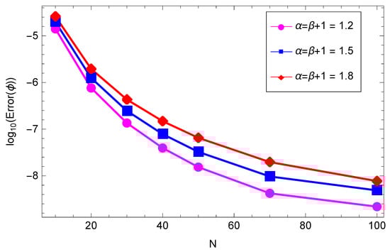
Figure 1.
Convergence order of in space for different values of and at .
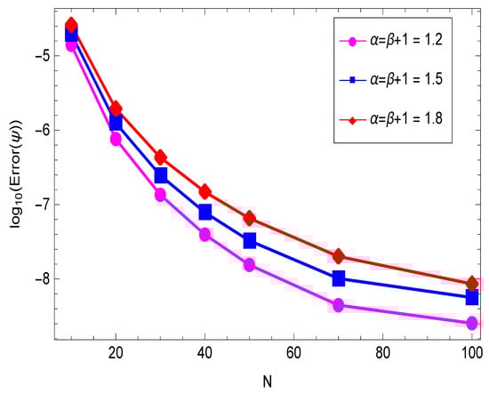
Figure 2.
Convergence order of in space for different values of and at .
Example 2 (Model output).
Consider the case of the coupled fractional Ginzburg–Landau Equations (1) with the initial values
and
Henceforth, we take
In this test, we select , and . Moreover, we will set the computational parameter and
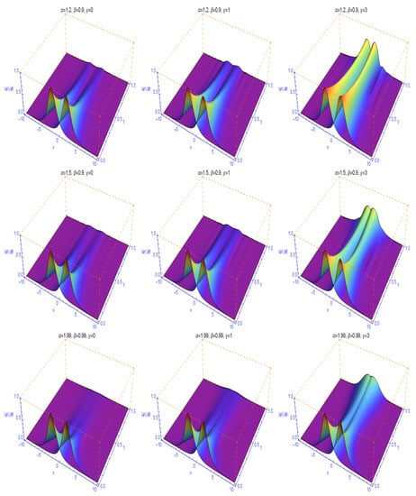
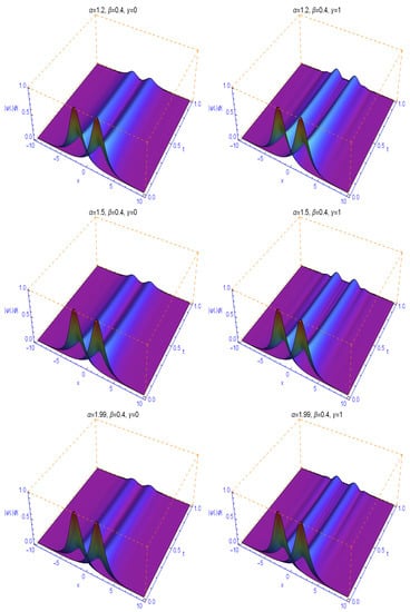
Figure 3 and Figure 4 display the numerical solutions for different α and β according to Example 2. We observe that, the fractional parameters α and β will dramatically affect the shape of the soliton, which is completely different from the classical case and shows the nonlocal character of the Caputo fractional derivative and fractional Laplacian. We find from these two figures also that the parameters and dramatically influence on the wave-shape. It is also observed that the numerical solutions decay fast with time evolution especially when the parameters and become more smaller and also when the fractional orders become more close to the integer orders, which means α comes close to 2 and β be closer to 1. These results seems to be in a good agreement with those appeared in ([33], Example 3).
Figure 3.
The evolution of and for different values of . The first row is presented at and . The second row is presented at and . The third row is done at and .
Figure 4.
The evolution of and for different values of . The first row is presented at and . The second row is presented at and . The third row is done at and .
6. Conclusions
In this work, we provided an efficient high order numerical scheme for the generalized fractional coupled Ginzburg–Landau system. This scheme has a second order of convergence with respect to time and spectral accuracy with respect to space. The convergence analysis of the scheme shows the unconditional convergence of its approximate solution. An algorithmic easy implementation of the scheme is also provided to facilitate its numerical application. The paper ends with a numerical example, it shows the agreement between the theoretical results and numerical ones. Finally, we need to clarify the following issues and present some future work:
- Our proposed high order hybrid numerical scheme is a linearized scheme of second order of convergence with respect to time inspite of the nonlinearity of the problem under consideration. The spectral accuracy is achieved due to the use of Galerkin Legendre approximation. Up to our knowledge, it is the first time that scheme is used to solve that kind of problems, especially noting the appearance of time and space fractional derivatives in the model under study. Unconditional convergence and stability of that scheme is secured, which means the error estimates of the numerical model has no dependence on time and spatial steps. This work reflects the possibility of that kind of schemes to be extended to deal with success with the singularity near the initial values of time fractional Caputo operators appearing in the generalized Ginzburg–Landau system. The latter can be secured by using nonuniform Alikhanov schemes combined with Legendre Galerkin spectral and it would be a near future plan for us.
- Due to the intrinsically nonlocal property and historical dependence of the fractional derivative, numerical applications of the numerical methods are always time-consuming. Therefore, fast schemes based on local approximations [41,42] can be implemented to avoid the high computational costs coming from the prehistory feature of spatial fractional order operators. Fast L1 and Fast Alikhanov formulas of the Caputo derivative which are based on the sum of exponentials can be used to to reduce the huge storage and computational cost [43,44]. Invoking these approaches to reduce the computational cost of finite difference/Galerkin spectral methods would be a target of our new works in the near future.
Author Contributions
All the authors contributed as follows. Conceptualization and methodology, M.A.Z., R.H.D.S. and A.S.H.; software and validation, R.H.D.S., A.S.H. and M.A.Z.; writing—original draft preparation, A.S.H., M.A.Z. and R.H.D.S.; writing—review and editing, M.A.Z., R.H.D.S. and A.S.H.; visualization, A.S.H., M.A.Z. and R.H.D.S.; funding acquisition and project administration, R.H.D.S., A.S.H. and M.A.Z. All authors have read and agreed to the published version of the manuscript.
Funding
The first author wishes to acknowledge the financial support of the National Research Centre of Egypt (NRC). The second author wishes to acknowledge the support of RFBR Grant 19-01-00019.
Data Availability Statement
Data sharing is not applicable to this article.
Acknowledgments
The authors wish to thank the reviewers for their comments and criticism. All of their comments were taken into account in the revised version of the paper, resulting in a substantial improvement with respect to the original submission.
Conflicts of Interest
The authors declare no conflict of interest.
References
- Ginzburg, V.L.; Landau, L.D. On the theory of superconductivity. In On Superconductivity and Superfluidity; Springer: Berlin/Heidelberg, Germany, 2009; pp. 113–137. [Google Scholar]
- Aranson, I.S.; Kramer, L. The world of the complex Ginzburg–Landau equation. Rev. Mod. Phys. 2002, 74, 99. [Google Scholar] [CrossRef]
- Tarasov, V.E.; Zaslavsky, G.M. Fractional Ginzburg–Landau equation for fractal media. Phys. A Stat. Mech. Its Appl. 2005, 354, 249–261. [Google Scholar] [CrossRef]
- Yang, L.; Huang, Q.W.; Dai, Z.D. Global attractor of nonlinear optical fibre materials with two cores. J. Hunan Univ. Nat. Sci. 2009, 3, 2621–2636. [Google Scholar]
- Sakaguchi, H.; Malomed, B.A. Stable solitons in coupled Ginzburg–Landau equations describing Bose–Einstein condensates and nonlinear optical waveguides and cavities. Phys. D Nonlinear Phenom. 2003, 183, 282–292. [Google Scholar] [CrossRef][Green Version]
- Pu, X.; Guo, B. Well-posedness and dynamics for the fractional Ginzburg–Landau equation. Appl. Anal. 2013, 92, 318–334. [Google Scholar] [CrossRef]
- Shen, T.; Huang, J. Well-posedness and dynamics of stochastic fractional model for nonlinear optical fiber materials. Nonlinear Anal. Theory Methods Appl. 2014, 110, 33–46. [Google Scholar] [CrossRef]
- Shen, J.; Tang, T.; Wang, L.L. Spectral Methods: Algorithms, Analysis and Applications; Springer: Berlin/Heidelberg, Germany, 2011. [Google Scholar]
- Zeng, F.; Liu, F.; Li, C.; Burrage, K.; Turner, I.; Anh, V. A Crank–Nicolson ADI spectral method for a two-dimensional Riesz space fractional nonlinear reaction-diffusion equation. SIAM J. Numer. Anal. 2014, 52, 2599–2622. [Google Scholar] [CrossRef]
- Zhang, H.; Jiang, X.; Wang, C.; Fan, W. Galerkin-Legendre spectral schemes for nonlinear space fractional Schrödinger equation. Numer. Algorithms 2018, 79, 337–356. [Google Scholar] [CrossRef]
- Guo, S.; Mei, L.; Zhang, Z.; Chen, J.; He, Y.; Li, Y. Finite difference/Hermite–Galerkin spectral method for multi-dimensional time-fractional nonlinear reaction–diffusion equation in unbounded domains. Appl. Math. Model. 2019, 70, 246–263. [Google Scholar] [CrossRef]
- Liu, H.; Lü, S. Galerkin spectral method for nonlinear time fractional Cable equation with smooth and nonsmooth solutions. Appl. Math. Comput. 2019, 350, 32–47. [Google Scholar] [CrossRef]
- Guo, S.; Mei, L.; Zhang, Z.; Jiang, Y. Finite difference/spectral-Galerkin method for a two-dimensional distributed-order time–space fractional reaction–diffusion equation. Appl. Math. Lett. 2018, 85, 157–163. [Google Scholar] [CrossRef]
- Guo, S.; Mei, L.; Zhang, Z.; Li, C.; Li, M.; Wang, Y. A linearized finite difference/spectral-Galerkin scheme for three-dimensional distributed-order time–space fractional nonlinear reaction–diffusion-wave equation: Numerical simulations of Gordon-type solitons. Comput. Phys. Commun. 2020, 252, 107144. [Google Scholar] [CrossRef]
- Zaky, M.A.; Hendy, A.S.; Macías-Díaz, J.E. Semi-implicit Galerkin–Legendre spectral schemes for nonlinear time-space fractional diffusion–reaction equations with smooth and nonsmooth solutions. J. Sci. Comput. 2020, 82, 1–27. [Google Scholar] [CrossRef]
- Zaky, M.A.; Hendy, A.S. Convergence analysis of an L1-continuous Galerkin method for nonlinear time-space fractional Schrödinger equations. Int. J. Comput. Math. 2020, 1–20. [Google Scholar] [CrossRef]
- Hendy, A.S.; Zaky, M.A. Global consistency analysis of L1-Galerkin spectral schemes for coupled nonlinear space-time fractional Schrödinger equations. Appl. Numer. Math. 2020, 156, 276–302. [Google Scholar] [CrossRef]
- Liao, H.l.; McLean, W.; Zhang, J. A discrete grönwall inequality with applications to numerical schemes for subdiffusion problems. SIAM J. Numer. Anal. 2019, 57, 218–237. [Google Scholar] [CrossRef]
- Hendy, A.S.; Macías-Díaz, J.E. A novel discrete Gronwall inequality in the analysis of difference schemes for time-fractional multi-delayed diffusion equations. Commun. Nonlinear Sci. Numer. Simul. 2019, 73, 110–119. [Google Scholar] [CrossRef]
- Hendy, A.S.; Macías-Díaz, J.E. A Discrete Grönwall Inequality and Energy Estimates in the Analysis of a Discrete Model for a Nonlinear Time-Fractional Heat Equation. Mathematics 2020, 8, 1539. [Google Scholar] [CrossRef]
- Zaky, M.A.; Hendy, A.S.; Macías-Díaz, J.E. High-order finite difference/spectral-Galerkin approximations for the nonlinear time–space fractional Ginzburg–Landau equation. Numer. Methods Partial Differ. Eq. 2020, 1–26. [Google Scholar] [CrossRef]
- Hendy, A.S.; Zaky, M.A. Graded mesh discretization for coupled system of nonlinear multi-term time-space fractional diffusion equations. Eng. Comput. 2020, 1–13. [Google Scholar] [CrossRef]
- Podlubny, I. Fractional Differential Equations. An Introduction to Fractional Derivatives, Fractional Differential Equations, Some Methods of Their Solution and Some of Their Applications; Academic Press: New York, NY, USA, 1999. [Google Scholar]
- Burrage, K.; Burrage, P.; Turner, I.; Zeng, F. On the analysis of mixed-index time fractional differential equation systems. Axioms 2018, 7, 25. [Google Scholar] [CrossRef]
- Abbaszadeh, M.; Dehghan, M. Numerical investigation of reproducing kernel particle Galerkin method for solving fractional modified distributed-order anomalous sub-diffusion equation with error estimation. Appl. Math. Comput. 2021, 392, 125718. [Google Scholar] [CrossRef]
- Abdullah, F.; Liu, F.; Burrage, P.; Burrage, K.; Li, T. Novel analytical and numerical techniques for fractional temporal SEIR measles model. Numer. Algorithms 2018, 79, 19–40. [Google Scholar] [CrossRef]
- Loghman, E.; Kamali, A.; Bakhtiari-Nejad, F.; Abbaszadeh, M. Nonlinear free and forced Vibrations of fractional modeled viscoelastic FGM micro-beam. Appl. Math. Model. 2021, 92, 297–314. [Google Scholar] [CrossRef]
- Abbaszadeh, M.; Dehghan, M. A POD-based reduced-order Crank-Nicolson/fourth-order alternating direction implicit (ADI) finite difference scheme for solving the two-dimensional distributed-order Riesz space-fractional diffusion equation. Appl. Numer. Math. 2020, 158, 271–291. [Google Scholar] [CrossRef]
- Zaky, M.A.; Hendy, A.S. An efficient dissipation–preserving Legendre–Galerkin spectral method for the Higgs boson equation in the de Sitter spacetime universe. Appl. Numer. Math. 2021, 160, 281–295. [Google Scholar] [CrossRef]
- Zaky, M.A.; Hendy, A.S.; Alikhanov, A.A.; Pimenov, V. Numerical analysis of multiterm fractional nonlinear subdiffusion equations with time delay: What could possibly go wrong? Commun. Nonlinear Sci. Numer. Simul. 2021, 96, 105672. [Google Scholar] [CrossRef]
- Abbaszadeh, M.; Dehghan, M. Direct meshless local Petrov–Galerkin (DMLPG) method for time-fractional fourth-order reaction–diffusion problem on complex domains. Comput. Math. Appl. 2020, 79, 876–888. [Google Scholar] [CrossRef]
- Xu, Y.; Zeng, J.; Hu, S. A fourth-order linearized difference scheme for the coupled space fractional Ginzburg–Landau equation. Adv. Differ. Equ. 2019, 2019, 455. [Google Scholar] [CrossRef]
- Li, M.; Huang, C. An efficient difference scheme for the coupled nonlinear fractional Ginzburg–Landau equations with the fractional Laplacian. Numer. Methods Partial Differ. Equ. 2019, 35, 394–421. [Google Scholar] [CrossRef]
- Pan, K.; Jin, X.; He, D. Pointwise error estimates of a linearized difference scheme for strongly coupled fractional Ginzburg–Landau equations. Math. Methods Appl. Sci. 2020, 43, 512–535. [Google Scholar] [CrossRef]
- Alikhanov, A.A. A new difference scheme for the time fractional diffusion equation. J. Comput. Phys. 2015, 280, 424–438. [Google Scholar] [CrossRef]
- Ervin, V.J.; Roop, J.P. Variational solution of fractional advection dispersion equations on bounded domains in Rd. Numer. Methods Partial Differ. Equ. 2007, 23, 256–281. [Google Scholar] [CrossRef]
- Wang, Y.; Liu, F.; Mei, L.; Anh, V.V. A novel alternating-direction implicit spectral Galerkin method for a multi-term time-space fractional diffusion equation in three dimensions. Numer. Algorithms 2020. [Google Scholar] [CrossRef]
- Shen, J. Efficient spectral-Galerkin method I. Direct solvers of second-and fourth-order equations using Legendre polynomials. SIAM J. Sci. Comput. 1994, 15, 1489–1505. [Google Scholar] [CrossRef]
- Cheng, B.; Guo, Z.; Wang, D. Dissipativity of semilinear time fractional subdiffusion equations and numerical approximations. Appl. Math. Lett. 2018, 86, 276–283. [Google Scholar] [CrossRef]
- Li, M.; Huang, C.; Wang, N. Galerkin finite element method for the nonlinear fractional Ginzburg–Landau equation. Appl. Numer. Math. 2017, 118, 131–149. [Google Scholar] [CrossRef]
- Zeng, F.; Turner, I.; Burrage, K. A stable fast time-stepping method for fractional integral and derivative operators. J. Sci. Comput. 2018, 77, 283–307. [Google Scholar] [CrossRef]
- Guo, L.; Zeng, F.; Turner, I.; Burrage, K.; Karniadakis, G.E. Efficient multistep methods for tempered fractional calculus: Algorithms and simulations. SIAM J. Sci. Comput. 2019, 41, A2510–A2535. [Google Scholar] [CrossRef]
- Liao, H.l.; Yan, Y.; Zhang, J. Unconditional convergence of a fast two-level linearized algorithm for semilinear subdiffusion equations. J. Sci. Comput. 2019, 80, 1–25. [Google Scholar] [CrossRef]
- Li, X.; Liao, H.l.; Zhang, L. A second-order fast compact scheme with unequal time-steps for subdiffusion problems. Numer. Algorithms 2020, 1–29. [Google Scholar] [CrossRef]
Publisher’s Note: MDPI stays neutral with regard to jurisdictional claims in published maps and institutional affiliations. |
© 2021 by the authors. Licensee MDPI, Basel, Switzerland. This article is an open access article distributed under the terms and conditions of the Creative Commons Attribution (CC BY) license (http://creativecommons.org/licenses/by/4.0/).