Experiments with Fuzzy Methods for Forecasting Time Series as Alternatives to Classical Methods

Abstract

Even though forecasting methods have advanced in the last few decades, economists still face a simple question: which prediction method gives the most accurate results? Econometric forecasting methods can deal with different types of time series and have good results, but in specific cases, they may fail to provide accurate predictions. Recently, new techniques borrowed from the soft computing area were adopted for economic forecasting. Starting from the importance of economic forecasts, we present an experimental study where we compared the accuracy of some of the most used econometric forecasting methods, namely the simple exponential smoothing, Holt and ARIMA methods, with that of two new methods based on the concept of fuzzy time series. We used a set of time series extracted from the Eurostat database and the R software for all data processing. The results of the experiments show that despite not being fully superior to the econometric techniques, the fuzzy time series forecasting methods could be considered as an alternative for specific time series.

1. Introduction

In terms of production and exchange relations, economic forecasts at a certain historical level have existed for many centuries. Scottish scientist and genius Adam Smith was among the first to take them seriously at the level of economics as a science. He defined the main economic categories, subjects and relationships in the form that we basically use them today. This concerns economic forecasts, economic models and their use and interpretation [1].

However, the need for economic forecasting was strongly shown by the great economic crisis of the 1930s, which again accelerated research in this area and reached a level that is still valid nowadays. After this catastrophe, economists, politicians and academic scientists focused on gaining an understanding of the real functioning of the economy and where the economy is heading. All this has led to the emergence, development and use of a wider range of statistical and analytical techniques, which have resulted in economic forecasts.

The principle of economic forecasting consists of a qualified effort to predict the future state of the economy using appropriately selected and reliably reported economic variables. They are one of the starting points for government decisions on investment, hiring, spending and other important policies that affect aggregate economic activity [2]. A correct estimate of future economic developments is essential for politicians and government officials, as it helps them to determine how to set the basic fiscal and monetary bases and instruments. Economists working in public administration play a crucial role in policy-making and in setting expenditure and tax parameters. In the area of fiscal policy, these are most often economic forecasts in relation to the amount of tax allocation depending on the forecasted GDP growth and public expenditure. Economic forecasting is important for the creation of plans and budgets in the medium and long term. In contrast, in the area of monetary policy, the main goal of central banks is to maintain a high degree of price stability, and this is primarily influenced by the development of demand and costs. Coyle [3] empirically compared the accuracy of model predictions with equilibrium correction mechanisms and models in differences (or growth rates) in a central bank inflation-targeting environment. As he noted, inflation forecasts for one or two years ahead are the primary source of information for monetary policy decisions in countries that use the inflation-targeting regime.

Thus, economic forecasts involve the creation of statistical models with the input of selected crucial variables, usually in an effort to focus on the future values for predicted economic indicators. These predicted economic indicators often include the inflation rate, interest rates, and the exchange rate as indicators for monetary policy, as well as industrial production, consumer confidence, labor productivity, retail sales and unemployment rate for the areas of fiscal and business policy.

The challenges and subjective aspects of people’s behavior in economic forecasts do not only affect the public sector. The private sector, commercial banks, investors, economists, academics, and also central banks have all issued economic forecasts that were partially or even wildly out of touch with reality [4].

Time series models that use historical economic data are popular methods of economic forecasting, while practice has verified that they are meaningful and competitive, mainly due to econometric systems of equations, especially in their multivariate forms.

Economic forecasting and prediction are often mentioned as ambiguous sciences. Due to the limited sources of data and their credibility, as well as the variously chosen methods, economic forecasting has its limits, which must be considered in practice and in scientific work [5]. Looking back, this is evident, for example, in assessing the reliability of crisis forecasting. The inability to record immediate declines reflects pressure on economists and forecasters to predict it sharply. Many of them prefer not to deviate from the mainstream because they keep in mind that bold projections could damage their reputation and the model’s future application [6].

Managers, business owners, investors and others should also not neglect the subjective nature of results and outputs within economic forecasts. Forecasts are strongly affected by the type of economic theory that forecasters use. Projections can vary very widely. One economist can believe in monetary policy, meaning that GDP growth is primarily influenced by the supply of money, and a second can argue that huge or even deficit spending is harmful for the economy. Thus, some of the outputs and conclusions do not come from qualified and credible economic analysis. On the contrary, they are usually determined on the basis of personal motives and assumptions about the functioning of markets and market forces. This inevitably means that the results of particular policies will be assessed differently [7].

The limits of the accuracy of economic forecasts also follow from the adoption of a certain economic theory as a basis for drawing conclusions. Economic theory can determine the background and basic features of a forecast, and economic knowledge and education can often play a key role. The educated economist should consider that certain conditions of time and place are specific and that the forecast provided by selected statistical methods may be adjusted while taking into account specific important circumstances. This is particularly important if a fundamentally uneconomic event also has significant economic consequences. If possible, the exact conclusion is not based purely on economic values; it is also necessary to consider uneconomic factors, including their future development. Predictions-based forecasts made only on the basis of subjective judgments cannot meet the strict requirements for the accuracy of outputs obtained by using objective techniques. As a result, the most reliable and the most trustworthy predictions are mostly based on fundamental and upgraded economic knowledge and standard statistical techniques.

The most frequent ant the most common form of errors in economic forecasting is probably still theoretical. Additionally, knowledge about the functioning of economic entities is relatively limited. Effective and accurate forecasting is also spoiled by the fact that economic conditions, economic policies and institutions change over time.

Time series represent consecutive series of observations measured at equal time intervals, and they are one of the most important concepts used to analyze economic processes and to make forecasts.

While the classical theory of econometric time series is well understood now [8,9], new techniques coming from the soft computing area have more recently been adopted for economic forecasts. The use of fuzzy sets in the area of analyzing and predicting time series came up based on the ability of fuzzy models to approximate functions and on the ease to understand the rules using linguistic variables by non-experts. Fuzzy time series methods have the advantage that they can deal with uncertainty or imprecision [10,11,12,13,14], which can be the case even for economic indicators computed based on data collected through probabilistic samples, or estimated using statistical models when the data are not available, or periodically updated based on the availability of new data sources (the revision policy for the datasets used in our experiments are given by the European Statistics Code of Practice, adopted by the European Statistical System Committee in 2011, and the European Statistical System Guidelines on the revision policy of the Principal European Economic Indicators), thus incorporating a certain degree of uncertainty.

Fuzzy time series were introduced by Song and Chisson [10], who developed the fuzzy time series model and applied it to some enrollment data series of University of Alabama, and later developed by Chen [11], who simplified the fuzzy time series prediction method using only arithmetic operations instead of max-min composition operations. Chen [12] also proposed a forecasting method based on high-order fuzzy time series of various orders: second, third, fourth and fifth. His experiments showed that the forecasts generated using the third-order model had better accuracy than other existing models.

Singh [13,15] proposed a new and computationally simplified method of fuzzy time series forecasting based on difference parameters. He tested his method on the same data series regarding students’ enrollment at the University of Alabama and compared the forecasted values obtained with his method against the results obtained by other existing methods to argue in favor of his method. Singh introduced a difference parameter as the fuzzy relation for forecasting and developed a forecasting algorithm of linear complexity.

Huarng [16] proposed a new heuristic model for time series forecasting using heuristic increasing and decreasing relations in order to increase the forecast accuracy. He tested his method on the same enrollments data and on Taiwan Future Exchange data.

Chen and Hsu [17] designed a first-order and time-variant forecast method starting form a division of the universe of discourse into intervals, and in a later stage re-dividing them into four, three, two and one depending on the statistical distribution of the data in each interval. The linguistic values represented by fuzzy sets are defined based on the intervals divided in the second stage, and then the data are fuzzified and the logical relationships are established. Finally, Chen’s method uses a set of rules to determine whether the forecasted data have an increasing or decreasing trend.

Recently, Liu et al. [18] proposed an ultra-short-term prediction approach based on the Takagi–Sugeno (T–S) fuzzy model, which has the advantage of a great linearization ability, by describing complex nonlinear systems by a number of linear or nearly linear systems and applied this model for wind power and wind speed forecast. The authors compared the results of their method with the results of some machine learning algorithms, showing the superiority of their method in increasing the forecasting accuracy.

Compared with classical time series forecasting methods, specific features of fuzzy time series add certain advantages: they do not require long series, and they can work with both crisp and fuzzy values. An extended overview of the fuzzy time series forecasting models was presented in Bose and Mali [14].

In this paper, using a set of time series with economic indicators, we compared the accuracy of some well-known econometric forecasting methods with that of two new methods based on the concept of fuzzy time series.

The next sections of the paper are organized as follows. In Section 2, we describe the data that we used in our experiments, the methods and the software used. In Section 3, we discuss the results that we obtained, and in the last section, we present the main conclusions and directions for future work.

2. Data and Methods

We used data series from the Eurostat database to test all the methods used in this study. Thus, we selected 3 monthly economic indicators that we considered important to assess the economic activity of a country from the Eurostat database with values from January 2017 to February 2020:

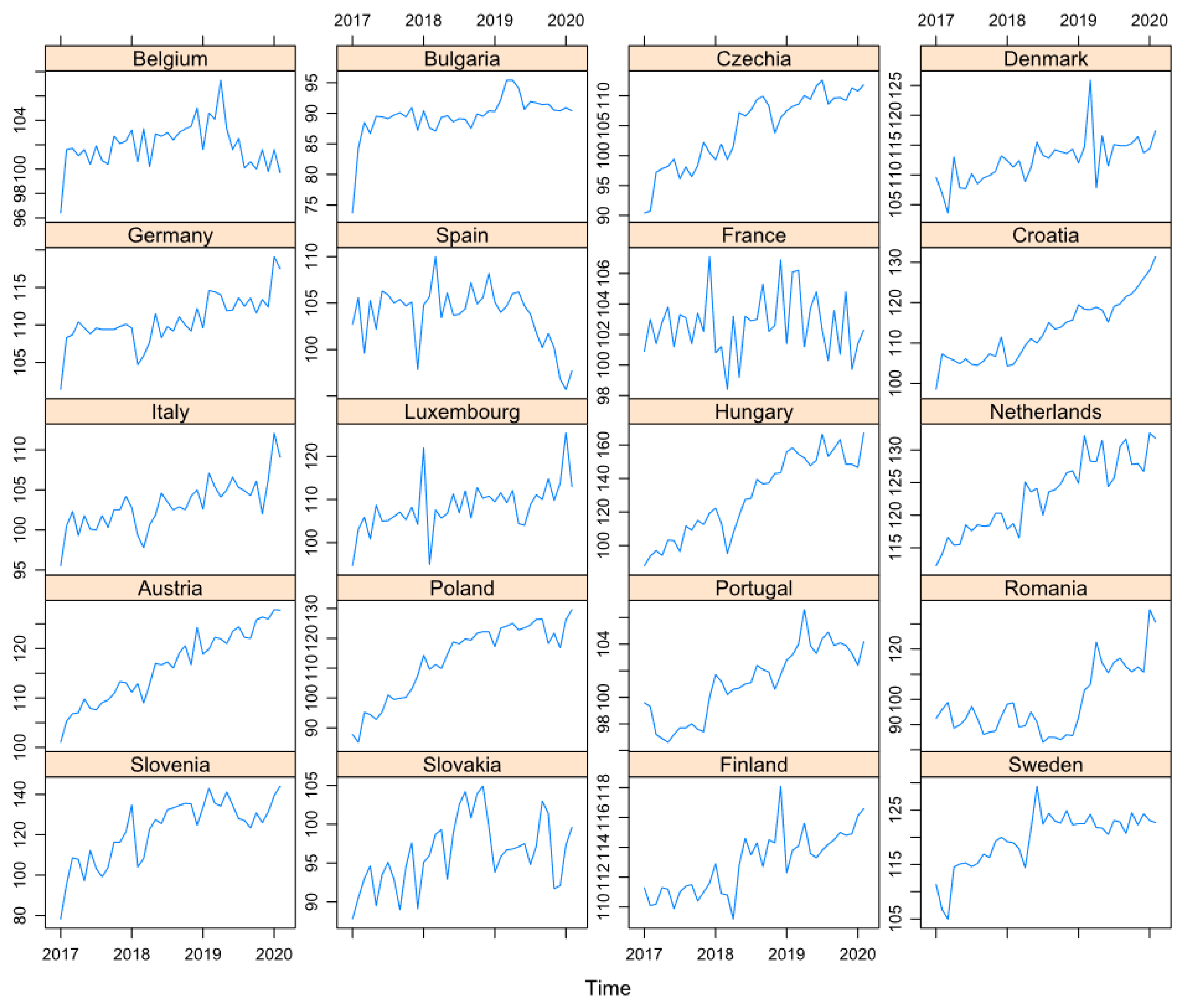
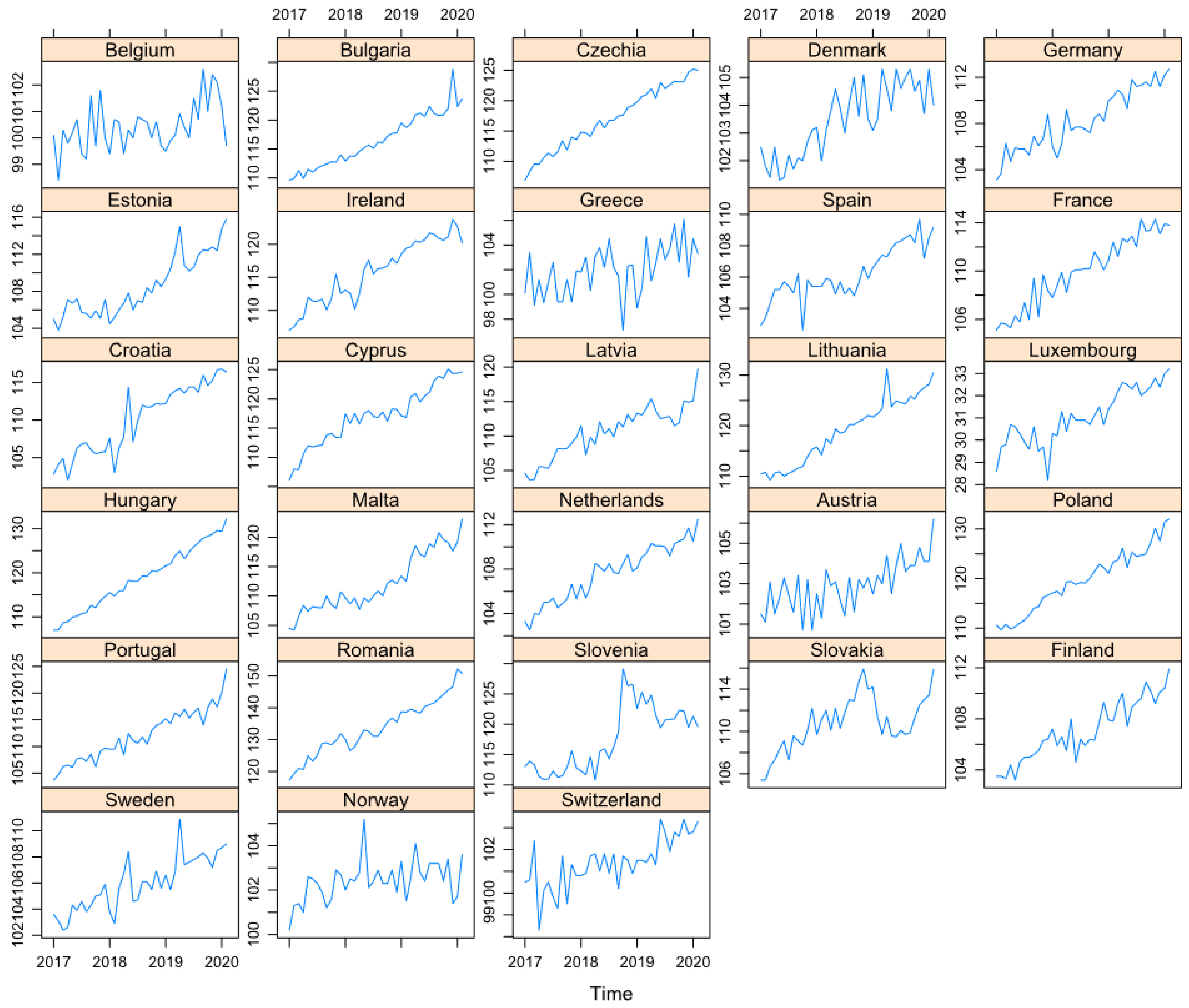
• The volume index of production in construction (2015 = 100), seasonally and calendar-adjusted, for 20 European countries;
• The volume index of production in the industry for electricity, gas, steam and air conditioning supply (2015 = 100), seasonally and calendar-adjusted, for 29 European countries;
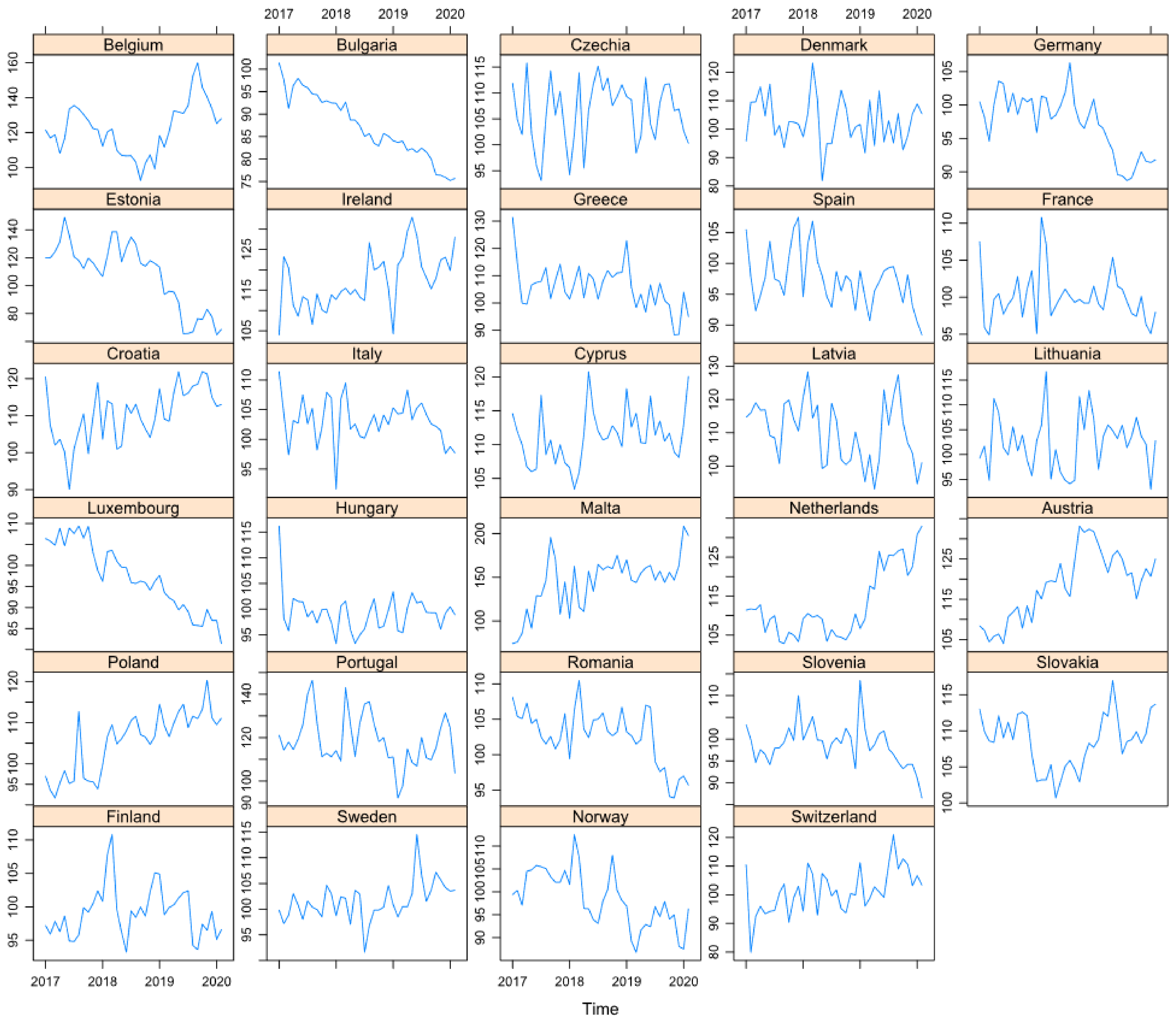
• The index of deflated turnover in retail trade, except for motor vehicles and motorcycles (2015 = 100), seasonally and calendar-adjusted, for 28 European countries.

From the available data series in the Eurostat database, we eliminated those countries with missing values for the time series, because we did not want the results to be influenced by an external factor such as the imputation method. The econometric methods used in our analysis are sensitive to missing values. In Figure 1, Figure 2 and Figure 3, we show a graphical representation of the datasets, while in

Table 1. Descriptive statistics for the volume index of production in construction.

Country	Min	1sq QU	Median	Mean	3rd QU	Max	VAR	SD	SE	Order of Integration
Belgium	96.4	100.62	101.8	101.95	103	107.3	3.41	1.84	0.29	1
Bulgaria	73.7	89.02	89.8	89.55	90.82	95.4	11.68	3.41	0.55	1
Czechia	90.4	99.3	106.9	104.35	109.4	112.6	37.59	6.13	0.99	1
Denmark	103.6	109.97	112.9	112.49	114.62	125.9	14.47	3.8	0.61	1
Germany	101.4	109.25	109.9	110.63	112.35	119.1	10.38	3.22	0.52	1
Spain	95.7	102.32	104.7	103.73	105.6	110	9.84	3.13	0.5	1
France	98.4	101.25	102.7	102.65	103.55	107.1	4.1	2.02	0.32	2
Croatia	98.5	106.47	112.75	113.19	118.77	131.4	59.73	7.72	1.25	1
Italy	95.5	101.8	102.7	103.13	104.97	112.1	9.59	3.09	0.5	0
Luxembourg	94.6	105.4	108.45	108.38	111.25	125.4	33.24	5.76	0.93	0
Hungary	87.8	109.82	132.5	129.62	150.3	167.1	584.79	24.18	3.92	1
Netherlands	112.2	118.42	124	123.18	127.55	132.6	32.42	5.69	0.92	1
Austria	101	110.07	116.85	116.45	122.25	127.9	51.63	7.18	1.16	1
Poland	85.1	101.5	117.65	112.87	122.65	129.6	153.12	12.37	2	1
Portugal	96.6	99.37	101.45	101.19	103.3	106.6	7.12	2.66	0.43	0
Romania	82.9	88.7	94.1	99.12	110.82	135.7	187.49	13.69	2.22	2
Slovenia	78.3	109.5	126.55	122.38	134.42	144.1	240.89	15.52	2.51	1
Slovakia	87.8	93.12	96.35	96.28	99.2	104.9	19.69	4.43	0.71	2
Finland	109.2	111.22	113.1	112.95	114.45	118.1	4.37	2.09	0.33	1
Sweden	105	116.45	121.6	119.68	122.77	129.4	25.35	5.03	0.81	1

,

Table 2. Descriptive statistics for the volume index of production in industry for electricity, gas, steam and air conditioning supply.

Country	Min	1sq QU	Median	Mean	3rd QU	Max	VAR	SD	SE	Order of Integration
Belgium	92.6	110.35	121.65	122.2	132.4	159.9	219.59	14.81	2.4	2
Bulgaria	75.2	82.32	85.7	87.2	92.67	101.4	50.36	7.09	1.15	2
Czechia	93.1	102.02	106.8	106.27	111.6	115.8	37.19	6.09	0.98	1
Denmark	81.9	96.12	102.55	102.68	108.6	123.3	67.67	8.22	1.33	0
Germany	88.7	93.55	98.35	97.24	100.8	106.3	20.83	4.56	0.74	1
Estonia	64.7	89.55	115.95	107.56	121.15	149	573.3	23.94	3.88	2
Ireland	104	112.85	115.5	117.23	121.87	132.9	47.79	6.91	1.12	0
Greece	88.3	101.02	106.65	105.8	110.45	131.4	67.52	8.21	1.33	1
Spain	88.4	94.6	97.35	97.43	99.17	107.5	20.54	4.53	0.73	1
France	94.9	97.85	99.55	100.01	101.1	110.8	11.68	3.41	0.55	1
Croatia	90.1	104.52	110.55	110.34	115.92	121.9	54.83	7.4	1.2	1
Italy	91.6	101.55	102.95	103.11	105.27	111.4	14.4	3.79	0.61	1
Cyprus	103.4	108.6	110.85	111.25	112.95	120.8	15.9	3.98	0.64	0
Latvia	93	101.9	111.4	110.37	117.95	128.4	86.67	9.3	1.51	1
Lithuania	93	98.97	102.8	102.48	105.82	116.7	31.44	5.6	0.9	0
Luxembourg	81.4	90.92	96.25	97.29	104.42	109.4	63.53	7.97	1.29	2
Hungary	93.3	96.4	99.35	99.26	101.05	116.2	14.79	3.84	0.62	1
Malta	74.2	128.52	150.7	144.28	162.67	208.7	1012.44	31.81	5.16	1
Netherlands	102.8	105.72	110	112.86	119.62	133	77.63	8.81	1.42	2
Austria	104	112.15	119.45	118.47	124.87	133.2	69.5	8.33	1.35	2
Poland	91.7	97.32	106.9	105.45	111.07	120.3	54.89	7.4	1.2	1
Portugal	92.2	111.12	116.55	118.68	126.2	146.4	141.07	11.87	1.92	1
Romania	93.9	100.97	102.95	102.62	105.32	110.5	15.58	3.94	0.64	1
Slovenia	86.5	95.75	99	98.77	101.02	113.5	23.83	4.88	0.79	1
Slovakia	100.7	106	108.7	108.56	112.07	117	14.02	3.74	0.6	2
Finland	93.2	96.35	99	99.15	100.72	110.8	14.51	3.8	0.61	1
Sweden	91.6	99.8	101.2	101.56	103.65	114.5	14.08	3.75	0.6	1
Norway	86.8	94.15	97.95	98.44	103	112.5	37.45	6.12	0.99	0
Switzerland	79.9	95.32	100.8	101.37	107.07	121	61.67	7.85	1.27	1

and

Table 3. Descriptive statistics for the index of deflated turnover in retail trade, except for motor vehicles and motorcycles.

Country	Min	1sq QU	Median	Mean	3rd QU	Max	VAR	SD	SE	Order of Integration
Belgium	98.4	99.82	100.3	100.42	100.77	102.6	0.82	0.9	0.14	1
Bulgaria	109.6	112.72	115.9	116.5	120.75	128.8	21.38	4.62	0.75	2
Czechia	106.9	113.45	116.8	116.99	121.75	125.2	26.74	5.17	0.83	1
Denmark	101.3	102.5	103.55	103.48	104.6	105.3	1.59	1.26	0.2	1
Germany	103.1	106.15	107.95	108.29	110.8	112.7	6.91	2.62	0.42	1
Estonia	103.8	105.92	107.5	108.53	110.75	115.8	10.58	3.25	0.52	1
Ireland	107	111.85	116.35	115.83	120.27	123.8	22.26	4.71	0.76	0
Greece	97.1	100.62	102.2	101.96	103.25	106.1	4.12	2.03	0.32	1
Spain	102.6	105.22	105.8	106.21	107.37	109.7	2.87	1.69	0.27	1
France	105.1	107.9	110.1	109.98	112.4	114.3	8.12	2.85	0.46	1
Croatia	102	106.07	111.75	110.06	114.12	116.8	20.76	4.55	0.73	1
Cyprus	106.1	113.5	117.25	117.01	120.45	125.1	24.28	4.92	0.79	1
Latvia	103.6	108.2	111.4	110.61	112.95	119.7	13.3	3.64	0.59	1
Lithuania	109.2	112.4	119.8	118.98	124.15	131.2	41.51	6.44	1.04	1
Luxembourg	28.2	30.3	30.9	31.06	32.2	33.2	1.52	1.23	0.2	1
Hungary	107	112.87	118.75	118.75	124.5	132.2	50.62	7.11	1.15	1
Malta	104.2	108.42	110.35	112.26	117	123.1	24.77	4.97	0.8	1
Netherlands	102.5	105.32	107.95	107.64	109.85	112.5	6.46	2.54	0.41	1
Austria	100.7	102.22	103.1	102.93	103.67	106.2	1.51	1.23	0.19	1
Poland	109.6	114.77	119.35	119.6	124.3	132	39.71	6.3	1.02	1
Portugal	103.7	108.45	111.7	112.09	115.52	124.5	22.65	4.75	0.77	2
Romania	117.3	128.5	132.85	133.76	139.45	152.2	73.99	8.6	1.39	1
Slovenia	110.8	112.82	116.15	117.53	121.45	129.1	28.21	5.31	0.86	2
Slovakia	105.4	109.52	110.2	110.75	112.42	115.9	6.67	2.58	0.41	3
Finland	103.2	105.27	106.5	107.06	109.2	111.9	5.53	2.35	0.38	2
Sweden	102.4	104.37	105.75	105.93	107.55	110.9	4.13	2.03	0.32	0
Norway	100.2	101.9	102.4	102.42	102.9	105.2	0.84	0.91	0.14	0
Switzerland	98.3	100.8	101.5	101.39	101.87	103.4	1.35	1.16	0.18	1

, we present descriptive statistics and the order of integration for each economic indicator selected and each country. We checked all the time series for seasonality using the Webel–Ollech overall seasonality test (WO test) [19], and none have a seasonal component, as we expected.

To test whether fuzzy time series models can be used as an alternative for time series forecasting and based on an overview study [20] that indicates exponential smoothing, moving average and autoregressive methods as the most widely used econometric forecasting techniques, we used the simple exponential smoothing, Holt and the ARIMA methods, and then compared the accuracy of predictions with the results obtained by using fuzzy methods.

The exponential smoothing method has been developed and used for time series forecasting since the 1950s [21,22], but only recently some procedures for automatic model selection were designed [23,24]. Exponential smoothing is a set of methods that was classified initially by Pegels [25], and then by Gardner [26], and Taylor [27]. In our study, we used the simple exponential smoothing method (sometimes called single exponential smoothing) [20] and the Holt method [28].

The simple exponential smoothing method (SEM) is usually applied for forecasting data, which do not exhibit a clear trend or seasonal pattern. For y_t time series, the one-step-ahead forecast for time t + 1 through the SEM method is:

$${\widehat{\mathrm{y}}}_{\mathrm{t}+1|\mathrm{t}}={\mathsf{\alpha }\mathrm{y}}_{\mathrm{t}}+\left(1-\mathsf{\alpha }\right){\widehat{\mathrm{y}}}_{\mathrm{t}|\mathrm{t}-1})$$

(1)

which means that one time ahead prediction is a weighted average between the most recent observation and the previous predicted value. We can write:

$${\widehat{\mathrm{y}}}_{\mathrm{t}+1|\mathrm{t}}={\widehat{\mathrm{y}}}_{\mathrm{t}|\mathrm{t}-1}+\mathsf{\alpha }\left({\mathrm{y}}_{\mathrm{t}}-{\widehat{\mathrm{y}}}_{\mathrm{t}|\mathrm{t}-1}\right)$$

(2)

or

$${\widehat{\mathrm{y}}}_{\mathrm{t}+1|\mathrm{t}}={\widehat{\mathrm{y}}}_{\mathrm{t}|\mathrm{t}-1}+{\mathsf{\alpha }\mathrm{e}}_{\mathrm{t}}$$

(3)

where ${\widehat{\mathrm{y}}}_{\mathrm{t}+1|\mathrm{t}}$ is the smoothed value of the data series carried out at time t for t + 1, ${\widehat{\mathrm{y}}}_{\mathrm{t}|\mathrm{t}-1}$ is the previous forecast, ${\mathrm{e}}_{\mathrm{t}}={\mathrm{y}}_{\mathrm{t}}-{\widehat{\mathrm{y}}}_{\mathrm{t}|\mathrm{t}-1}$ is the forecasting error at time t, and 0 ≤ α ≤ 1 is the smoothing parameter. That is, the series forecasted value for time t + 1 is calculated as the forecasted value for time t, corrected with a proportion (α) of the forecast error. The smoothing parameter α is either exogenous or is calculated to minimize the in-sample sum of squared errors.

The simple exponential smoothing is generally appropriate for series that are random walk with or without drift. The Holt exponential smoothing method is a better forecasting method for data that reveal a linear trend, as it can be described as follows:

$$\mathrm{Forecast} \mathrm{equation}: {\widehat{\mathrm{y}}}_{\mathrm{t}+\mathrm{h}|\mathrm{t}}={ \mathrm{L}}_{\mathrm{t}}+{ \mathrm{hb}}_{\mathrm{t}}$$

(4)

$$\mathrm{Level} \mathrm{equation}: {\mathrm{L}}_{\mathrm{t}}={ \mathsf{\alpha }\mathrm{y}}_{\mathrm{t}}+\left(1- \mathsf{\alpha }\right)\left({\mathrm{L}}_{\mathrm{t}-1}+{ \mathrm{b}}_{\mathrm{t}-1}\right)$$

(5)

$$\mathrm{Trend} \mathrm{equation}: {\mathrm{b}}_{\mathrm{t}}= \mathsf{\beta }\left({\mathrm{L}}_{\mathrm{t}}-{ \mathrm{L}}_{\mathrm{t}-1}\right)+\left(1- \mathsf{\beta }\right){\mathrm{b}}_{\mathrm{t}-1}$$

(6)

where ${\widehat{\mathrm{y}}}_{\mathrm{t}+\mathrm{h}|\mathrm{t}}$ is the forecast carried out at time $\mathrm{t}$ for period t + h (h = 1, 2, …), L_t and ${\mathrm{L}}_{\mathrm{t}-1}$ are the smoothed values of the level at time t and t − 1, respectively, b_t and ${\mathrm{b}}_{\mathrm{t}-1}$ denote the smoothed values for the trend, and 0 ≤ α ≤ 1 and 0 ≤ β ≤ 1 are the smoothing parameters for the level (α) and the trend (β), respectively. The smoothing parameters are exogenous, or they are calculated by using the sum of squared errors criterion (SSE) (or, alternatively the mean squared error (MSE), and root mean square errors (RMSE)).

Auto Regressive Integrated Moving Average (ARIMA) models [29,30] are widely used methods in the analysis and prediction of time series. In addition to exponential smoothing methods, ARIMA models aim to identify the stationarity and the autocorrelations in the data. The models are usually denoted as ARIMA(p, d, q), using p as the order (number of time lags) of the autoregressive part of the model, d to denote the degree of differencing and q for the order of the moving-average part. For a times series y_t (possibly non-stationary in the sense of mean, but not non-stationary in variance/autocovariance), the ARIMA(p, d, q) model can be written as:

$$\left(1-{\mathsf{\varphi }}_1\mathrm{L} -{\mathsf{\varphi }}_2{\mathrm{L}}^2 -\dots - {\mathsf{\varphi }}_{\mathrm{p}}{\mathrm{L}}^{\mathrm{p}}\right){\left(1- \mathrm{L}\right)}^{\mathrm{d}}{\mathrm{y}}_{\mathrm{t}}=\left(1+{\mathsf{\theta }}_1\mathrm{L}+{\mathsf{\theta }}_2{\mathrm{L}}^2+\dots +{\mathsf{\theta }}_{\mathrm{q}}{\mathrm{L}}^{\mathrm{q}}\right){\mathsf{\epsilon }}_{\mathrm{t}}$$

(7)

where L is the lag (backshift) operator (so that ${\mathrm{Ly}}_{\mathrm{t}}={ \mathrm{y}}_{\mathrm{t}-1}$), ${\mathsf{\varphi }}_1, \dots , {\mathsf{\varphi }}_{\mathrm{p}}$ are the $\mathrm{p} \mathrm{coefficients}$ in the autoregressive part of the model, ${\mathsf{\theta }}_1, \dots , {\mathsf{\theta }}_{\mathrm{q}}$ are the q coefficients in the moving average part of the model, and ε_t is white noise. In polynomial notation, the ARIMA model can be written as:

$$\mathsf{\Phi }\left(\mathrm{L}\right){\left(1-\mathrm{L}\right)}^{\mathrm{d}}{\mathrm{y}}_{\mathrm{t}}=\mathsf{\Theta }\left(\mathrm{L}\right){\mathsf{\epsilon }}_{\mathrm{t}}$$

(8)

where Φ(L) is a polynomial function of order p (the autoregressive part of the model), Θ(L) is a polynomial function of order q (the moving average part), and d is the order of integration (degree of differencing involved). A detailed discussion about ARIMA models can be found in Hamilton [9].

Besides classical methods of time series analysis, new, unconventional approaches have been developed based on the theory of fuzzy sets [31]. Among some of the most well-known time series analysis and forecasting methods based on fuzzy set theory, we can mention the Song and Chissom [10], Chen [11,12], Singh [13,15], heuristic [16], Chen–Hsu [17], Abbasov–Mamedova [32], and NFTS [33] methods. The first five methods cited above are used to fit/forecast time series even when historical values change over time. This could occur when the values of the time series are updated or changed due to different reasons, for example when new data are available to compute them. The last two methods allow users to make predictions for various time horizons.

Below, we present a very short introduction to the fuzzy time series concept. For more details, an interested reader can find a comprehensive review of fuzzy time series forecasting models in Bose and Mali [14].

Assuming that:

$$\mathrm{U} =\left\{{\mathrm{u}}_1,{ \mathrm{u}}_2, \dots ,{ \mathrm{u}}_{\mathrm{n}}\right\}$$

(9)

is the universe of discourse where u_i, i = 1 … n are the linguistic values, we can define the fuzzy set of linguistic variables A_i of U as:

$${\mathrm{A}}_{\mathrm{i}}={ \mathsf{\mu }}_{{\mathrm{A}}_{\mathrm{i}}}\left({\mathrm{u}}_1\right)/{\mathrm{u}}_1+{ \mathsf{\mu }}_{{\mathrm{A}}_{\mathrm{i}}}\left({\mathrm{u}}_2\right)/{\mathrm{u}}_2+\dots +{\mathsf{\mu }}_{{\mathrm{A}}_{\mathrm{i}}}\left({\mathrm{u}}_{\mathrm{n}}\right)/{\mathrm{u}}_{\mathrm{n}}$$

(10)

where ${\mathsf{\mu }}_{{\mathrm{A}}_{\mathrm{i}}}$ is the membership function of the fuzzy set A_i, ${\mathsf{\mu }}_{{\mathrm{A}}_{\mathrm{i}}}: \mathrm{U}\to \left[0,1\right]$, and ${\mathsf{\mu }}_{{\mathrm{A}}_{\mathrm{i}}}\left({\mathrm{u}}_{\mathrm{j}}\right)$ represents the degree of belonging of ${\mathrm{u}}_{\mathrm{j}}$ to the fuzzy set A_i.

Let us assume that ${\mathrm{Z}}_{\mathrm{t}} \left(\mathrm{t} =0, 1, 2, \dots \right)$ is a subset of $ℝ$ and it is also the universe of discourse of the fuzzy sets ${\mathrm{y}}_{\mathrm{i}}\left(\mathrm{t}\right), \mathrm{i} =0, 1, 2, \dots$. If Y(t) is the collection of ${\mathrm{y}}_1\left(\mathrm{t}\right),{ \mathrm{y}}_2\left(\mathrm{t}\right)$,…, then Y(t) is a fuzzy time series defined over Z_t. If Y(t) is caused only by Y(t − 1), which we will denote by $\mathrm{Y}\left(\mathrm{t}-1\right)\to \mathrm{Y}\left(\mathrm{t}\right),$ then a fuzzy relationship is established between Y(t) and Y(t − 1), and it can be written as the following fuzzy relational equation:

$$\mathrm{Y}\left(\mathrm{t}\right)= \mathrm{Y}\left(\mathrm{t}-1\right)\circ \mathrm{R}\left(\mathrm{t}, \mathrm{t}-1\right)$$

(11)

where $\circ$ is the max-min composition operator and R is a relation named the first-order model of Y(t). If $\mathrm{R}\left(\mathrm{t}, \mathrm{t}-1\right)$ is independent of time, $\mathrm{R}\left({\mathrm{t}}_1,{ \mathrm{t}}_2-1\right)= \mathrm{R}\left({\mathrm{t}}_2,{ \mathrm{t}}_2-1\right)$ for ${\mathrm{t}}_1\ne {\mathrm{t}}_2$ then Y(t) is called time invariant fuzzy time series.

If Y(t) is determined by several fuzzy sets $\mathrm{Y}\left(\mathrm{t}-\mathrm{n}\right), \mathrm{Y}(\mathrm{t}-\mathrm{n}+1, \dots , \mathrm{Y}\left(\mathrm{t}-1\right)$, then the fuzzy relationship is denoted as: ${\mathrm{A}}_{\mathrm{i}1},{ \mathrm{A}}_{\mathrm{i}2}, \dots ,{ \mathrm{A}}_{\mathrm{in}}\to {\mathrm{A}}_{\mathrm{j}}$ where ${\mathrm{A}}_{\mathrm{i}1}=\mathrm{Y}\left(\mathrm{t}-\mathrm{n}\right), \dots ,{\mathrm{A}}_{\mathrm{in}}=\mathrm{Y}\left(\mathrm{t}-1\right)$. This is called nth-order fuzzy time series model.

In cases when Y(t) is simultaneously determined by $\mathrm{Y}\left(\mathrm{t}-1\right), \mathrm{Y}\left(\mathrm{t}-2\right), \dots , \mathrm{Y}\left(\mathrm{t}-\mathrm{k}\right), \mathrm{k}>0$ and the relations are time variant, then Y(t) is called the time variant fuzzy time series and we have:

$$\mathrm{Y}\left(\mathrm{t}\right)= \mathrm{Y}\left(\mathrm{t}-1\right)\circ {\mathrm{R}}^{\mathrm{w}}\left(\mathrm{t}, \mathrm{t}-1\right)$$

(12)

where w > 1 is a time parameter by which Y(t) is affected, and there are several methods to compute the relation ${\mathrm{R}}^{\mathrm{w}}\left(\mathrm{t}, \mathrm{t}-1\right)$ ranging from the max-min composition operations to more simplified rules.

The foundation of fuzzy time series forecasting was set by Song and Chissom [10] and later developed by various researchers. Thus, the Chen method [11] is basically an adapted version of the method presented in [10], but it is more efficient because it simplifies the arithmetic operations. Chen [11] provides a detailed description of the fitting procedure and showed that it can make robust predictions even in cases when the historical data are not accurate.

According to Chen, fuzzy time series analysis and forecasting consist of the following processing stages:

• Set the universe of discourse
• Divide the universe of discourse into several intervals
• Fuzzify the datasets
• Setting the fuzzy logical relationship and group
• Defuzzification.

Huarng [16] proposed heuristic forecasting models through the integration of problem-specific heuristic knowledge with Chen’s model to obtain predictions that are more accurate. The empirical studies conducted by the author showed that the heuristic approach better reflects the fluctuations in fuzzy time series and obtained better overall forecasting results compared with previously developed methods.

The Chen–Hsu forecasting method [17] belongs to the first order and time-variant class of methods, and improves Chen’s method, obtaining a better prediction accuracy measured with MSE.

Singh [13,15] developed a forecasting method based on fuzzy time series which can efficiently cope up with cases when there are large fluctuations in consecutive values of the time series. Singh tested the method on time series from crop production and compared its accuracy with other existing methods, showing the superiority of his approach. His method can be summarized as:

• Define U as the universe of discourse starting from the range of time series data, setting $\mathrm{U} =\left[{\mathrm{Y}}_{\min }-{ \mathrm{D}}_1,{ \mathrm{Y}}_{\max }-{ \mathrm{D}}_2\right]$, with D₁ and D₂ being two convenient positive numbers
• Divide U into equal length intervals u₁, u₂, … u_k. The number of intervals should be equal to the number of linguistic variables A₁, A₂, … A_k
• Build the fuzzy sets A_i according to the previously set intervals and apply triangular membership rule to each one
• Fuzzify the available data and set the fuzzy logical relations ${\mathrm{A}}_{\mathrm{i}}\to {\mathrm{A}}_{\mathrm{j}}$ where A_i corresponds to the fuzzified value at time step n and A_j to the time step n + 1.
• Define the rules for forecasting. An interested reader is invited to consult [8,13] for a detailed description of the rules.

For our forecasting experiments, we chose the Abbasov–Mamedova and NFTS methods because they easily allow us to make predictions for a future time horizon, and they have efficient implementations.

Starting from a population forecasting problem, Abbasov and Mamedova [32] proposed a new method of time series forecasting that can even use incomplete, fuzzy input data. They successfully applied their procedure to demographic data, showing the effectiveness of the proposal. Their proposal can be described as follows:

• Define the universe of discourse (U) starting from the range of time series data;
• Divide the set U into equal-length intervals
• Determine the respective values of linguistic variable
• Fuzzify the input data
• Select the parameter W > 1, and compute the fuzzy relationships matrix
• Defuzzify the obtained results.

In the first step, the universal set U is set as $\mathrm{U} =\left[{\mathrm{Y}}_{\min }-{ \mathrm{D}}_1,{ \mathrm{Y}}_{\max }-{ \mathrm{D}}_2\right]$, where D₁ and D₂ are two positive numbers, and then this set is divided into several equal intervals. The default number of intervals is 7, and the fuzzy set ${\mathrm{A}}_1,{ \mathrm{A}}_2, \dots ,{ \mathrm{A}}_7$ is defined on the universal set U by using the following equation: ${\mathsf{\mu }}_{{\mathrm{A}}_{\mathrm{i}}}=\frac{1}{1+{\left[\mathrm{C}·\left(\mathrm{U}-{\mathrm{u}}_{\mathrm{m}}^{\mathrm{i}}\right)\right]}^2}$, where ${\mathrm{u}}_{\mathrm{m}}^{\mathrm{i}}$ is the corresponding interval. After selecting a value for the w parameter, the ${\mathrm{R}}^{\mathrm{w}}$ relationship matrix is computed, and then the forecasted value can be calculated. For a detailed description of this method, an interested reader can consult [32].

The NFTS [33] method can interpolate historical data to make predictions. It normalizes the original data, and automatically computes the number of clusters and finds the fuzzy relationships of each element in series to the clusters. The convergence of the method is theoretically demonstrated and experimentally tested by the authors. The accuracy of predictions was compared with other existing models using several well-known datasets, showing the advantages of their proposal. The novelty of this method starts with the procedure of computing the number of clusters for the universal set U. While other methods set this number to a constant, the NTFS method proposes an automatic iterative algorithm to determine the optimal number of clusters (suitable number of clusters (SNC)). Then, to determine the elements in each cluster and also the fuzzy relation of each element to the cluster, one can use an automatic iterative procedure. The authors of this method demonstrated the convergence of the proposed iterative procedures for all times series.

We used already existing implementations of the above-mentioned forecasting methods, namely the AnalyzeTS R package [34] for the Abbasov–Mamedova and NFTS fuzzy methods.

We employed a standard technique and divided each times series used for experimentation in two parts: a first part used for model fitting (training) and a second part for testing and measuring out-of-sample prediction errors. The second part contains 2, 4 or 6 values for each time series and methods tested, thus measuring the performance of forecasting methods for 2, 4 and 6 steps ahead. The accuracy of forecasting models was evaluated using the mean absolute error (MAE), which reflects the amplitude of errors, the mean absolute percent error (MAPE), which is equivalent to standardized MAE and reflects absolute corresponding degree, the root of mean square error (RMSE), which reflects the closeness of the error distribution, and the mean absolute scaled error (MASE), a measure proposed in Hyndman and Koehler [35]. The formulas for computing these accuracy measures are given in Equations (13)–(16). We mention that MAPE is particularly important for time series with strong trends. MAE and RMSE are considered scale-dependent errors, MAPE is a percentage accuracy measure and is consequently unit free, and MASE is a scaled accuracy measure, considered a good alternative to percentage errors. MAE is very popular, being easy to understand and compute, and minimizing MAE will lead to forecasts of the median, while minimizing the value of the RMSE will lead to forecasts of the mean. The RMSE is also extensively used in forecasting applications, although it implies computations that are more complex.

$$\mathrm{MAE}\left({\mathrm{y}}_{\mathrm{pred}}, \mathrm{y}\right)=\frac{{{\displaystyle \sum }}_{\mathrm{t}=1}^{\mathrm{n}}\left|{\mathrm{y}}_{\mathrm{pred},\mathrm{t}}-{\mathrm{y}}_{\mathrm{t}}\right|}{\mathrm{n}}$$

(13)

$$\mathrm{MAPE}\left({\mathrm{y}}_{\mathrm{pred}}, \mathrm{y}\right)=\frac{{{\displaystyle \sum }}_{\mathrm{t}=1}^{\mathrm{n}}\frac{\left|{\mathrm{y}}_{\mathrm{pred},\mathrm{t}}-{\mathrm{y}}_{\mathrm{t}}\right|}{\left|{\mathrm{y}}_{\mathrm{t}}\right|}}{\mathrm{n}}$$

(14)

$$\mathrm{RMSE}\left({\mathrm{y}}_{\mathrm{pred}}, \mathrm{y}\right)=\sqrt{{\displaystyle \sum }_{\mathrm{t}=1}^{\mathrm{n}}\frac{{\left({\mathrm{y}}_{\mathrm{pred},\mathrm{t}}-{\mathrm{y}}_{\mathrm{t}}\right)}^2}{\mathrm{n}}}$$

(15)

$$\mathrm{MASE}\left({\mathrm{y}}_{\mathrm{pred}}, \mathrm{y}\right)=\frac{\frac{1}{\mathrm{n}}{{\displaystyle \sum }}_{\mathrm{t}=1}^{\mathrm{n}}\left|{\mathrm{y}}_{\mathrm{pred},\mathrm{t}}-{\mathrm{y}}_{\mathrm{t}}\right|}{\frac{1}{\mathrm{T}-1}{{\displaystyle \sum }}_{\mathrm{t}=2}^{\mathrm{T}}|{\mathrm{Y}}_{\mathrm{t}}-{\mathrm{Y}}_{\mathrm{t}-1}|}$$

(16)

where ${\mathrm{y}}_{\mathrm{pred},\mathrm{t}}$ denotes the forecasted value at the time instant t, y_t denotes the actual value, and n denotes the prediction time horizon. In the case of MASE, the denominator is the MAE of the one-step naive forecast method on the training set.

All the calculations were performed using the R software system [36], and the script used to process the data together with the datasets are freely available [37]. The number of partitions of the universe of discussion was set to 6 for both fuzzy methods. This value was obtained by using the empirical formula given by Efendi et al. [38]:

$$\mathrm{n} =1+1.33 ·\log 10\left(\mathrm{T}\right)$$

(17)

where T is the forecast horizon length. Forecasting was done using the fuzzy.ts2() function from the AnalyzeTS R package, which implements the Abbasov–Mametova and NFTS forecasting methods.

The implementations of the econometric times series forecasting methods used in our experiments, the simple exponential smoothing, Holt, and the ARIMA method, were those provided by the forecast R package [39,40], which also has an automatic procedure for setting the optimal parameters of them.

3. Results

The time series processing was performed by using the R script prelTS.R which is freely available [37]. We first fitted all models using the training datasets and then computed the two, four, and six points ahead predictions for each time series using the simple exponential smoothing, Holt, ARIMA, Abbasov–Mametova and NFTS methods. Then, we computed the out-of-sample prediction accuracy measures MAE, MAPE, RMSE, MASE using the test datasets.

The AnalyzeTS R package provides a function to compute the optimal value of the C parameter [34] for the fuzzy.ts2() method, and we called this function for all-time series and used the corresponding value for fitting and forecasting. The rest of the parameters of the fuzzy.ts2() function were left to their default values.

We present the values of the accuracy measures in the Supplementary Materials, Tables S1–S9. Then, we counted how many times the corresponding accuracy measure is lower for a fuzzy time series forecasting method than for a classical one. The results are presented in

Table 4. The number of cases the fuzzy time series forecast methods showed a better accuracy than the econometric methods for h = 2, 4, and 6 steps ahead predictions.

Accuracy Indicator	Fuzzy Time Series Forecasting Method	Econometric Method	The Volume Index of Production in Construction (20 Time Series)			The Volume Index of Production in Industry for Electricity, Gas, Steam and Air Conditioning Supply (29 Time Series)			The Index of Deflated Turnover in Retail Trade, Except for Motor Vehicles and Motorcycles (28 Time Series)
			h = 2	h = 4	h = 6	h = 2	h = 4	h = 6	h = 2	h = 4	h = 6
MAE	Abbasov–Mamedova	SES	8	11	7	14	13	6	10	12	11
	Abbasov–Mamedova	Holt	7	10	9	15	14	7	7	8	6
	Abbasov–Mamedova	ARIMA	7	8	7	14	15	7	6	7	8
	NFTS	SES	8	10	7	13	12	6	10	8	11
	NFTS	Holt	8	9	9	14	13	9	6	10	4
	NFTS	ARIMA	8	8	7	14	12	9	4	12	7
MAPE	Abbasov–Mamedova	SES	8	10	7	14	13	6	10	12	12
	Abbasov–Mamedova	Holt	7	9	9	15	12	7	7	8	6
	Abbasov–Mamedova	ARIMA	7	8	7	15	13	7	6	7	8
	NFTS	SES	9	10	8	13	12	6	10	13	11
	NFTS	Holt	8	9	9	14	13	9	6	10	4
	NFTS	ARIMA	8	8	7	14	11	8	4	8	7
RMSE	Abbasov–Mamedova	SES	8	11	6	13	12	6	9	12	12
	Abbasov–Mamedova	Holt	7	10	9	14	14	6	6	8	5
	Abbasov–Mamedova	ARIMA	7	8	7	14	13	6	6	7	7
	NFTS	SES	9	10	8	16	13	7	8	13	11
	NFTS	Holt	8	11	9	13	14	8	6	9	3
	NFTS	ARIMA	7	10	7	16	13	9	5	8	6
MASE	Abbasov–Mamedova	SES	8	11	7	14	13	6	10	12	11
	Abbasov–Mamedova	Holt	7	10	9	15	14	7	7	10	6
	Abbasov–Mamedova	ARIMA	7	8	7	14	15	7	6	8	8
	NFTS	SES	9	10	7	13	12	6	8	12	11
	NFTS	Holt	8	9	9	14	13	9	6	10	4
	NFTS	ARIMA	8	8	7	14	12	9	5	7	7

, which summarizes all 77 time series under consideration and all 3 prediction horizons.

We observed that all four accuracy indicators showed approximately the same results. Considering the RMSE, on average, in 37% of the cases for h = 2, 47% of the cases for h = 4 and 39% of the cases for h = 6, fuzzy forecasting methods had better results than the econometric ones for the volume index of production in construction. For the volume index of production in industry, this percentage was 52% for h = 2, 45% for h = 4 and 25% for h = 6, while for the index of deflated turnover in retail trade, it was 25% for h = 2, 34% for h = 4, and 28% for h = 6.

We also observed that, on average, increasing the prediction horizon from two to four resulted in better results for both fuzzy methods, while going to a prediction horizon of six periods resulted in a drop in accuracy, which is expected, with the length of the forecasting time horizon negatively influencing the accuracy of the forecasts for other several methods [41].

To support our affirmation, we computed the average value for the accuracy measures for the volume index of production in construction for both fuzzy time series methods and plotted then against the prediction horizon in Figure 4 and Figure 5.

Although not superior to the classical econometric time series methods, the fuzzy time series forecasting methods performed sufficiently well to be considered as an alternative. Nevertheless, the experimental results encourage us to say that with further improvements and parameter setting, the fuzzy methods tested in this study could be considered as alternatives to other forecasting methods. We could not detect any relationship between the stationarity/non-stationarity of the time series and the accuracy of the predictions.

4. Conclusions and Future Work

Times series forecasting is very important in decision-making in several economic domains, such as finance, macroeconomics, agriculture and tourism, as well as in other scientific areas such as the global climate or earthquake prediction. One of the biggest challenges for researchers in the field of time series forecasting is the selection of the best method to compute predictions.

Classical econometric techniques for time series analysis and forecasting are well understood now, but new methods coming from the soft computing area have emerged in this field. In this paper, we investigated whether fuzzy time series forecasting methods can be used for economic indicators. We compared three econometric time series methods, namely the simple exponential smoothing, Holt, and ARIMA with two fuzzy time series forecasting methods, Abbasov–Mamedova and NFTS, using 77 time series extracted from the Eurostat database. We ran the five above mentioned methods for two, four and six points ahead predictions and computed several accuracy indicators: root of mean square error, mean absolute error, mean absolute percent error, and mean absolute scaled error. Our experimental results show that fuzzy time series forecasting methods, while not yet superior in terms of prediction accuracy to econometric methods, could be considered, with further improvements, potential alternatives to the econometric techniques, especially for relatively short time series. We also noticed that the forecast horizon influences the prediction accuracy in the case of the fuzzy time series methods; an increase from 4 to 6 months in the forecast horizon leads to an important decrease in the accuracy. The accuracy indicators used in this study showed approximately the same results, and thus any of them could be used in assessing the prediction performance. During our experiments, we noticed that the prediction accuracy is greatly influenced by the parameters of the two fuzzy time series methods. We used only the optimal value of the C parameter provided by the AnalyzeTS R package, with the other parameters being set to their default value. Based on our results, it becomes clear that a grid search procedure to detect the optimal value of each parameter is necessary. The grid search procedure is computationally expensive, so a parallelization of the computations is also needed.

Other soft computing methods have been successfully used for time series predictions, such as the recurrent neural networks, long short-term memory networks or SVM-based methods [42]. Together with the fuzzy methods used in this study, they can be considered as good alternatives to the classical econometric time series methods when these later methods fail to provide good predictions. As future work, we intend to further investigate how the accuracy of the predictions change with the length of the time series and the integration order and with other features of the time series, as well as to test other methods based on fuzzy sets theory. We also intend to widen the spectrum of datasets used for experimentation, including time series with different features. To optimize the performance of fuzzy methods, we intend to develop an efficient automatic procedure to select the optimal values for all parameters of the fuzzy time series forecast methods. There are other studies that show a better prediction accuracy for forecasting methods coming from the soft computing area than the econometric methods for specific time series [43]. By widening the spectrum of the time series investigated, we intend to detect patterns for which fuzzy methods are better than classical econometric methods in terms of prediction accuracy.

References

1. Allen, P.G.; Fildes, R. Econometric forecasting strategies and techniques. In Principles of Forecasting: A Handbook for Researchers and Practitioners; Armstrong, J.S., Ed.; Kluwer Academic Press: Norwell, MA, USA, 2001; pp. 1–45. [Google Scholar]
2. Diebold, F.X. Elements of Forecasting; South-Western College Publishing: La Jolla, CA, USA, 1998. [Google Scholar]
3. Coyle, D. Making sense of published economic forecasts. In Understanding Economic Forecasts; Hendry, D.F., Ericsson, N.R., Eds.; MIT Press: Cambridge, MA, USA, 2001; pp. 54–67. [Google Scholar]
4. Granger, C.W.J.; Newbold, P. Forecasting Economic Time Series, 2nd ed.; Academic Press: Cambridge, MA, USA, 1986. [Google Scholar]
5. Whitley, J.D. A Course in Macroeconomic Modeling and Forecasting; Harvester Wheatsheaf: London, UK, 1994. [Google Scholar]
6. Ghosal, V.; Loungani, P. The Differential Impact of Uncertainty on Investment in Small and Large Businesses. Rev. Econ. Stat. 2000, 82, 338–343. [Google Scholar] [CrossRef]
7. Liberto, D. Strategic analysis for investors. Invest. Chron. 2019, 127, 169–188. [Google Scholar]
8. Enders, W. Applied Econometric Time Series; Wiley: New York, NY, USA, 1995. [Google Scholar]
9. Hamilton, J. Time Series Analysis; Princeton University Press: Princeton, NJ, USA, 1994. [Google Scholar]
10. Song, Q.; Chissom, B.S. Forecasting enrollments with fuzzy time series—Part I. Fuzzy Sets Syst. 1993, 54, 1–9. [Google Scholar] [CrossRef]
11. Chen, S.-M. Forecasting enrollments based on fuzzy time series. Fuzzy Sets Syst. 1996, 81, 311–319. [Google Scholar] [CrossRef]
12. Chen, S.M. Forecasting enrollments based on high-order fuzzy time series. Cybern. Syst. Int. J. 2002, 33, 1–16. [Google Scholar] [CrossRef]
13. Singh, S.R. A computational method of forecasting based on fuzzy time series. Math. Comput. Simul. 2008, 79, 539–554. [Google Scholar] [CrossRef]
14. Bose, M.; Mali, K. Designing fuzzy time series forecasting models: A survey. Int. J. Approx. Reason. 2019, 111, 78–99. [Google Scholar] [CrossRef]
15. Singh, S.R. A simple method of forecasting based on fuzzy time series. Appl. Math. Comput. 2007, 186, 330–339. [Google Scholar] [CrossRef]
16. Huarng, K. Heuristic models of fuzzy time series for forecasting. Fuzzy Sets Syst. 2001, 123, 369–386. [Google Scholar] [CrossRef]
17. Chen, S.M.; Hsu, C.C. A New method to forecast enrollments using fuzzy time series. Int. J. Appl. Sci. Eng. 2004, 12, 234–244. [Google Scholar]
18. Liu, F.; Li, R.; Dreglea, A. Wind Speed and Power Ultra Short-Term Robust Forecasting Based on Takagi–Sugeno Fuzzy Model. Energies 2019, 12, 3551. [Google Scholar] [CrossRef] [Green Version]
19. Ollech, D.; Webel, K. A Random Forest-Based Approach to Identifying the Most Informative Seasonality Tests; Bundesbank Discussion Paper 55/2020; Deutsche Bundesbank: Frankfurt am Main, Germany, 2020. [Google Scholar]
20. Armstrong, J.S. Selecting Forecasting Methods. 2009. Available online: https://ssrn.com/abstract=1941247 (accessed on 5 May 2021). [CrossRef] [Green Version]
21. Brown, R.G. Exponential Smoothing for Predicting Demand; Arthur D. Little Inc.: Cambridge, MA, USA, 1956; p. 15. [Google Scholar]
22. Brown, R.G. Statistical Forecasting for Inventory Control; McGraw-Hill: New York, NY, USA, 1959. [Google Scholar]
23. Ord, J.K.; Koehler, A.B.; Snyder, R.D. Estimation and Prediction for a Class of Dynamic Nonlinear Statistical Models. J. Am. Stat. Assoc. 1997, 92, 1621–1629. [Google Scholar] [CrossRef]
24. Hyndman, R.J.; Koehler, A.B.; Ord, J.K.; Snyder, R.D. Prediction Intervals for Exponential Smoothing Using Two New Classes of State Space Models. J. Forecast. 2005, 24, 17–37. [Google Scholar] [CrossRef]
25. Pegels, C.C. Exponential Forecasting: Some New Variations. Manag. Sci. 1969, 15, 311–315. [Google Scholar]
26. Gardner, E.S., Jr. Exponential smoothing: The state of the art. J. Forecast. 1985, 4, 1–28. [Google Scholar] [CrossRef]
27. Taylor, J.W. Exponential smoothing with a damped multiplicative trend. Int. J. Forecast. 2003, 19, 715–725. [Google Scholar] [CrossRef] [Green Version]
28. Holt, C.C. Forecasting Seasonals and Trends by Exponentially Weighted Averages, O.N.R. Memorandum No. 52; Carnegie Institute of Technology: Pittsburgh, PA, USA, 1957. [Google Scholar]
29. Box, G.E.P.; Jenkins, G.M. Time Series Analysis: Forecasting and Control; Holden-Day Inc.: San Francisco, CA, USA, 1970. [Google Scholar]
30. Box, G.E.P.; Jenkins, G.M.; Reinsel, G.C.; Ljyng, G.M. Time Series Analysis: Forecasting and Control, 5th ed.; Wiley: Hoboken, NJ, USA, 2015. [Google Scholar]
31. Zadeh, L.A. Fuzzy sets. Inf. Control 1965, 8, 338–353. [Google Scholar] [CrossRef] [Green Version]
32. Abbasov, A.M.; Mamedova, M.H. Application of fuzzy time series to population forecasting. In Proceedings of the 8th Symposion on Information Technology in Urban and Spatial Planning, Vienna University of Technology, Vienna, Austria, 25 February–1 March 2003; pp. 545–552. [Google Scholar]
33. Vovan, T.; Ledai, N. A New Fuzzy Time Series Model Based on Cluster Analysis Problem. Int. J. Fuzzy Syst. 2019, 21, 852–864. [Google Scholar] [CrossRef]
34. Han, T.T.N.; Nghi, D.H.; Diem, M.T.H.; My, N.T.D.; Minh, H.V.; Vo, V.T.; Truc, P.M. AnalyzeTS: Analyze Fuzzy Time Series, 2019, R Package Version 2.3. Available online: https://CRAN.R-project.org/package=AnalyzeTS (accessed on 1 June 2021).
35. Hyndman, R.J.; Koehler, A.B. Another look at measures of forecast accuracy. Int. J. Forecast. 2006, 22, 679–688. [Google Scholar] [CrossRef] [Green Version]
36. R Core Team. R: A Language and Environment for Statistical Computing; R Foundation for Statistical Computing: Vienna, Austria, 2020; Available online: https://www.R-project.org/ (accessed on 1 June 2021).
37. Oancea, B.; Pospisil, R.; Jula, M.; Imbrișcă, C.-I. Data Sets and R Code for Experimentation of Forecasting Methods, 2021. Figshare, Dataset, 2021. Available online: https://figshare.com/articles/dataset/Data_sets_and_R_code_for_experimentation_of_forecasting_methods/14971707/1 (accessed on 13 July 2021). [CrossRef]
38. Efendi, R.; Ismail, Z.; Deris, M.M. A new linguistic out-sample approach of fuzzy time series for daily forecasting of Malaysian electricity load demand. Appl. Soft Comput. 2015, 28, 422–430. [Google Scholar] [CrossRef]
39. Hyndman, R.; Athanasopoulos, G.; Bergmeir, C.; Caceres, G.; Chhay, L.; O’Hara-Wild, M.; Petropoulos, F.; Razbash, S.; Wang, E.; Yasmeen, F. Forecast: Forecasting Functions for Time Series and Linear Models. R Package Version 8.13. 2020. Available online: https://pkg.robjhyndman.com/forecast (accessed on 1 June 2021).
40. Hyndman, R.J.; Khandakar, Y. Automatic time series forecasting: The forecast package for R. J. Stat. Softw. 2008, 26, 1–22. [Google Scholar] [CrossRef] [Green Version]
41. Petropoulos, F.; Makridakis, S.; Assimakopoulos, V.; Nikolopoulos, K. ‘Horses for Courses’ in demand forecasting. Eur. J. Oper. Res. 2014, 237, 152–163. [Google Scholar] [CrossRef] [Green Version]
42. Dadabada, P.; Ravi, V. Soft computing hybrids for FOREX rate prediction: A comprehensive review. Comput. Oper. Res. 2018, 99, 262–284. [Google Scholar] [CrossRef]
43. William, R.; O’Connor, M. Neural Networks for Time-Series Forecasting. In Principles of Forecasting: A Handbook for Researchers and Practitioners; Armstrong Scott, J., Ed.; Kluwer Academic Publishers: Dordrecht, The Netherlands, 2001. [Google Scholar]
Figure 1. The volume index of production in construction.
Mathematics 09 02517 g001
Figure 2. The volume index of production in industry for electricity, gas, steam and air conditioning supply.
Mathematics 09 02517 g002
Figure 3. The index of deflated turnover in retail trade, except for motor vehicles and motorcycles.
Mathematics 09 02517 g003
Figure 4. Accuracy measures for the Abbasov–Mamedova method versus the prediction horizon for the volume index of production in construction horizon.
Mathematics 09 02517 g004
Figure 5. Accuracy measures for the NTFS method versus prediction horizon for the volume index of production in construction horizon.
Mathematics 09 02517 g005