Stochastic Analysis of the RT-PCR Process in Single-Cell RNA-Seq

Abstract

The single-cell RNA-seq allows exploring the transcriptome for one cell at a time. By doing so, cellular regulation is pictured. One limitation is the dropout events phenomenon, where a gene is observed at a low or moderate expression level in one cell but not detected in another. Dropouts obscure legitimate biological heterogeneity leading to the description of a small fraction of the meaningful relations. We used a stochastic approach to model the Reverse Transcription Polymerase Chain Reaction (RT-PCR) kinetic, in which we contemplated the temperature profile, RT-PCR duration, and reaction rates. By studying the underlying biochemical processes of RT-PCR, using a computational and analytical framework, we show a minimal amount of RNA to avoid dropout events. We further use this fact to characterize the limits in the dispersion reduction. Dispersion asymptotically decreases as the RNA initial value increases. Despite always being a basal dispersion, their decreasing speed is modulated mainly by the degradation rates, particularly for the RNA. We concluded that the critical step into the RT-PCR is the RT phase due to the fragile nature of the RNA. We propose that limiting RNA degradation might ensure that the portraited transcriptional landscape is unbiased by technical error.

1. Introduction

The transcriptome englobes the information about the active genes under a specific physiological condition or stimulus. Therefore, understanding the transcriptome is critical to elucidate the inner cellular regulation and their molecular constituents, post-transcriptional modifications, mutations, alternative splicing, and differences in gene expression in various conditions of treatments and diseases [1]. In principle, through RNA sequencing (RNA-seq), it is possible to quantify all transcripts in the cell and compare the differential expression of genes among samples. Thus, the RNA-seq is a suitable technique for the new sequencing technologies that use RNA mapping to unravel biological processes. Recently, the capacities of transcriptome technologies can obtain the gene expression profile for thousands of individual cells simultaneously (single-cell RNA-seq) [2]. However, one common phenomenon found in the single-cell RNA-seq is the dropout events, where an observed gene has a certain level in one cell but is not detected in another cell of the same type [3]. Dropout events induce a bimodal tendency among the cell types. However, bimodal distributions also reflect the heterogeneity in the biological sample; despite the cells being isogenic, they have a diversity of functions [4]. Moreover, as a result of the dropouts, the data is often zero-inflated, only capturing a small fraction of the transcriptome of each cell [5]. In addition, given the low concentration of mRNA inside cells (nano mols), experimental detection is another noise source impairing the RNA-seq.

The Reverse Transcription Polymerase Chain Reaction (RT-PCR) is a crucial experimental technique used to detect the concentration of RNA in a sample and amplify it. One tenet of RT-PCR is that the sample does not suffer alterations besides exponential amplification. Therefore, the ratio between RNAs within low and high counts is constant. However, this is only true for high RNA counts. Therefore, the RT-PCR has a resolution problem for lower counts where the amplification is inefficient, a condition that limits genetic landscape exploration and adds noise to the measurements. So far, some challenges remain open to increase single-cell reliability. A fundamental one concerns overcoming the zero-inflated data due to dropouts events [6]. Two approaches are widely applied to overcome data sparsity. First, a theoretical description sets the RT-PCR posterior distribution for single-cell RNA-seq as a sum of a Poisson and a negative binomial distribution [3]. Despite this approach focused on data correction, it assumes a prior distribution for the dropout events without experimental validation. Second, the imputation of missing values, particularly the zero counts from technical errors. Several algorithms based on machine learning, model-based imputation, and data reconstruction have proved the efficacy of imputation [6]. However, a problem within imputation methods is the lack of external reference to associate the errors. Instead, they rely on internal information related to the imputed dataset, leading to inflated correlations and false positives [7]. Notwithstanding the efforts to describe the noise sources in RNA-seq by data processing and statistical description [8], there is a lack of research studying technical steps to affect final RNA counts and disguise relevant biological conditions.

This research presents a theoretical analysis of the RT-PCR process as a noise source in the RNA-seq. Accordingly, we modeled the RT-PCR as a stochastic process defined by their chemical master equation (CME). Hence, the kinetic description is ruled by a Markov process and their reaction propensities. We split the whole process into two steps which are in agreement with the experimental protocols. Additionally, we considered variables like temperature cycles that set the final transcripts concentration. Finally, we applied analytic and numerical approaches to solve the equation and identify those parameters ruling the noise induction and dropout events. As a result, we postulate that the minimum RNA concentration for each gene to ensure proper amplification is around 10–50 copies. It is in concordance with the standard used in experimental protocols for single-cell RNA-seq. We also concluded that the limiting parameters in the noise inductions are RNA degradation rate and not any of the amplification rates. This result highlights the relevance of the non-contaminated conditions that can lead to RNA degradation during the experimental phase related to sample processing.

2. Materials and Methods

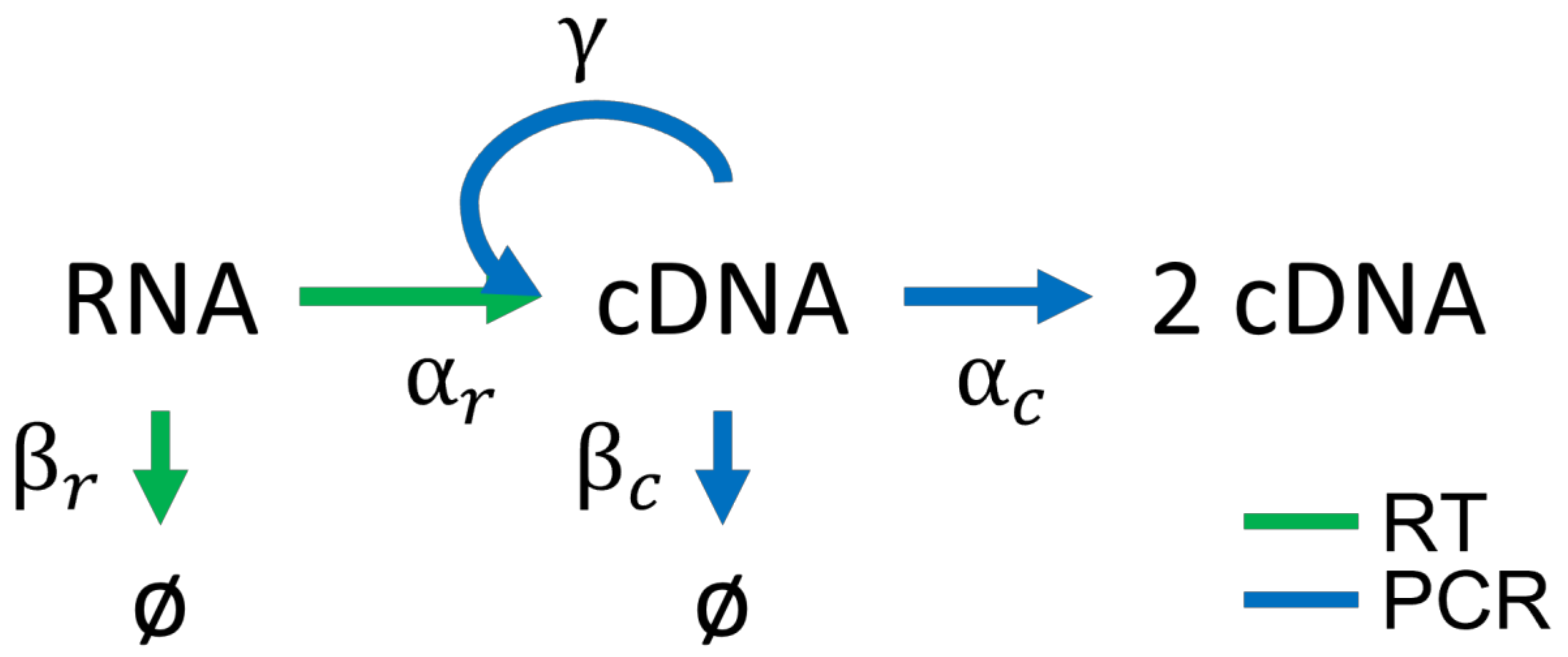
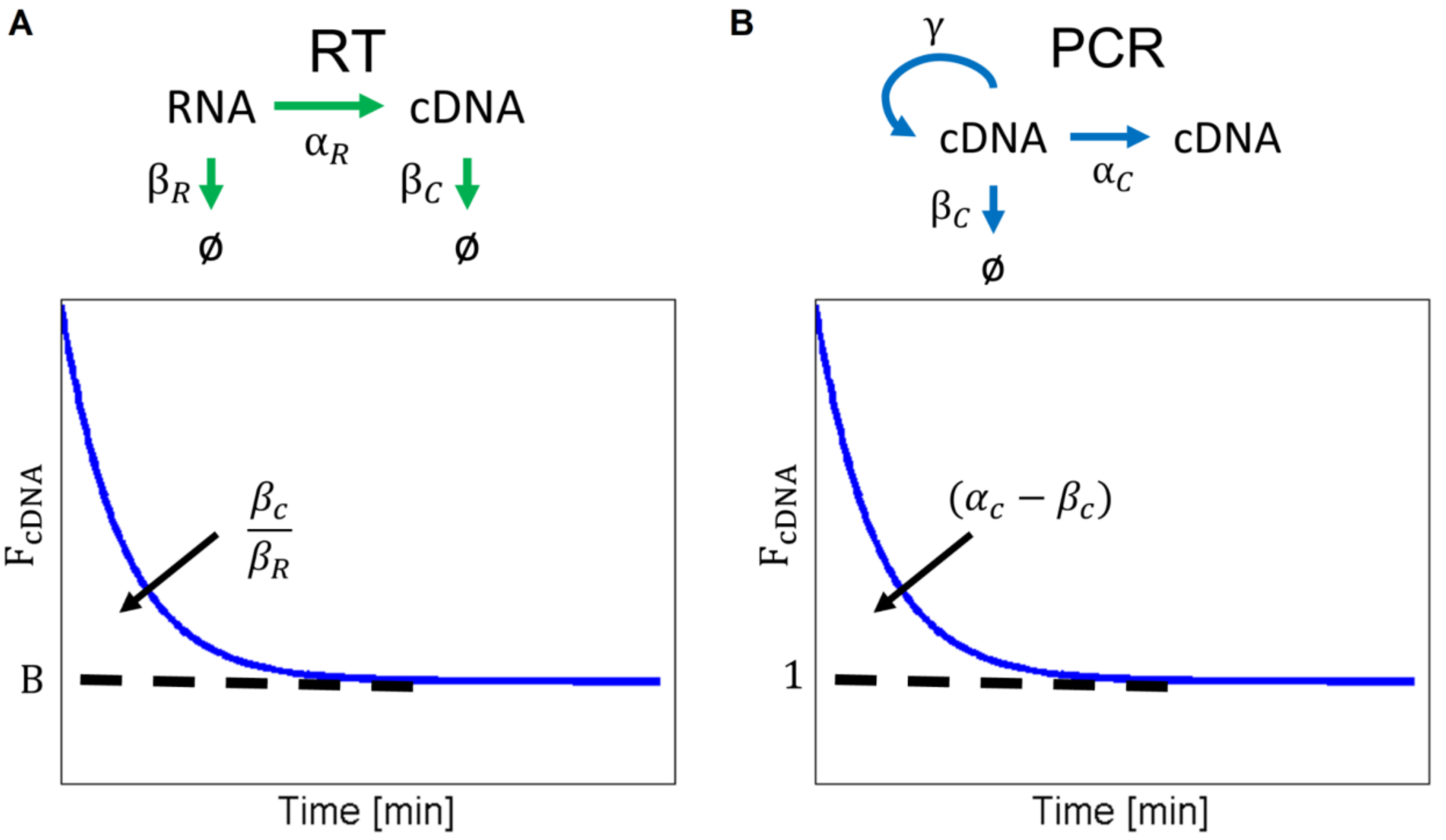
2.1. RT-PCR Model

The RT-PCR is an experimental technique that combines reverse transcription to transform RNA into cDNA and a polymerase chain reaction (PCR) for amplifying a specific cDNA target. Therefore, the complete method integrates two phases. Following the experimental design for the one and two steps RT-PCR, we split the RT-PCR into two coupled processes, the RT and the PCR processes.

Figure 1 depicts a schematic representation of our model; the green and blue arrows differentiate each process. For the RT, cDNA molecules are synthesized by reverse transcription using RNA molecules as templates; the $a_r$ parameter portrays the cDNA synthesis rate held by the activation of the reverse transcriptase. Ideally, the culture medium is RNase-free, so the RNA molecules do not degrade. However, RNA is a labile molecule, and RNases are present everywhere. Therefore, we considered RNA degradation with a rate ${\beta }_r$. Once the reverse transcription is successfully carried on, the cDNA is stable and hardly degraded by enzymes. Moreover, we included the scenario of cDNA loss by enzymatic effect or human manipulation errors with the parameter ${\beta }_c$. In the PCR, the exponential amplification of the cDNA takes place. A cDNA duplication represents a successful amplification. The PCR runs under temperature cycles in which the polymerase activity changes, impacting the cDNA replication rate ($a_c$) (see Section 2.4). Again, we considered a possible cDNA loss by the parameter ${\beta }_c$; finally, in some cases, the complete cDNA strand cannot be appropriately amplified due to errors or temperature changes in the cycle, so the cDNA count does not change. We represent this scenario with the parameter $\gamma$. We coupled both processes by taking the cDNA final value in the RT step as the initial value for the PCR step.

2.2. Chemical Master Equation

Given that the concentration of RNA in one cell is of nanomoles, amplification of cDNA by real-time PCR is governed by random biochemical processes. At a molecular level, random events of gains and inconsistent cDNA amplification contribute to this stochasticity. Although variability was considered to describe the PCR efficiency [9,10], a stochastic approach based on CME has not been used to model the RT-PCR. To do so, we modeled the RT-PCR as a set of biochemical reactions portraying the main steps. Every reaction represented a Markov process derived from the stochastic chemical reaction kinetics [11,12]. We considered a fixed reaction volume in thermal equilibrium with n different chemical species homogeneously distributed. Furthermore, we assumed that molecules collide randomly and chemical reactions occur at random times in a well-mixed space. The CME governs the evolution of the probability distribution of the chemical species given a reaction network. Therefore, the CME positively determines all conditions that lead to the n state minus the possible reactions that take the system out of the n state. The generalization of the CME is presented as follows:

$$\frac{d}{dt}p\left(n,t\right)={\displaystyle \sum }_{i=1}^m\left(p\left(n-d_i,t\right)f_i\left(n-d_i\right)-p\left(n,t\right)f_i\left(n\right)\right),$$

(1)

where $p\left(n,t\right)$ defined the distribution probability for the molecular count n of random variables at time $t$. $f$ is the associated propensity function (occurrence probability for each reaction) for a specific state for the possible i reactions. The associated propensity $f_i\to ℝ\ge 0$ and has the form

$$f_i={\gamma }_i{\displaystyle {{\displaystyle \prod }}_{j=1}^n}\left(\begin{array}{c}{x}_j\\ l_j\end{array}\right),$$

(2)

${\gamma }_i$ is the reaction rate of the reaction $i$. ${{\displaystyle \prod }}_{j=1}^n\left(x_j{l}_j\right),$ equals the number of all distinct reactant combinations taking part in the reaction $i$.

To proceed with the stochastic model, we conceptualized Figure 1 into a set of coupled chemical reactions with an associated propensity. Since all the reactions are first-order, the propensities are the multiplication of the reaction rate and the reactant concentration [13],

Table 1. Reactions, propensities and parameter values for the stochastic model.

Reaction	Propensities	Parameter Value	Description
Reverse Transcription
$RNA\stackrel{{\alpha }_R}{\to }cDNA+RNA$	${\alpha }_{R}RNA$	${\alpha }_R=0.6 {\min }^{-1}$	Reverse transcription.
$RNA\stackrel{{\beta }_R}{\to }\varnothing$	${\beta }_{R}RNA$	${\beta }_R=1.0 {\min }^{-1}$	Degradation of one RNA molecule.
$cDNA\stackrel{{\beta }_C}{\to }\varnothing$	${\beta }_{C}cDNA$	${\beta }_C=0.01 {\min }^{-1}$	Degradation of one cDNA molecule.
Polymerase Chain Reaction
$cDNA\stackrel{{\alpha }_c}{\to }2cDNA$	${\alpha }_C\left(T\right)cDNA$	Equation (5)	Synthesis of one cDNA molecule.
$cDNA\stackrel{\gamma }{\to }cDN{A}^{*}+cDNA$	$\gamma cDNA$	$\gamma =10 {\min }^{-1}$	Deficient synthesis of one cDNA molecule
$cDNA\stackrel{{\beta }_C}{\to }\varnothing$	${\beta }_{C}cDNA$	${\beta }_C=0.01 {\min }^{-1}$	Degradation of the cDNA.

. Therefore, two random variables defined the state of the system: the counts of RNA and cDNA strands.

We formulated the CME for the RT and PCR processes separately, defining the change in the probability distribution over time for the number of RNA and cDNA molecules. Both equations are presented as follows:

$$\begin{array}{c}\frac{d}{dt}p\left(N_{RNA},N_{cDNA},t\right)\hfill \\ \hspace{1em}\hspace{1em}\hspace{1em}\hspace{1em}\hspace{1em}\hspace{1em}={\alpha }_R{N}_{RNA}p\left(N_{RNA},N_{cDNA}-1,t\right)+{\beta }_R(N_{RNA}\hfill \\ \hspace{1em}\hspace{1em}\hspace{1em}\hspace{1em}\hspace{1em}\hspace{1em}+1)p\left(N_{RNA}+1,N_{cDNA},t\right)+{\beta }_C(N_{cDNA}\hfill \\ \hspace{1em}\hspace{1em}\hspace{1em}\hspace{1em}\hspace{1em}\hspace{1em}+1)p\left(N_{RNA},N_{cDNA}+1,t\right)\hfill \\ \hspace{1em}\hspace{1em}\hspace{1em}\hspace{1em}\hspace{1em}\hspace{1em}-\left({\alpha }_R{N}_{RNA}+{\beta }_R{N}_{RNA}+{\beta }_C{N}_{cDNA}\right)p\left(N_{RNA},N_{cDNA},t\right),\hfill \end{array}$$

(3)

$$\begin{array}{c}\frac{d}{dt}p\left(N_{cDNA},t\right)={\alpha }_C(N_{cDNA}-1)p\left(N_{cDNA}-1,t\right)+{\beta }_C(N_{cDNA}\hfill \\ \hspace{1em}\hspace{1em}\hspace{1em}\hspace{1em}\hspace{1em}\hspace{1em}+1)p\left(N_{cDNA}+1,t\right)-\left({\alpha }_C{N}_{cDNA}+{\beta }_C{N}_{cDNA}\right)p\left(N_{cDNA},t\right),\hfill \end{array}$$

(4)

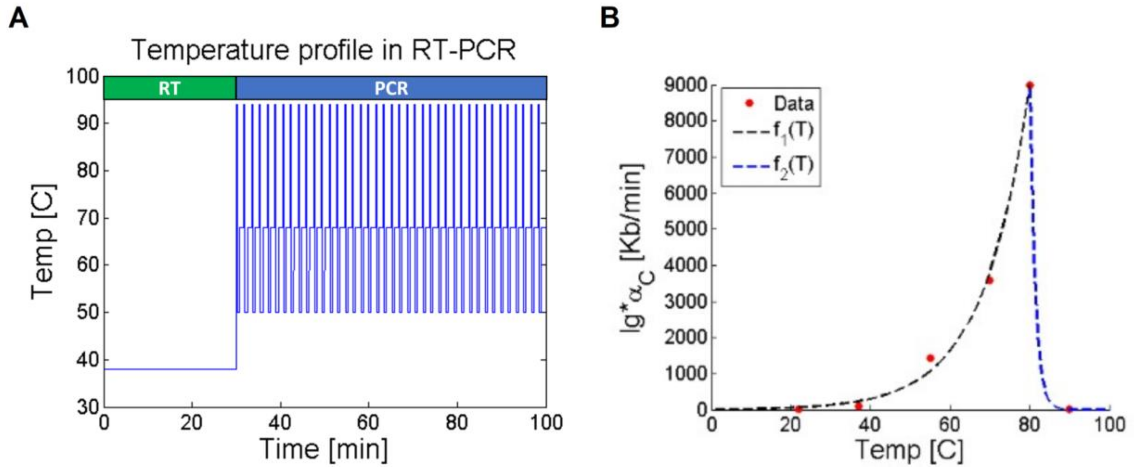
2.3. Parameter Values

The reverse transcriptase is the enzyme that carries the conversion from mRNA to cDNA. Several commercial enzymes have speed ranges from 0.125 kilobases per minute (Kb/min) to 1.2 Kb/min (according to the manufacturer ThermoFisher). Based on this speed and considering a generic transcript of 2 kilobases (Kb), we used an activation parameter (${\alpha }_r$) equal to $1.2 \mathrm{Kb}\ast {\min }^{-1}/2 \mathrm{Kb}=0.6 {\min }^{-1}$. For the RNA degradation rate (${\beta }_r$), experimental evidence revealed that over a pool of 50 tested genes, almost 80% of their RNAs have a half-life (${\tau }_{1/2}$) of less than two minutes [14]. Taking into account this observation, we chose an RNA ${\tau }_{1/2}=0.7 \min$. Consistently with our estimation, RNA${\tau }_{1/2}$ numeric value is in the range of the experimental evidence [14]. Among eukaryotes and prokaryotes, RNA degradation is considered a first-order reaction [15,16]. Therefore, the degradation rate was calculated as follows: ${\beta }_r=In2/{\tau }_{1/2}=1 {\min }^{-1}$. Contrary to RNA, cDNA is a stable molecule hardly degraded by enzymes. Notwithstanding, cDNAses are present in the samples. Therefore, to consider a possible cDNA degradation event with a low rate (${\beta }_c$), we assumed a value of $0.01 {\min }^{-1}$. Finally, $\gamma$ represents the occurence of an incomplete cDNA synthesis due to external factors such as the abrupt changes in the temperature. For this parameter, there is no experimental quantification yet, so we proposed a value of $10 {\min }^{-1}$.

2.4. Temperature Considerations

The RT-PCR relies on the temperature change to control reverse transcriptase and cDNA amplification. The dynamic behavior of the temperature along the process is shown in Figure 2A. Given the experimental protocols from the New England Biolabs inc^® (https://international.neb.com/, accessed on 15 May 2021), we contemplated the temperature for every step in each phase. For the RT phase, the temperature is constant at 38 °C for 30 min, so the RNA template is converted into cDNA by the enzyme reverse transcriptase. Once the cDNA is synthesized, it is amplified in the PCR phase. During this last step, the temperature changes in a stepwise cyclic fashion of three steps: (1) denaturation, double-stranded cDNA are heated at 93 °C to separate the strand; (2) annealing, in which single-strand cDNA is heated at 50 °C to bind the primers to the target regions; (3) extension, at 68 °C the DNA polymerase extends the primer along the template strands. These three phases are repeated 25–35 times to amplify the target cDNA exponentially. To consider the dynamic behavior of the temperature into our mathematical model, we adjusted the DNA polymerase activity ($a_c$) using a piecewise function according to experimental values, Figure 2B and Equation (5). We took the data from experimental measurements of the Taq DNA polymerase speed [17]. We used a nonlinear least fitting method with an exponential model. Thus, the cDNA transcription rate was described by Equation (5), where T is the temperature and lg is the longitude of the new transcript in the number of bases. The transcripts segments processed via the RT-PCR are between 0.5 and 2 Kb [18]. Therefore, we selected an arbitrary value of 2 Kb; this is acceptable for different RNA-seq applications from noncoding to coding RNA.

$${\alpha }_C\left(T\right)=\left\{\begin{array}{c}{f}_1\left(T\right)=\frac{9.88}{lg}{e}^{\frac{T}{11.75}}T\le 80\\ f_2\left(T\right)=\frac{2.33}{lg}{e}^{-\frac{T}{1.37}}T>80\end{array}\right.,$$

(5)

2.5. Deterministic Solution

To statistically characterize the expression of an amplified gene, we calculated the mean and the variance of the probability distribution described in the CME. As the CME depicts the change over time of the probability distribution, we took the derivative of the mean and variance to use the CME according to the following equations:

$$\langle x\rangle ={\displaystyle {{\displaystyle \sum }}_{i=0}^{\infty }}{x}_{i}p\left(x_i\right),$$

(6)

$$\frac{d}{dt}\langle x\rangle ={\displaystyle {{\displaystyle \sum }}_{i=0}^{\infty }}{x}_i\frac{d}{dt}p\left(x_i\right),$$

(7)

$$Var\left(x\right)={\displaystyle {{\displaystyle \sum }}_{i=0}^{\infty }}{x}_i^{2}p\left(x_i\right)-{\langle x\rangle }^2,$$

(8)

$$\frac{d}{dt}Var\left(x\right)={\displaystyle {{\displaystyle \sum }}_{i=0}^{\infty }}{x}_i^2\frac{d}{dt}p\left(x_i\right)-2\langle x\rangle \frac{d}{dt}\langle x\rangle ,$$

(9)

where $\langle x\rangle$ and $Var\left(x\right)$ are the mean and variance of the random variable ${\mathit{x}}_{\mathit{i}}$, $\frac{\mathit{d}}{\mathit{d}\mathit{t}}\mathit{p}\left({\mathit{x}}_{\mathit{i}}\right)$ is the CME depicted in Equations (2) and (3). In the RT-PCR process, we defined two random variables: the number of RNA and cDNA strains. The mathematical appendix shows the exact solution for Equations (7) and (9) for cDNA counts.

2.6. Simulation

Even though the solution of CME allows identifying the first and second moments of the gene expression distribution, it has limitations when we ask about how the initial concentration of RNA affects the frequency of dropout events. Therefore, to explore this last question, we solved the CME of the stochastic model by Gillespie’s algorithm in python 3. The algorithm idea is to compute two random numbers according to the reaction propensities. The first number sets the waiting time for the subsequent reaction according to a random number with an exponential distribution. The second random number chooses the reaction to occur based on a uniform distribution. Finally, the system is updated according to the reaction rules [19]. Experimental protocols establish that RNases must be added to the sample once RT ends to avoid molecule heterogeneity. Consequently, after the simulation ended the RT step, the number of RNA was zero. We adapted the algorithm to consider the temperature–time dependency on the reaction rates. The complete algorithm is explained in

Table 2. Stochastic simulation algorithm.

1: INPUT: initial time $t_0$, state $x_0$ and final time $T_f$ equal to $76 \min$;

2: SET: $x\leftarrow x_0$ and $t\leftarrow t_0$;

3: WHILE: $t$ less than $T_f$

4:  SET the temperature ($T\left(t\right)$) value according to the Figure 2A profile;

5:  IF: $t$ less than $30 \min$

6:   SET: ${\alpha }_c$ and $\gamma$ equal to zero;

7:  ELSE

8:   SET ${\alpha }_C\left(T\right)$ equal to Equation (5);

9:   SET: $RNA$ count equal to zero;

10:  END IF

11:  DEFINE a as the sum of the propensities;

12:  DETERMINE the next jump τ given a;

13:  DETERMINE the next reaction to occur given a;

14:  UPDATE the system counts ($x$) and time ($t$);

15: END WHILE

. Simulation time was 76 min over 1000 independent realizations for every condition.

3. Results

The RNAseq portrays the transcriptome comprising messenger RNA by a single or a collection of cells under a biological condition. Transcriptome studies decode gene functions revealing their regulatory and molecular mechanisms. Although the single-cell RNA-seq portrays the transcriptional landscape, it is subject to errors leading to possible misinterpretations. One origin of these errors is the low initial RNA counts before the RT-PCR that induce zero-inflated data. In addition, the RT-PCR is subject to intrinsic stochasticity affecting the final amplification efficiency. The inherent noise obligated us to evaluate the fundamental question of whether a lower count reflects a biological condition or is just an artifact of the method. To elucidate how the different noise sources could affect the frequency of dropout events in the RT-PCR, in the following sections, we discuss the solution of the CME (Equations (3) and (4)) obtained from numerical and analytical descriptions. As expected, both cases converge and contribute to understanding how noise modulates gene expression in the single-cell RNA-seq technology.

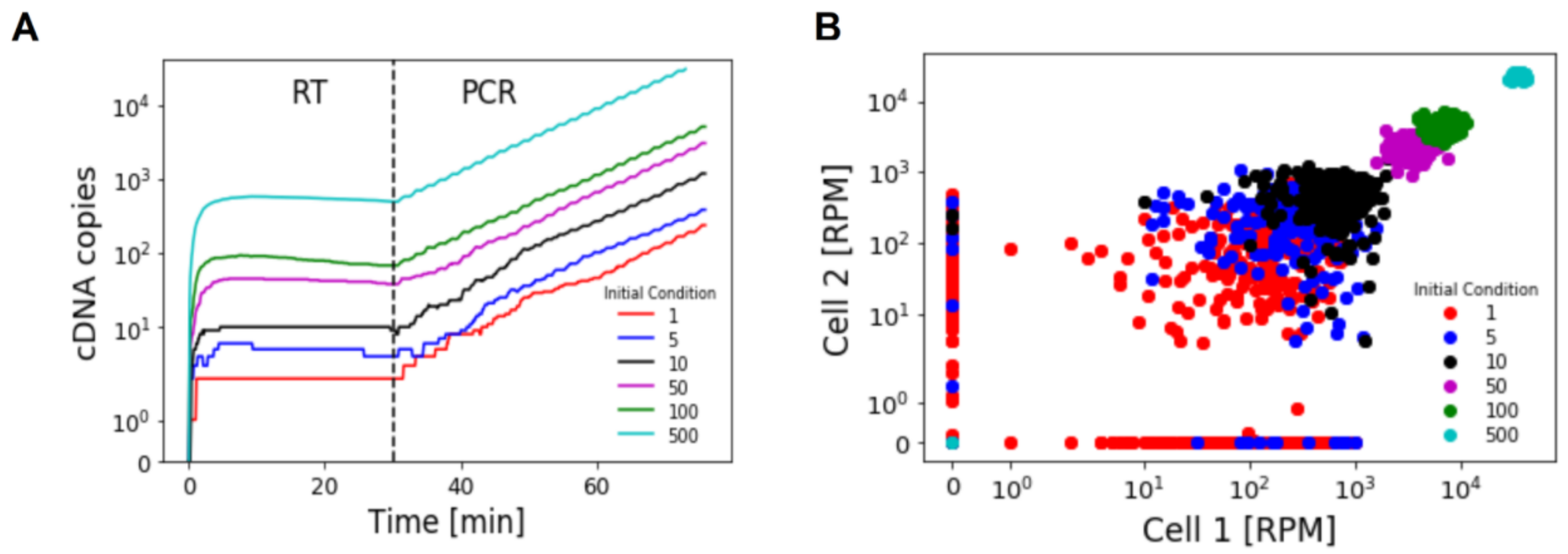
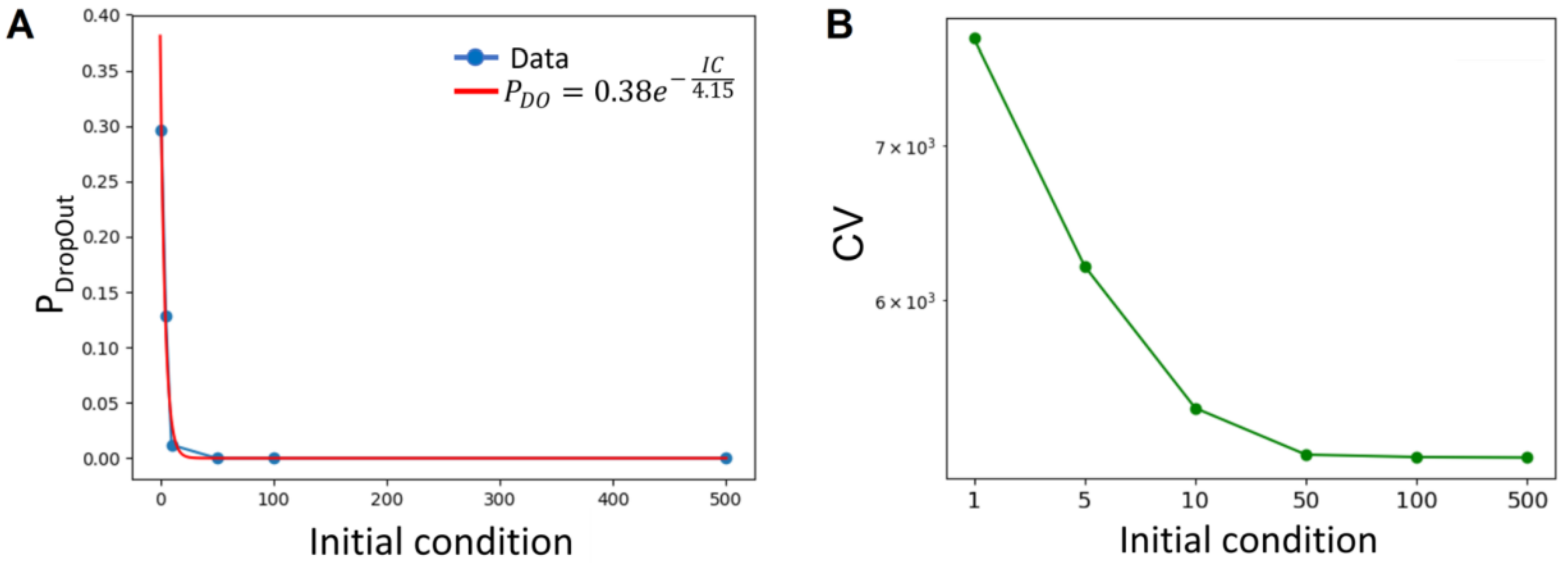
3.1. Numerical Solution of CME

As we have highlighted previously, the single-cell RNAseq measurements are sparse and have uncertainty associated. Therefore, it is more practical to take a probabilistic perspective to study the underlying expression state. Thus, using a stochastic framework, we modeled the RT-PCR as a stochastic process with discrete states (Figure 1 and Equations (3) and (4)). The observable stochastic effect is the occurrence of dropout events related to RNA concentrations. Nevertheless, the prior expression distribution cannot be quantified experimentally. To study the relationship between the dropout occurrence and RNA initial values, we used six discrete initial RNA values ranging from low to high initial counts (1, 5, 10, 50, 100, and 500). The CMEs were solved using the Gillespie algorithm for 76 min for the different initial conditions assuming an isogenic cell population (Figure 3A). To validate the feasibility of the stochastic model, we considered two identical but independent cells with the same number of RNA molecules and initial conditions. Thus, we solved the model for each cell and initial condition over 1000 realizations. By comparing the final value of cDNA for both cells, we observed two significant characteristics (Figure 3B). First, as the initial values of RNA increase, the cDNA copies are higher and have less dispersion; additionally, the cells get more correlated between them, showing an alignment to the 45° line. For lower RNA initial values, cells are less correlated, showing more dispersion. Second, there are vertical and horizontal aligned points with a 0 value for one of the cells. Therefore, in a borderline condition, one cell successfully amplifies the cDNA while the other does not. The appearance of these lines is the graphical representation of the dropout events. In agreement with previous reports [3], our in silico model qualitatively reproduced the typically funnel expression patterns observed for single-cell RNA-seq data. We took single-cell data previously reported from an isogenic three-dimensional tumor model to reinforce the validation further. We carried out the scatter plot for gene expression in two arbitrary cells [4]. As Figure 3B and Figure 4 show, the expression distribution was qualitatively reproduced by our computational analysis. Therefore, the number of dropout events seems to be inversely related to the RNA initial value.

Dropout events portray the technical noise by missing non-zero RNA entries as zero. To describe the dependence between the dropout occurrence and the RNA initial value, we computed the dropout probability (P_DO) by the ratio of the number of realizations that ended in cDNA zero value by the total number of realizations (Figure 5A). Blue dots represent the P_DO values, as the continuous line is the fitted equation (Figure 5A). Therefore, dropout occurrence decreases as the RNA concentration increases. We observed that P_DO exponentially decays and is practically 0 at an initial value of 10. Consequently, it appears that amplification can be adequate even for lower RNA initial values.

In addition, we observed a decrease in the dispersion for higher RNA initial values (Figure 3B). To study the association of the dispersion and the RNA initial values, we evaluated the dispersion by the coefficient of variation (CV) for every initial condition (IC). The CV has a similar tendency as the P_DO; it decreases as the initial RNA value increases (Figure 5B). Interestingly, for IC values greater than 10 molecules, the CV asymptotically reaches a non-zero value. This result implies that there is a limit in the dispersion reduction based on the IC. It seems that the stochastic nature of the RT-PCR always induces an inherent amount of variability in the measurement.

3.2. Analytical Description

Simulated results depicted the effect between the initial RNA counts and the cDNA final values. In addition, we studied the parameter sensitivity of the model relative to the dispersion induction. The observable variable at the end of the RT-PCR is the cDNA. Thus, we deducted the Fano factor for the number of cDNA copies (F_cDNA). The Fano factor measures the dispersion of a probability distribution; it is defined as the ratio of the variance to the mean. To do so, we analytically solved the CMEs (Equations (3) and (4) for the mean and variance (Mathematical Appendix)). Equations (10) and (11) describe F_cDNA for the RT and PCR phases, respectively;

$$\begin{array}{c}{F}_{cDNA}=\frac{e^{-{\beta }_R*t}}{e^{-{\beta }_R*t}-e^{-{\beta }_c*t}}+\frac{\left[2-{\alpha }_R{N}_R^0\right]}{{\beta }_R+{\beta }_c}\frac{e^{-({\beta }_R+{\beta }_c)t}}{e^{-{\beta }_R*t}-e^{-{\beta }_c*t}}\hfill \\ \hspace{1em}\hspace{1em}\hspace{1em}\hspace{1em}\hspace{1em}+\frac{\left[2-{\alpha }_R{N}_R^0\right]}{2{\beta }_c}\frac{e^{-\left(2{\beta }_c\right)t}}{e^{-{\beta }_R*t}-e^{-{\beta }_c*t}}-\frac{1}{{\beta }_c}\frac{e^{-\left(2{\beta }_R\right)t}}{e^{-{\beta }_R*t}-e^{-{\beta }_c*t}}\hfill \\ \hspace{1em}\hspace{1em}\hspace{1em}\hspace{1em}\hspace{1em}-\frac{{\beta }_C}{{\beta }_R}\frac{e^{-\left(2{\beta }_R\right)t}}{e^{-{\beta }_R*t}-e^{-{\beta }_c*t}}\hfill \end{array}$$

(10)

$$\begin{array}{c}\hfill F_{cDNA}=N_{cDNA}^0{e}^{-({\alpha }_c-{\beta }_R)T}-N_{cDNA}^0+\frac{{\alpha }_c+{\beta }_R}{{\alpha }_c-{\beta }_R}-\frac{{\alpha }_c+{\beta }_R}{{\alpha }_c-{\beta }_R}{N}_{cDNA}^0{e}^{-({\alpha }_c-{\beta }_R)T}\hfill \\ \hfill +Var{\left(cDNA\right)}^0{e}^{-({\alpha }_c-{\beta }_R)T}.\hfill \end{array}$$

(11)

where $N_R^0$ is the initial value for RNA before the RT phase. $N_{cDNA}{}^0$ is the initial value for cDNA before the PCR phase.

Plotting previous equations exhibit the dispersion dependence on the model parameters (Figure 6). For the RT phase, $F_{cDNA}$ exponentially decays to $B\propto 1/\left({\beta }_r+{\beta }_c\right)$. The decay speed depends on the ratio of the RNA and cDNA degradation rates, ${\beta }_r$ and ${\beta }_c$. As the ratio increases, the system needs more time to reach its steady-state (Figure 6A). The presence of a non-zero steady-state is intriguing since variability will prevail. The $F_{cDNA}$ has similar dynamics regarding the PCR phase but with a more intuitive regulation. The difference between the amplification rate sets the decay speed (${\alpha }_c$) and cDNA degradation rate (${\beta }_c$) (Equation (11) and Figure 6B). The $F_{cDNA}$ for this phase has an asymptotic value of 1. At the steady-state, the variance is equal to the mean being the lowest possible dispersion value. Thus, although the noise will always be present, it can be limited. In summary, these results suggest that the noise-limiting factor is the RNA degradation rate.

4. Discussion

Quantification of RNA among different conditions has turned into a standard to understand and unravel gene regulation. RT-PCR mimics the basic process of DNA replication within cells and constitutes an essential component to extract the gene expression profile in single-cell RNAseq. From the experimental point of view, RT-PCR relies on temperature cycles to trigger enzymatic chemical reactions to quantify RNA based on its conversion to cDNA. Although theoretically, the cDNA at least doubles its amount after each amplification cycle. Data show varying yields and errors suggesting inner random processes increased at low RNA initial concentrations. Hence, we proposed an RT-PCR stochastic model portraying the inherent molecular stochasticity and experimental errors. We focused on the characterization of the dropout events and the variability induction. To this end, we explored the dropout events dependence within the initial RNA values by numerically solving the chemical master equation. In addition, we evaluated the limits in the variability reduction.

Despite our simple RT-PCR stochastic representation, we reproduced expression patterns from single-cell RNA-seq data observed in different cell types and experimental conditions [3,4,20]. Notably, we found a threshold that restricts the minimal amount of processed RNA without bias by zero-inflated data due to dropouts. Based on the parameters used in this paper, this limit is around 10–50 RNA copies. As intuitively expected, our model suggests that error events decrease with the initial RNA copy number increase. Furthermore, quantification of rare transcripts (transcripts with low copies) pushes the measurements to a point where the output distribution reflects biological information and noise. However, if those rare transcripts are present in low amounts but surpass the null dropout occurrence threshold, the data would associate those transcripts to trustworthy biological processes. Hence, genes with low gene expression can keep their biological information relative to other genes.

Data correction is a widely used strategy to subtract the dropouts bias. However, imputation and assuming non-verified prior expression distribution are tools to be used carefully. Imputation techniques rely on the existence of a reference distribution, and when there is not one, it is inferred. This circular logic induces false positives and an increase in the correlation between genes. These problems become apparent for non-characterized cell populations and cells closely related. In terms of experimental strategies to overcome dropouts, spike-ins quantify amplification efficiency to perform data correction. Nevertheless, despite their accuracy, they can dim genes’ internal expression and vary even between technical replicates [21,22]. Given our results, dropout reduction is possible by increasing the RNA initial counts. However, controlling RNA initial values seems a non-feasible task. In addition, manipulation of the prior RNA expression distribution might induce bias leading to misinterpretation of the biological scenario. Therefore, we proposed that instead of modifying RNA initial counts, dropout occurrence can diminish by controlling the experimental conditions.

Otherwise, it is important to mention that the CME for the PCR phase does not include the cDNA deficient synthesis portrayed by γ. Initially, we hypothesized that the induced errors by this reaction restrain the efficiency of the process. Although deficient amplification does not modify the molecular count or the probability distribution, our results revealed that degradation processes are the primary error inducer.

Along with the threshold existence, there is a basal variability despite the initial RNA values. The analytical description showed that the total variability becomes constant as the RNA values increase. As expected, the total data dispersion comprises two effects: the inherent stochasticity of the chemical reaction and the errors induced by dropouts. It seems that variability induction and propagation are inherently immovable. Hence, the biological variability might be obscured by RT-PCR inherent dispersion, leading to biased results and relations. This suggests implementing additional considerations to improve the statistical analysis, further than imputing the dropout variability.

Instead of performing simulation with changes in the values of model parameters, we evaluated the parameter sensitivity solving the CMEs analytically. The Fano factor depicts the effect on the parameters into the dispersion dynamics. In general terms, stochasticity cannot be eradicated. In every process, it has a non-zero minimum. The property that can be modified is the decay speed to reach the minimum. Interestingly, toward the RT phase, the dispersion decay is modulated by the degradation parameters ratio. The parameter to attend is the RNA degradation rate; it is the most sensitive and challenging variable to diminish noise. Therefore, this parameter is the limiting factor for experimental noise propagation and variability induction. RNA degradation rate can decrease by controlling the presence of RNases. While RNase contamination can result in a failed experiment, it is difficult to determine the contamination origin. Nevertheless, there are alternatives to diminish the contamination probability. Experimental protocols allow removing RNases from plastic, inhibiting RNases by enzymes, getting RNase-free solutions, and not propagating RNases contamination [23].

For the PCR phase, the decay speed can increase by increasing the cDNA replication rate. As the experimental techniques evolve, new Taq polymerases arise with higher speed and replication quality. Therefore, the replication rate is increasing with the technology. The cDNA degradation rate might not be a relevant variable due to cDNA molecule stability.

We conclude that the RT phase is the most critical step to be susceptible to noise and consequently the primary source of dropout events in single-cell RNAseq. Therefore, we propose a synergic strategy based on experimental dropout reduction and posterior data correction.

References

1. Wang, Z.; Gerstein, M.; Snyder, M. RNA-Seq: A revolutionary tool for transcriptomics. Nat. Rev. Genet. 2009, 10, 57–63. [Google Scholar] [CrossRef] [PubMed]
2. Kashima, Y.; Sakamoto, Y.; Kaneko, K.; Seki, M.; Suzuki, Y.; Suzuki, A. Single-cell sequencing techniques from individual to multiomics analyses. Exp. Mol. Med. 2020, 52, 1419–1427. [Google Scholar] [CrossRef] [PubMed]
3. Kharchenko, P.V.; Silberstein, L.; Scadden, D.T. Bayesian approach to single-cell differential expression analysis. Nat. Methods 2014, 11, 740–742. [Google Scholar] [CrossRef] [PubMed]
4. Muciño-Olmos, E.A.; Vázquez-Jiménez, A.; De León, U.A.-P.; Matadamas-Guzman, M.; Maldonado, V.; López-Santaella, T.; Hernández-Hernández, A.; Resendis-Antonio, O. Unveiling functional heterogeneity in breast cancer multicellular tumor spheroids through single-cell RNA-seq. Sci. Rep. 2020, 10, 12728. [Google Scholar] [CrossRef] [PubMed]
5. Robert, C.; Watson, M. Errors in RNA-Seq quantification affect genes of relevance to human disease. Genome Biol. 2015, 16, 177. [Google Scholar] [CrossRef] [PubMed] [Green Version]
6. Laehnemann, D.; Köster, J.; Szczurek, E.; McCarthy, D.; Hicks, S.; Robinson, M.D.; Vallejos, C.; Campbell, K.; Beerenwinkel, N.; Mahfouz, A.; et al. Eleven grand challenges in single-cell data science. Genome Biol. 2020, 21, 31. [Google Scholar] [CrossRef]
7. Andrews, T.S.; Hemberg, M. False Signals Induced by Single-Cell Imputation. F1000Research 2018, 7, 1740. [Google Scholar] [CrossRef] [PubMed]
8. Kharchenko, P.V. The triumphs and limitations of computational methods for scRNA-seq. Nat. Methods 2021, 18, 723–732. [Google Scholar] [CrossRef] [PubMed]
9. Alvarez, M.J.; Vila-Ortiz, G.J.; Salibe, M.C.; Podhajcer, O.L.; Pitossi, F.J. Model based analysis of real-time PCR data from DNA binding dye protocols. BMC Bioinform. 2007, 8, 85. [Google Scholar] [CrossRef]
10. Pfaffl, M.W. A new mathematical model for relative quantification in real-time RT-PCR. Nucleic Acids Res. 2001, 29, e45. [Google Scholar] [CrossRef] [PubMed]
11. Van Kampen, N.G. Stochastic processes. In Stochastic Processes in Physics and Chemistry, 3rd ed.; Elsevier: Amsterdan, The Netherlands, 2007; pp. 52–72. ISBN 9780444529657. [Google Scholar]
12. Gillespie, D.T. Jump Markov processes with discrete states. In Markov Processes: An Introduction for Physical Scientists; Academic Press: San Diego, CA, USA, 1992; pp. 317–373. [Google Scholar] [CrossRef]
13. Gillespie, D.T. A general method for numerically simulating the stochastic time evolution of coupled chemical reactions. J. Comput. Phys. 1976, 22, 403–434. [Google Scholar] [CrossRef]
14. Baudrimont, A.; Voegeli, S.; Viloria, E.C.; Stritt, F.; Lenon, M.; Wada, T.; Jaquet, V.; Becskei, A. Multiplexed gene control reveals rapid mRNA turnover. Sci. Adv. 2017, 3, e1700006. [Google Scholar] [CrossRef] [PubMed] [Green Version]
15. Laguerre, S.; González, I.; Nouaille, S.; Moisan, A.; Villa-Vialaneix, N.; Gaspin, C.; Bouvier, M.; Carpousis, A.J.; Cocaign-Bousquet, M.; Girbal, L. Large-Scale Measurement of mRNA Degradation in Escherichia coli: To Delay or Not to Delay. Methods Enzymol. 2018, 612, 47–66. [Google Scholar] [CrossRef] [PubMed]
16. Chen, C.A.; Ezzeddine, N.; Shyu, A. Chapter 17 Messenger RNA Half-Life Measurements in Mammalian Cells. Methods Enzymol. 2008, 448, 335–357. [Google Scholar] [CrossRef] [PubMed] [Green Version]
17. Innis, M.A.; Gelfand, D.H.; Sninsky, J.J.; White, T.J. PCR Protocols: A Guide to Methods and Applications; Academic Press: Cambridge, MA, USA, 2012; ISBN 9780080886718. [Google Scholar]
18. Poulin, N.M.; Nielsen, T.O. Expression arrays: Discovery and validation. In Cell and Tissue Based Molecular Pathology; Churchill Livingstone: London, UK, 2009; pp. 70–83. ISBN 9780443069017. [Google Scholar]
19. Gillespie, D.T. Exact stochastic simulation of coupled chemical reactions. J. Phys. Chem. 1977, 81, 2340–2361. [Google Scholar] [CrossRef]
20. Wohnhaas, C.T.; Leparc, G.G.; Fernandez-Albert, F.; Kind, D.; Gantner, F.; Viollet, C.; Hildebrandt, T.; Baum, P. DMSO cryopreservation is the method of choice to preserve cells for droplet-based single-cell RNA sequencing. Sci. Rep. 2019, 9, 10699. [Google Scholar] [CrossRef] [PubMed] [Green Version]
21. Vallejos, C.; Risso, D.; Scialdone, A.; Dudoit, S.; Marioni, J.C. Normalizing single-cell RNA sequencing data: Challenges and opportunities. Nat. Methods 2017, 14, 565–571. [Google Scholar] [CrossRef] [PubMed]
22. Risso, D.; Ngai, J.; Speed, T.P.; Dudoit, S. Normalization of RNA-seq data using factor analysis of control genes or samples. Nat. Biotechnol. 2014, 32, 896–902. [Google Scholar] [CrossRef] [PubMed] [Green Version]
23. Sambrook, J.; Russell, D.W. The Condensed Protocols from Molecular Cloning: A Laboratory Manual; Cold Spring Harbor Laboratory Press: New York, NY, USA, 2006; ISBN 9780879697716. [Google Scholar]
Figure 1. RT-PCR model. Representation of the complete RT-PCR process that was split into two subprocesses. Green and blue arrows denote the RT and the PCR processes, respectively.
Mathematics 09 02515 g001
Figure 2. Temperature dynamic. (A) Temperature profile for the RT and PCR phases. In the PCR, the temperature changes according to three cyclic values (93, 50, and 68 °C). (B) Fitted data to model the DNA polymerase activation speed ( α c ) in function of the temperature (R2 = 0.99 using the nonlinear least squares method). The polymerase speed units are kilobases per minute (Kb/min), and lg is the transcript longitude in number of bases. For each segment, we used a one term exponential model ( A e T / B ). Dots represent experimental values [17], and the discontinued lines are the fitted piecewise function comprising two segments (Equation (5)).
Mathematics 09 02515 g002
Figure 3. Simulation results. (A) Numerical solution of CME for the number of cDNA copies (Equation (4)) considering the RT, and PCR phases, the simulation time was 76 min. Each color line stands for a different initial RNA count before the RT-PCR process. (B) Scatter plot of cDNA copies for two cells that have the same CMEs. For each condition, we performed 200 realizations; the plotted value is the last for the number of cDNA copies at 76 min. The different colors are the initial cDNA count for every point. The expression values for the transcripts are in reads per million (RPM).
Mathematics 09 02515 g003
Figure 4. Data validation. A scatter plot of two isogenic cells from a single-cell study of a breast cancer tumor model [4]. The cells were arbitrarily chosen given the open-access expression matrix. The expression values for the transcripts are in reads per million (RPM).
Mathematics 09 02515 g004
Figure 5. Errors and noise analysis. (A) DropOut probability (PDO) dependency on the RNA initial condition. The computed PDO values (blue dots) for the different initial conditions; the continuous red line is the exponential fitted equation describing the observed points. IC stands for the initial RNA value. The legend shows the value of the parameter with an R2 = 0.99, we used the nonlinear least squares method using an exponential fitting model. (B) Coefficient of variation (CV) for the different initial conditions.
Mathematics 09 02515 g005
Figure 6. (A) Fano factor of the cDNA copies ( F cDNA ) for the RT phase as described by Equation (10). The discontinuous line represents the asymptotic value proportional to 1 / β r + β c . The arrow indicates the increase in the decay speed as the ratio of the degradation rates ( β c / β r ) increases. (B) F cDNA time dynamics for the PCR phase described by Equation (11). The decay speed decreases as the difference in the cDNA replication rate and degradation rate α c β c increases (arrow). The used parameters to draw the F cDNA dynamics are in Table 1.
Mathematics 09 02515 g006