Article

Investigation of Drift Phenomena at the Pore Scale during Flow and Transport in Porous Media

1
School of Engineering, University of Aberdeen King’s College, Aberdeen AB24 3FX, UK
2
Department of Petroleum Engineering, University of Ibadan, Ibadan 200284, Nigeria
*
Author to whom correspondence should be addressed.
Mathematics 2021, 9(19), 2509; https://doi.org/10.3390/math9192509
Submission received: 7 September 2021 / Revised: 22 September 2021 / Accepted: 27 September 2021 / Published: 7 October 2021

Abstract

:
This paper reports an analytical study conducted to investigate the behaviour of tracers undergoing creeping flow between two parallel plates in porous media. A new coupled model for the characterisation of fluid flow and transport of tracers at pore scale is formulated. Precisely, a weak-form solution of radial transport of tracers under convection–diffusion-dominated flow is established using hypergeometric functions. The velocity field associated with the radial transport is informed by the solution of the Stokes equations. Channel thickness as a function of velocities, maximum Reynolds number of each thickness as a function of maximum velocities and concentration profile for different drift and dispersion coefficients are computed and analysed. Analysis of the simulation results reveals that the dispersion coefficient appears to be a significant factor controlling the concentration distribution of the tracer at pore scale. Further analysis shows that the drift coefficient appears to influence tracer concentration distribution but only after a prolonged period. This indicates that even at pore scale, tracer drift characteristics can provide useful information about the flow and transport properties of individual pores in porous media.

1. Introduction

A thorough understanding of transport processes is significant for various applications in engineering, natural resources (for example waste management [1]) groundwater remediation [2] and porous media during tracer injection experiments in a core samples [3]. Tracer testing has become a highly vital tool in geothermal research, resource management and development. It is used for reinjection research and management, general hydrological studies of subsurface flow and flow rate measurement in pipeline [4]. It acts as the source of information for porous media characterisation, hydrocarbon recovery process and geothermal engineering [5].
Tracers are used to determine preferred flow direction, pore connectivity, flow velocity, dispersivity, heterogeneity of oil and gas reservoirs and residual oil saturation [6,7]. To enhance flow characterisation in porous media, an improved study of tracer transport at pore scale is important because pore-space geometry and topology are the key factors that influence flow and transport phenomena. Therefore, solute transport is significantly impacted by pore-scale heterogeneity found in natural porous media [8].
However, direct observation of pore-scale processes are not possible in the field scale [9]. Transport of tracers in porous media involves complex physical phenomena such as drift which often occur on widely varying scales for instance from a pore level to field level. Further, studies have shown that porous media in which transport takes place are heterogeneous and disordered on a microscopic scale, higher additional mixing is required by order of magnitude than the spreading due to pure molecular diffusion. Such an increase in the spreading of an initially narrow tracer pulse is due to mechanical dispersion.
Tracers introduced into a solvent, for example, water flowing through a porous system, will be exposed to dispersion in both longitudinal and transverse direction due to thermal, Fickian diffusion or drift due to variation of flow velocities within the pores [10]. Linear drift is a phenomenon experienced in subsurface flow and transport processes. It originates as a result of aquifer movement during production/injection in a distant reservoir with which there exist hydraulic connectivity and several factors. This drift of tracer particles in a liquid occurred at a pore scale due to microscopic variation of the fluid flow field [11]. Advancement in reservoir modelling which incorporates tracer partitioning between different phases and drift effect due to production as well as adsorption to grain surface requires adequate knowledge of tracer transport at pore scale [12].
Mass spreading of non-reactive tracers can be described by a combination of molecular diffusion, hydrodynamic dispersion and heterogeneous advection [13]. The hydrodynamic dispersion is usually quantified by the sum of the molecular diffusion and advection components. Many models have been developed to describe the space anomalous behaviour of dispersion coefficients (for example flow through rivulet [14], random capillaries [15]). Al Mukahal et al., 2017 provide a description of long-time Taylor–Aris dispersion of solute by using multiple scales to arrive at the expression of effective diffusivity. However, problems associated with Taylor dispersion in a capillary tube are momentous, i.e possibility of micro-macro duality and their interrelationship among scales manifest [16].
Taylor–Aris further examined a case where after a prolonged period, the concentration of solutes follows regular Gaussian distribution. To date, the majority of these studies have focused primarily on investigating flow and transport phenomena at Darcy’s scale. Attention to a pore-scale investigation of flow and transport of solute under the influence of linear drift is yet to be reported in the literature.

Pore-Scale Radial Diffusion Models with Drift

Dispersion of solutes i.e tracers has wide applications in many fields of study (such as, for example, petroleum engineering, ecological studies and hydrology) and has been a huge subject of theoretical and experimental research.
Figure 1 shows a schematic representation of a chemical tracer injection/extraction test in a porous media system. The drift effect fully manifested due to the microscopic variation of the fluid flow field at a later time during the extraction stage (Figure 1f) [16].
However, a continuing challenge in mathematical and computational modelling is how to capture these mechanisms accurately and to handle them to relevant scales properly [17]. The mechanisms controlling the spreading differ in their behaviour and therefore require detailed nano-scale flow characterisation for accurate and reliable predictions of transport to be made.
To describe flow at pore scale, i.e smaller physical scales where pore and solid space are resolved separately, flow and transport are simulated using more detailed description such as Hagen–Poiseulle or Stokes flow [18]. The most basic approach to computing the spatio-temporal evolution of the concentration of tracers is provided by the advection–diffusion equation. The advection–diffusion equation is a standard approach based on Ficks law and the conservation of mass. It assumes Fickian processes and uses hydrodynamic dispersion coefficient in which the effect of solute mixing and spreading are embedded together [3]. It also uses an average linear velocity for a representative elementary volume and assuming perfectly mixed conditions within a representative elementary volume. However, at the pore scale when the velocity field is not fully sampled, incomplete mixing and spreading may exist at early times [8].
Recently, there has been increased interest in problems that involve moving interfaces at the pore scale [19]. These are problems that are characterised by sharp local gradients and mixing-controlled reactions. A large number of recent studies have explored these issues using pore-scale simulators, in which the geometry of pores-spaces and solid material is explicitly considered and processes are defined at the sub-pore [20]. Tsang and Neretnieks studied the flow and transport of solute through channels. They summarised channelling observations, concepts, and modelling of flow and transport in fractures and networks where preferential flow paths (channelling) take place [21].
Despite the numerous studies of flow and transport of tracers through geological porous media, our understanding still faces a significant challenge. One of the challenges is the observation of drift phenomena at a Darcy or field scale [5,16]. The signatures of drift phenomena affect tracer concentration distribution at field scale as reported in the literature [22]. Analytical model solutions that describe and predict tracer transports at field scale have been obtained in cases where tracer adsorption, non-uniform convection, and variable dispersion manifest [23].
Recently, investigations on closed-form solutions of radial transport of tracer in porous media at field scale have been reported in the literature (e.g., Akanji and Falade [16]). Analytical solutions at field scale have been obtained where variable dispersion coefficient and velocity are solved using Green’s function method (GFM) [24] and in steady-state flow field in a horizontal aquifer caused by a constant rate injection from a well, including the mechanical dispersion and molecular diffusion terms in addition to the retardation and first-order attenuation under a Robin-type boundary condition at the well [25].
Akanji and Falade [16] studied the effect of drift on radial transport of tracers in porous media. We discussed the influence of linear drift and show that drift affects concentration profile for a typical system with non-homogeneous porosity distribution. Falade and Brigham [23] carried out a similar study where they used inverse Laplace transformation to solve radial transport equations in real-time-space.
Despite the recent advances in solving advection–diffusion equations both analytically and numerically, there is yet to be attention on the investigation of drift phenomena at the pore scale. All the previous studies mentioned above have focused on cases where convective velocity and hydrodynamic dispersion function were assumed to be constant, meaning the solute molecules i.e tracers are kinematically and dynamically indistinguishable from mobile phase molecules. However, it is important to note that this assumption is not appropriate for pore-scale flow and transport in porous media. Hence, the need for variable radial dispersion in nonuniform flows under the influence of drift is crucial for accurate description of pore-scale flow and transport Phenomena. To date, an exact solution or closed-form solution to the transport equation at pore scale has not been established for cases where hydrodynamic dispersion is radially distributed, and linear drift predominates. An investigation of drift phenomena at pore scale on fluid flow behaviour in porous media under the influence of linear drift is therefore presented in this work. The drift-velocity is encapsulated into the poiseuille flow velocity field. We establish and solve a novel pore-scale convection–dispersion equation and hydrodynamic dispersion function using the velocity obtained from Equation (1) as shown in Equations (4) and (5). This is the novelty of the work. The resulting radial transport equation is then cast in the form of the Whittaker equation using some set of transformation relations and change of variables. Concentration distribution around the source of the tracer or injected particles is computed from a weak-form numerical solution and used to analyse pore-scale tracer concentration behaviour in tracer injection/extraction experiment in a core sample during enhanced oil recovery processes where the influence of drift may obstruct the fluid flow path.

2. Pore-Scale Fluid Flow and Transport of Tracer Model

We consider the partial differential equations governing the flow of an incompressible Newtonian fluid at the pore scale (Akanji and Chidamoio [26,27]) thus:
ρ v t + ρ v · ( v ) = p + μ 2 v
where the variables μ , ρ , P and v are the viscosity, fluid density, reduced pressure gradient and fluid velocity vector respectively. The analytical solution to the Stokes equation is obtained for velocity fields as described in Appendix A.
To study the spatial, radial, and temporal non-uniformity of tracer-mixing flowing in a channel due to velocity variation of tracers flowing in a mobile phase water, time-dependent tracer concentration distribution is computed by solving the convection–diffusion equation expressed in terms of resident concentration in radial coordinates as (Akanji and Falade [16]):
1 r r r ϕ D C r 1 r r r ϕ v C γ k r + s C = ϕ C t
in Equation (2), D is the hydrodynamic dispersion function, v is the convective velocity at radial position r, C is the concentration of tracers, ϕ is the porosity of the system and γ k r + s is the source or sink term that accounts for phenomena such as tracer adsorption, physical loss or addition of tracer particles and reactions of tracer particles with the mobile fluid phase.
The convective velocity v (m/s) in Equation (2) is decomposed into a drift velocity v d superimposed on a radial flow of injected tracer of strenght q i ( m 3 / s ) .
A steady-state flow with a parabolic profile at every location in the channel is assumed. It implies that the transient acceleration term in Equation (1) goes to zero. The pressure gradient is only in the x-direction (unidirectional) and the plates are motionless. It is also assumed that the velocity vector and the velocity gradient tensor are off-diagonal, implying that the dot product is zero (i.e the second term in Equation (1) goes to zero), we also applied no-slip boundary conditions, since velocity is zero at the lower plate (i.e y = −h) of the channel. At the upper plate (i.e. y = +h), the velocity is zero as well, hence the velocity can be written as:
v = 1 2 μ d p d x h y y
This is a Poiseuille flow velocity, also called creeping flow velocity or weak inertial flow velocity (near zero Reynolds number) in a porous media. In Equation (3), d p d x , represents the average pressure gradient in the direction of the flow, μ represents the dynamic viscosity of the fluid, h is the channel thickness and v is the poiseuille fluid velocity. However, when the flow of tracer is motivated by linear drift, The convective flow velocity equals the poiseuille velocity which comprises linear drift and radial velocity components. Therefore Equation (3) represents the convective velocity that is incorporated into the transport equation. Drazin et al. 2006 [28] presented a classification and exact solutions to the Navier–Stokes equations for plane Poiseuille flow through some non-circular cross-sections.

Pore-Scale Convection–Diffusion Equation

In this section, we present only the key equations relevant to pore-scale convection–diffusion and Taylor–Aris dispersion of solute undergoing creeping flow. Our interest is studying the influence of drift at creeping flow upon small scale transport. Thus, we simplified Equation (2) by substituting the Poiseulle velocity of Equation (3) into it. This yields the dimensionless form of the general pore-scale convection–diffusion equation in Laplace space as (see Appendix B for the derivation of the transport equation under the influence of linear drift):
d 2 ψ d r D 2 + k 2 4 k r D + β p 2 p 2 h y y 2 r D 2 16 μ 2 k r D + β p 2 Φ k r + s r D k r D + β p ψ = 0 .
where the variables are defined as:
D h = D m + D o p 2 μ h y y 2 + α r
D h D = D m + v p D o ω + 1 r D ,
γ = ϕ S m + k l 1 S m S m
Here, ψ is a variable which is a function of ( r D ) , r D is the dimensionless pore radius, k is Whittaker function, h is the channel thickness, y is the vertical distance from centre of the channel to top/bottom parallel plates shown in Figure 2, Φ is the Chromatographic response function, s is a Laplace transform parameter and 2 h is the distance between the parallel plates. The hydrodynamic dispersion D h in Equations (5) and (6) includes contribution from molecular diffusion and mechanical mixing. Further, the quadratic terms in pressure and pore size in Equations (4) and (5) make the solution non-trivial when compared to the Darcy-scale version. Parameter D o is the shear mixing constant in (m) and S m is the saturation of the mobile fluid phase.

3. Mathematical Formulation of Pore-Scale Radial Transport Equation with Linear Drifts

To develop the radial transport equation where linear drift effect can be investigated, the following transformation relations are defined: η = k r D + β , r D = η β 1 k and d η d r D = k d η = k d r D d η d r D = d r D .
However, applying the transformation to Equation (4) gives a pore-scale convection–diffusion equation which can be expressed in the form of the Whittaker equation as:
d 2 ψ d Z 2 + 1 4 + k Z + 1 4 μ 2 Z 2 ψ = 0
Equation (8) is a Kummers differential equation whose solution is known. Detailed transformation and simplification of Equation (4) into the Whittaker 8 can be found in Appendix C.
Where:
μ 2 = p 2 β 2 h y y 2 16 μ 2 k 4
μ = p β h y y 2 4 μ k 2
and:
k = p 2 β h y y 2 16 μ 2 k 4 f s + β ϕ k r + s 2 f s
f s = 1 k p 2 h y y 2 16 μ 2 k 2 + ϕ k r + s k
ξ = 2 k r D + β f s
ξ = 2 η f s

3.1. Formulation of Linear Drift

For this investigation, linear drift is applied as a velocity field v d because it is coordinate-independent, carrying velocity magnitude that acts on every point within the porous system.
The tracers are carried along with the fluid in the channel while spreading due to diffusion. Consequently, the convective velocity of the fluid due to transport at pore scale is described by the Poiseuille velocity calculated from Equation (3) above which decomposes into drift velocity and a radial velocity part of an injected tracer of strength q i around the drift velocity. The convective fluid velocity in the channel system is therefore given by:
v = v d + v p ,
where, v = p 2 μ h y y 2 , v p = α r p , and α = q i 2 π h θ .
Therefore, redefining the following variables from Equation (5) as: k = D m + β p , ϖ = v d c o s θ α , β p = α D o which are described as effective dispersion constant, vorticity of the tracer particles in motion and parameter related to velocity along x-direction.

3.2. Pore-Scale Analytical Solution of Radial Transport Equation with Linear Drift

A detailed solution of the general Whittaker equation can be found in Akanji and Falade [16]. Here, we present the pore-scale analytical solution of the radial transport equation where linear drift component is accounted for. Tracer concentration can now be written as:
C = ξ μ p h y y 2 4 μ k 2 2 a 1 2 + p h y y 2 β 4 μ k 2 e p h y y 2 4 μ 2 k ξ 2 U 1 2 + μ k , 1 + 2 μ , ξ
However, constant of separation ω 2 by recasting the general advection–dispersion equation for the flow of tracers with embedded velocity from Navier–Stokes under the influence of linear drift as:
D o β x + d C x x p 2 μ h y y 2 β x + d C x + D o λ Y C y y p 2 μ h y y 2 λ Y C y R K C = R C t
where, the linear drift ratio is written as d = v d v . The linear drift ratio, d is coordinate independent, therefore, its magnitude can be used as either y-axis or, in the case of a 3D system z-axis.
Substituting C x , y , s = X p x Y p y , s into Equation (17) and dividing through by X x Y y , s and rearranging gives:
D o β x + d X p 2 μ h y y 2 β x + d X + ω 2 X x = 0
D o λ y Y p 2 μ h y y 2 λ y Y R s + R k + ω 2 Y y , s = 0
The component in Equation (18) above is time independent, while Equation (19) is time dependent and expressed in Laplace space with Laplace parameters. Considering the following transformation parameters: β = r p c o s 2 θ , λ = v p r p s i n 2 θ , x p = r p c o s θ and y p = r p s i n θ .
Equations (18) and (19) can also be written as:
D o c o s θ + d X p 2 h y y 2 c o s θ + d X + ω 2 X x p = 0
L 1 [ D o v y s i n θ Y p 2 μ h y y 2 v p s i n θ Y R s + R k + ω 2 Y y p , s ] = 0
Equation (20) is time independent, while Equation (21) is time dependent and expressed in Laplace space with Laplace parameter. However, Equation (17) is governed by the following boundary conditions:
C x , y , t = 0 = C i x , y f o r x = y = R
C x = ± , y , t = 0 f o r y = R , t > 0
C x , y = ± , t = 0 f o r x = R , t > 0
C x p , y p , t = C o f o r t > 0
Considering the river-like nature of linear drift, radial flow as well as convection in every direction, the transformation from the polar ( radial) coordinate to Cartesian coordinates is given as x p = r p c o s θ and y p = r p s i n θ . However, for instantaneous injection, the concentration C x p , y , t = C o of the tracer in the pore is known during the tracer test study; therefore, the solution for t > 0 can be obtained by solving Equation (17) within the porous system. Several numerical inversion scheme are available for solving Equation (21) such as Euler inversion [29,30], Gaver–Steehfest algorithm [31,32] or Talbot inversion algorithm [33]. The Euler inversion algorithm was used for the numerical inverse Laplace operation in the numerical code used in this work. Flow velocity of the system is an important parameter. The flow of tracers within a carrier fluid depends on the velocity of the system and is modelled by considering a creeping flow in a heterogeneous system. Anisotropic porosity distribution was developed using the random probability density function (PDF) allowing for non-uniform velocity to be calculated. Typical normalised channel thickness as a function of velocities for various ranges of scales is shown in Figure 3 with different channel heights and Reynolds numbers.

4. Analysis of Results

Eleven channel thicknesses are selected to study the tracer–plate interaction effect on velocity profile. The displacement pressure gradient and viscosity are set to be 500 kg/s 2 and 0.000464 kg/ms. To illustrate the effect of linear drift on the tracer propagation profile at pore scale, flow in parallel plate of dimension 5.0 × 10 6 m 1.3 × 10 4 m was considered. Flow velocities in different directions as determined from the solution of Equation (3) as a function of channel thickness are computed. The maximum velocity patterns as a function of channel thickness were analysed based on Reynolds number in order to compare different flow regimes.
A graphical representation of the solution of Equation (3) for the parallel plate is shown in Figure 3. Good agreement is obtained in comparison with the asymptotic results of motion of particles between two parallel plane walls in low Reynold number Poiseuille flow [24]. Figure 3 immediately reveals the parabolic nature of the velocity fields of all the channels. The flow velocities with which the tracers enters the channel is not identical with the exit velocity of the channel. A more detailed description of the velocity field can be obtained by using 3D profiles of the velocity field in a single channel.
Figure 3 shows the normalised channel thickness profile as a function of velocities computed in a spatially heterogeneous porous system. The velocity profiles indicate the magnitudes of velocity from fast flow, intermediate and slow flow. However, maximum velocity for each channel can be seen at the centre of Figure 3. In most of the previous investigations of flow and transport of tracers in porous media, Stokes velocity was not considered because of the difficulties imposed when solving analytically, coupled stokes velocity with advection–dispersion equation.
To investigate the effects of flow regime on the transport behaviour of tracers in porous media, the simulation was conducted under creeping, transition, and non-creeping flow regimes as shown in Figure 4. Velocity plots of the simulation data describing the maximum velocities of the selected channel thickness of the parallel plates versus Reynolds number are presented in Figure 4 indicating the existence of the three flow regimes. At higher Reynolds numbers, the trend of the velocity are similar to those obtained at a lower Reynolds numbers, entrance effects of tracers slightly appear at Reynolds number below 0.2 which is shown in Figure 4.
However, for higher Reynolds numbers, a significant difference in magnitude of maximum velocity is observed. A well developed creeping flow regimes is established at 0 < R e < 1 , transitional flow regime at R e = 1 and non-creeping flow regime at R e > 1 . A set of 11 points were placed to uniformly cover each channel, at each point, the values of velocities were obtained but maximum velocity at each point were shown in Figure 4. The Reynolds number defines the flow regime and represents a ratio of inertial forces to viscous forces thus:
R e = ρ v h μ ,
where, ρ is the fluid density in kg/m 3 , v is the Poiseuille velocity in m/s, μ is the dynamic viscosity in kg/ms and h is the thickness of the channel in m. It can be seen from Figure 4 that, under the same flow condition, a higher Reynold number is observed for channel samples with higher velocities. Hence, the pressure gradient across the sample plate with a higher Reynolds number is more sensitive to the change of the flow condition. Therefore, flow greater than Reynolds number 1 (i.e., R e > 1 ) is above the creeping flow regime which is beyond the scope of this investigation. Sensitivity analysis was carried out on the developed solution by testing and evaluating the error limit associated with the separation of variable parameter ( ω 2 ) for different angle θ . Simulation studies involved one hundred (100) values of ω 2 as defined by h = ω 2 β p 2 μ h y y 2 d 2 ranging from 0.01 ω 1 2 corresponding to a value of ω 2 = 1.3446 × 10 23 to ω 100 2 corresponding to a value of ω 2 = 1.8627 × 10 17 - with an incremental value of 0.01 × ω 100 2 . The minimum error corresponds to the value of separation variable ω 2 = 1.3446 × 10 23 as shown in Figure 5 and Figure 6.
The concentration profiles in all plots in Figure 5 and Figure 6 grow with increasing values of ω 2 . Additionally, at θ = 90 and 270 degrees the impact of drift begins. With the commencement of drift, the concentration profile shortens as can be seen to have drifted to 90 , and 270 respectively.
Further investigation on the impact of drift parameter at pore scale on separation constant, X p , Y p and angle θ , a simulation run was carried out at time interval of t = 10 d. The results is presented in Figure 7. Figure 7 also presents the combined three-dimensional plots of all the plots in Figure 5a–f and the remaining data points of the other half-wing of Appendix F. Such peaks of Figure 6 would not be expected in a normal dispersion processes such as diffusion, mechanical mixing etc. But, as discussed in the literature such anomalous behaviour may be due to variation of flow velocity field inside the channel which subsequently leads to drift of tracer particles. This observation is key to understanding of drift phenomena at pore scale. By examining Figure 7 carefully, it is seen that the velocity profile increases from small data points to large data points. An analysis of Figure 7 reveals the general features of the tracer concentration distributions flowing in a heterogeneous porous media.
All the data points in Figure 7 are pointing towards the upstream direction of ω 2 . Usually, in isotropic and homogeneous systems, where there is no linear drift or natural convection, the concentration of tracer ordinarily follows a cyclic pattern in nature. In this work, a system with variable porosity distribution was modelled and the corresponding Poiseuille velocity profile was used in the computation of the drift ratio. The tracer propagation profile is expected to follow a natural pattern resolved by the interaction of forces associated with the system’s variables, such as the tracer injection rate.
In order to examine the effect of the drift magnitude on the tracer concentration profile at pore scale, three (3) values of the drift ratio d = 0.006, 0.03 and 0.2 were evaluated for variable dispersion coefficients of Do = 0.001389, 0.002778 and 0.004167 m 2 /s and at three selected time duration t of (t = 10, 50 and 70).
At time t = 10 days, the concentration shows a similar trend with exception of the contour plots at the left. i.e., plots (a, d and g). Previous studies did not take into account the effect of drift at the boundary. However, it is evident from contour plots a, d and g of Figure 8 that drift has manifest at the boundary which could be due to physical interaction between the channel and the fluid flowing through the channel. In general, 3D plots of all the contour plots distribution at time t = 10, 50 and 70 days can be seen in Appendix G which shows a good agreement with the tracer concentration having undergone large or field scale investigation.
In order to find an appropriate mechanisms in predicting the tracer behaviour, we increase the observation time of the simulation to 50 days, drift effect was found to slightly affect the tracer concentration shown in contour plots 9. The drift effect may be as a result of velocity difference where by tracer particles drifts away from a regions of high diffusivity. 3D plots of concentration distribution of the contour plots of Figure 9 at time 50 days can be found in Appendix G.3 Figure A5.
Further investigation of drift phenomena was undertaken at time t = 70 days for d = 0.006, 0.03 and 0.2 and a variable dispersion coefficients of Do = 0.001389, 0.002778 and 0.004167 m 2 /s. The aim is to see if increase/decrease in dispersion coefficient will change the tracer distribution behaviour with time, it was found that drift effect appears more in the region of high diffusivity as shown in Figure 10. The results show that the effect of drift on concentration distribution appears at a later time for a variable dispersion coefficient.
This result is compared to tracer concentration distribution in porous media of Akanji and Falade (2019) for field scale investigation shown in Figure 11, indicating that drift effect become significant at a later time during flow and transport at pore scale.
This analysis shows that drift ratio effect manifested fully on the concentration distribution over time. However, as time increases from 10 to 70 days, the drift effect gradually manifests; suggesting that drift effect may arise over time. Thus, it is evident that concentration drifts away from the source with time [34].
Two comparisons involving (1) computation of tracer concentration at Darcy’s scale from Akanji and Falade (2019) and (2) computation of tracer concentration distribution at pore scale were carried out. As expected, the pattern of the tracer concentration distribution in this work is in good agreement with Akanji and Falade 2019 as shown in Figure 11. From Figure 11, the scale of b, d and f are of a small magnitude of 10 6 , this justifies that even at pore scale, tracer-drift characteristics can provide information about concentration distribution of tracers during flow and transport in porous media.

5. Conclusions

A novel method for investigating the effect of linear drift at pore scale is presented in this study. The solution processes involve incorporating the analytical solution to the Stokes equation (Poiseuille velocity) into the generalised convection–dispersion equation for the flow of tracers under the influence of linear drift. Despite the extensive research in this field, both numerically and analytically, no general solution is known for equations describing the tracer flow and transport at the pore-scale where the influence of drift manifests. Conclusions based on the research findings can be summarised as follows:
  • An analytical solution to the radial transport of tracers in porous media under the influence of linear drift and radial convection at pore scale was developed. The introduction of Poiseuille velocity into the convection–dispersion equation makes it possible to investigate the drift phenomena at the pore-scale.
  • The analysis we present in this work is consistent with the idea proposed by Akanji and Falade, 2019. However, this work extends it by incorporating the analytical solution to the Stokes equation. The solution to the resulting equation was used to describe the observed behaviour of the fluid over a full range of creeping flow regimes or Poiseuille velocities.
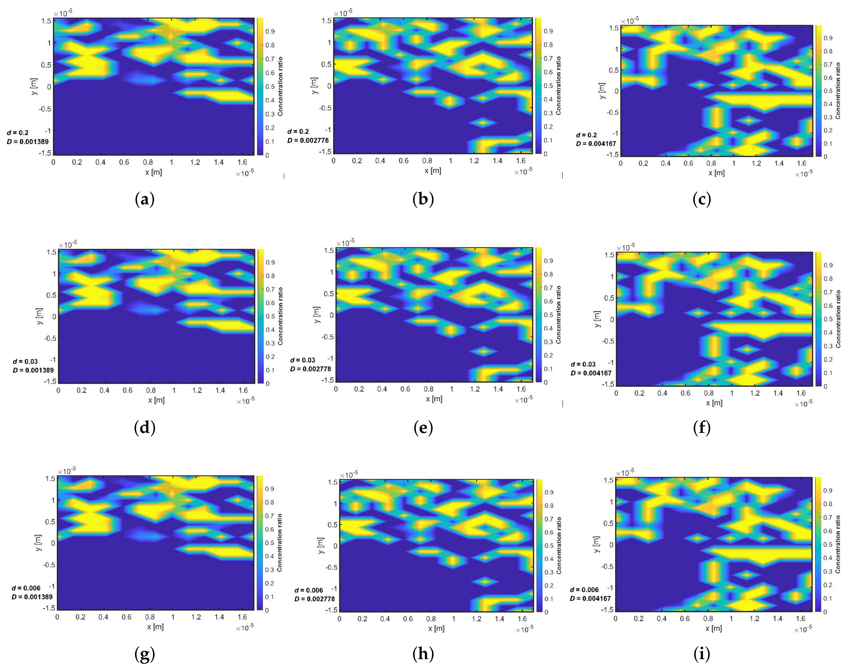
  • Variation of dispersion coefficients from the solution was found to affect the concentration distribution even at low Reynolds number region.
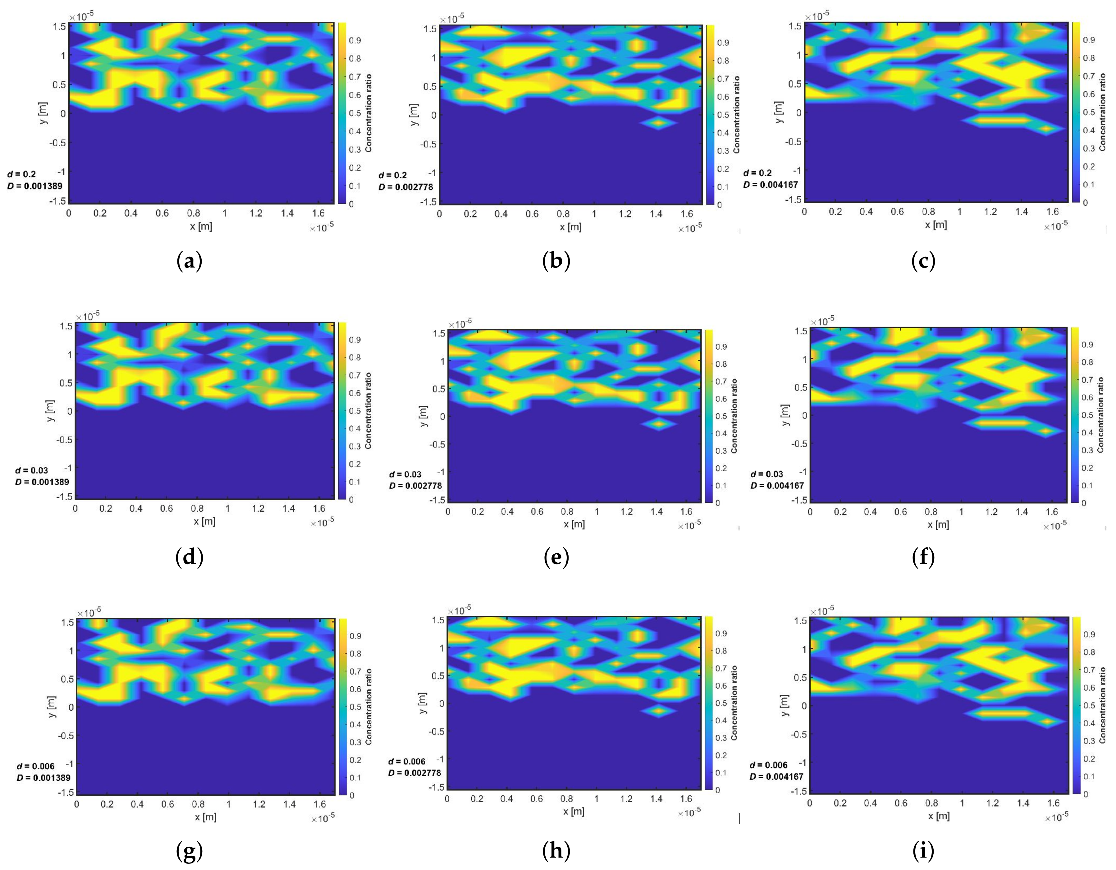
  • Linear drift effect at low creeping flow regime was found to affect tracer concentration distribution at a later time.
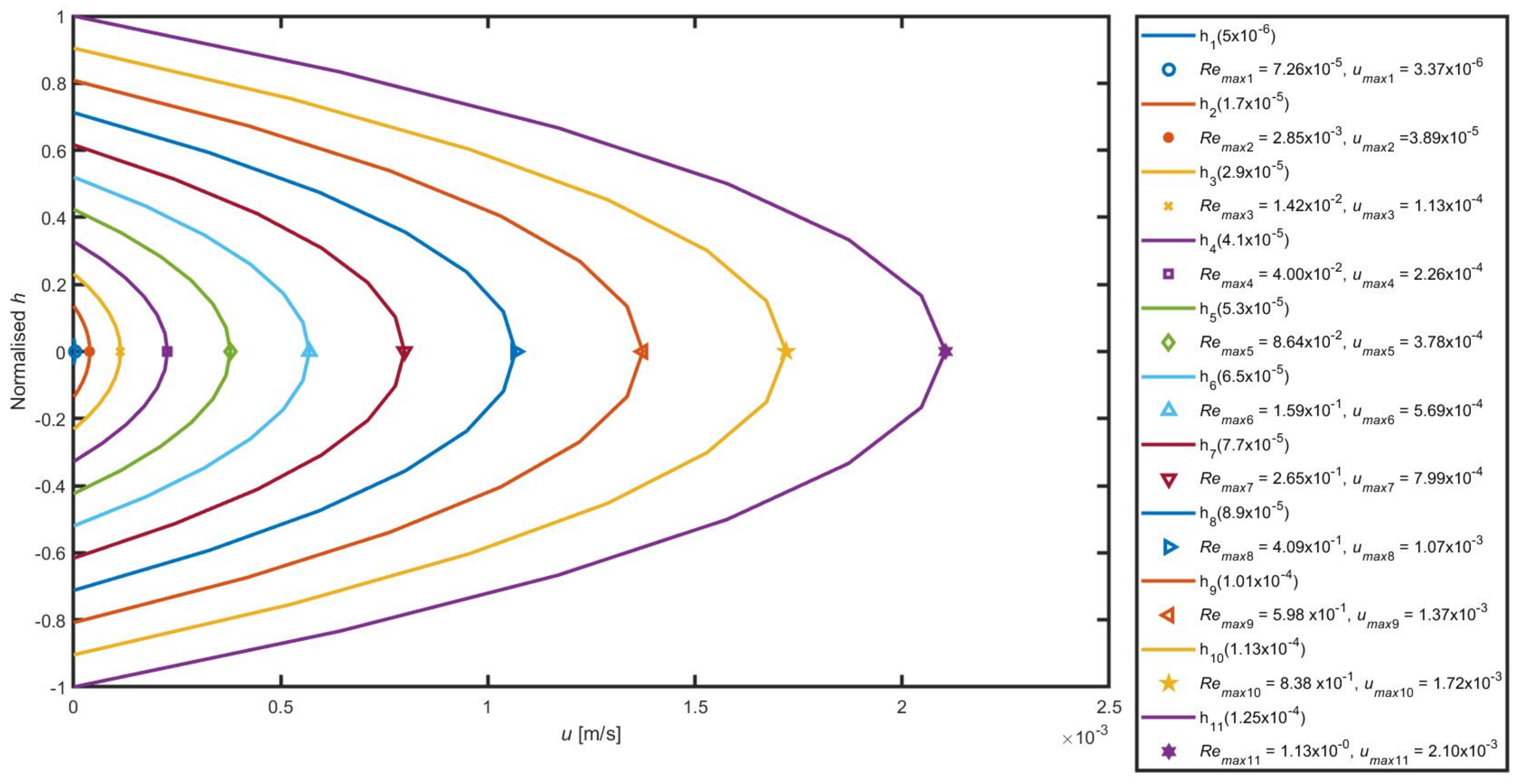
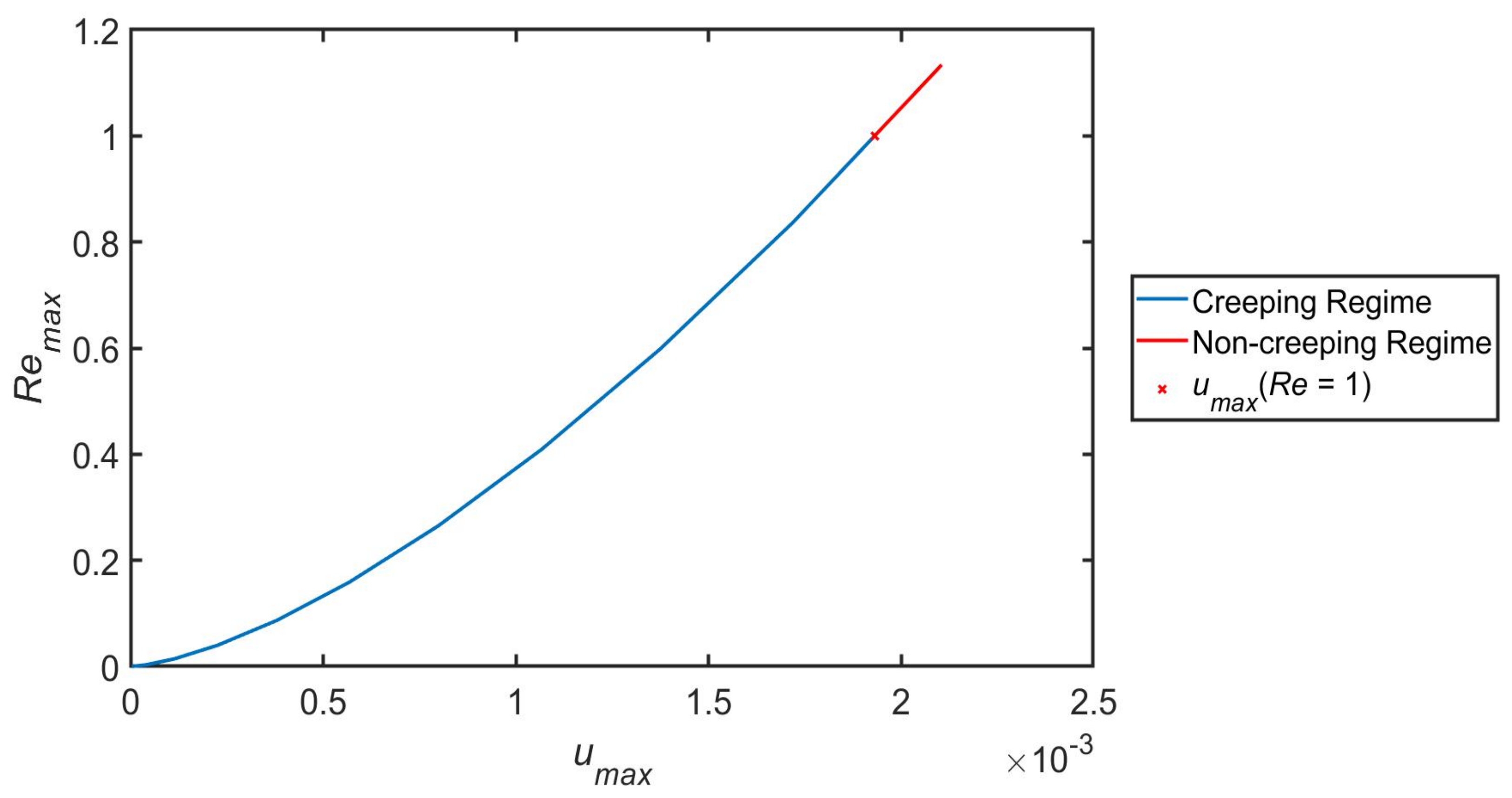
  • Stokes flow approximation has been invoked and consequently the analysis of the results is valid in the limits of small Reynolds numbers of <1. However, the behaviour of the flow is likely to change for higher values of Reynolds number. The drift effect is then evaluated at a creeping flow regime. An increase in the flow velocity at the centre of the channel/porous media is noticed in all the cases from a creeping flow regime to a non-creeping flow regime.
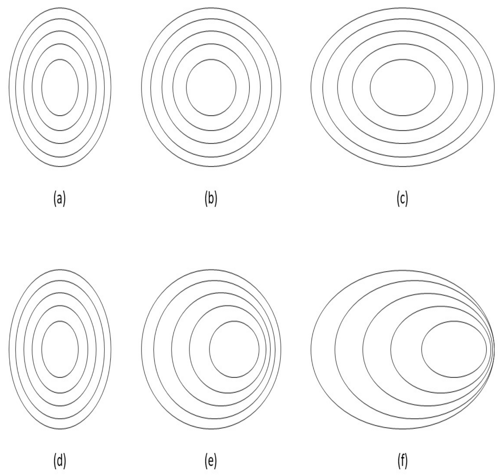
  • The influence of linear drift on the concentration profile was evaluated in all the directions for a system with non-homogeneous porosity distribution and variable velocity profiles. Analysis of the results shows that the effect of linear drift on concentration profile depends on system heterogeneity and increases at later times.
  • Flow velocities and concentration distribution data sets collected in this study proved to be essential and valuable for the development and testing of pore-scale numerical transport model under the influence of drift.
  • This study can be used to identify the main transport path of tracers during enhanced oil recovery studies in porous media.

Author Contributions

Conceptualisation, I.A., L.T.A., J.L.G. and G.K.F.; investigation, I.A., L.T.A., J.L.G. and G.K.F.; writing—original draft, I.A. All authors have read and agreed to the published version of the manuscript.

Funding

Petroleum Technology Development Fund—PTDF (Nigeria).

Institutional Review Board Statement

Not applicable.

Informed Consent Statement

Not applicable.

Data Availability Statement

Not applicable.

Acknowledgments

We express our appreciation to the Petroleum Technology Development Fund, Nigeria (PTDF), for funding this research project.

Conflicts of Interest

The authors declare no conflict of interest.

Nomenclature

k r Chemical reaction constant, d 1
sLaplace transform parameter
Γ x Gamma function
k , μ Whittaker and Kummer functions parameters
iUnit vector along the x-axis
Ψ Concentration function
jUnit vector along the y-axis
kUnit vector along the z-axis
LLength of dispersion, (m)
QInjection rate, m 3 / s
W k , μ ξ Whittaker function with parameter k , μ
M k , μ ξ Whittaker function with parameter k , μ
U a , b , z Tricomi Kummer U-function with parameters (a,b,z)
ω 2 Absolute value of separation constant
ϕ Porosity, dimensionless
θ Angle,
CTracer concentration
DFlow hydrodynamic dispersion m 2 / s
dDrift ratio
D m Molecular diffusion constant
D o Shear mixing constant
hChannel thickness, in Nano-metre ( n m )
td
S m saturation of the mobile fluid phase
uPoiseuille velocity ( m / s )
rRadial distance from the pore, (m)
ΦChromatographic response function
γRetardation constant

Appendix A. Derivation of the Analytical Solution to the Navier–Stokes Equation

ρ v t + ρ v · ( v ) = p + μ 2 v
Applying the following assumptions:
  • Steady state, the transient acceleration term i.e ρ v t = 0
  • Unidirectional, pressure gradient is only in the X-direction and the plates are motionless.
  • Velocity vector and the velocity gradient tensor are off-diagonal; therefore, the dot product is zero. Hence Equation (A1) reduces to:
d p d x = μ 2 v y 2
From Equation (A2), d p d x , means the pressure gradient is only in the x-direction and is uniform. i.e., it is constant. Also μ 2 v y 2 means there is a velocity vector that only has an x-component and gradient in the y-direction. Integrating Equation (A2) with respect to y we obtain:
1 2 μ d p d x y 2 = v + c 1 y + c
v = 1 2 μ d p d x y 2 c 1 y c 2
Applying the following boundary conditions:and y = h , v = 0 . From the first boundary conditions, c 2 = 0 . From Equation (A4). therefore Equation (A4) reduces to:
v = 1 2 μ d p d x y 2 c 1 y
Applying the second boundary condition, Equation (A5) becomes:
0 = 1 2 μ d p d x y 2 c 1 y
Therefore:
c 1 = 1 2 μ d p d x h
Substitute for c 1 and c 2 into Equation (A4) to obtain:
v = 1 2 μ d p d x h y y

Appendix B. Derivation of the Transport Flow Equation with Linear Drift

The Transport Equation (2) can be expanded by considering a steady-state condition thus:
1 r D d C d r + r D d C d r + r D d 2 C d r 2 1 r { v C + r v C + r v d C d r } γ ϕ k r + s C = 0
But γ ϕ = Φ is the chromatographic response function which measures the quality of separation of tracers from solvent during flow and transport.
d 2 C d r 2 + D v D + 1 r d C d r r v + v D r + Φ k r + s D C = 0
where all variables are defined in the main text. Let:
C = ψ e x p 1 2 D v D + 1 r d r
Then:
d C d r = d ψ d r . e 1 2 D v D + 1 r 1 2 D v D + 1 r ψ e 1 2 D v D + 1 r
and:
d 2 C d r 2 = d d r { d ψ d r . e 1 2 D v D + 1 r 1 2 D v D + 1 r ψ e 1 2 D v D + 1 r }
= d 2 ψ d r 2 . e 1 2 D v D + 1 r 1 2 D v D + 1 r d ψ d r . e 1 2 D v D + 1 r 1 2 D v D + 1 r ψ . e 1 2 D v D + 1 r 1 2 D v D + 1 r d ψ d r . e 1 2 D v D + 1 r + 1 4 D v D + 1 r 2 ψ e 1 2 D v D + 1 r
d 2 C d r 2 = d 2 ψ d r 2 D v D + 1 r d ψ d r 1 2 D v D + 1 r 1 4 D v D + 1 r 2 ψ e 1 2 D v D + 1 r
Let:
d 2 C d r 2 + D v D + 1 r = I
With the first order differential component d C d r defined by Equation (A12), then:
I = d 2 ψ d r 2 . e 1 2 D v D + 1 r D v D + 1 r d ψ d r . e 1 2 D v D + 1 r 1 2 D v D + 1 r 1 4 D v D + 1 r 2 ψ e 1 2 D v D + 1 r + D v D + 1 r e 1 2 D v D + 1 r d ψ d r 1 2 D v D + 1 r ψ e 1 2 D v D + 1 r
Substituting Equations (A11) and (A17) in (A9) and rearranging gives:
d 2 ψ d r 2 { 1 2 D v D + 1 r + D v D + 1 r 2 + r v + v D r + Φ k r + s D } ψ = 0
Expressing the effective fluid velocity v in dimensionless form:
p 2 μ h y y 2 = v d + α r
D r = k + β p r
= k + β p r 1
D r = β p r 2 = β p r 2
Thus:
D r v = β p r 2 p 2 μ h y y 2
D v D r = β p r r 2 k r + β p p 2 μ h y y 2 r k r + β p
= β p r k r + β p p h y y 2 r 2 μ k r + β p
Let:
I β p r k r + β p = A r + B k r + β p
then:
β p = A k r + β p + B r
r = 0 β p = A β p + 0 A = 1
B = β p + k + β p = k
so that:
I β p r k r + β p = k k r + β p 1 r
Therefore:
D r v D r = k k r + β p 1 r p h y y 2 r 2 μ k r + β p
D r v D r + 1 r = k k r + β p p h y y 2 r 2 μ k r + β p
D r v D r + 1 r = k 2 k r + β p 2 p h y y 2 2 μ k r + β p + p k h y y 2 r 2 μ k r + β p 2
= p k h y y 2 r 2 μ k 2 2 μ k r + β p 2 p h y y 2 2 μ k r + β p
r v + v D r = 0 + p 2 μ h y y 2 k r + β p
= p h y y 2 2 μ k r + β p
Therefore, Equation (A18) becomes:
d 2 ψ d r 2 { 1 2 p k h y y 2 r 2 μ k 2 2 μ k r + β p 2 p h y y 2 2 μ k r + β p + 1 4 k k r + β p p h y y 2 2 μ k r + β p 2 + p h y y 2 2 μ k r + β p + Φ k r + s k r + β p } ψ = 0
d 2 ψ d r 2 p k h y y 2 r 2 μ k 2 4 μ k r + β p 2 p h y y 2 2 μ k r + β p ψ k 2 k r + β p + p 2 h y y 2 2 r 2 16 μ 2 k r + β p 2 + k p h y y 2 r 4 μ k r + β p 2 ψ p h y y 2 + 2 μ Φ k r + s r 2 μ k r + β p ψ = 0
= d 2 ψ d r 2 p k h y y 2 r 4 μ k r + β p 2 ψ + k 2 2 k r + β p 2 ψ + p h y y 2 2 μ k r + β p ψ k 2 4 k r + β p 2 ψ p 2 h y y 2 2 r 2 16 μ 2 k r + β p 2 ψ + p k h y y 2 r 4 μ k r + β p 2 ψ p h y y 2 2 μ k r + β p ψ Φ k r + s k r + β p ψ = 0
An expression of the form:
d 2 ψ d r 2 + 1 4 k 2 k r + β p 2 p 2 h y y 2 r 2 16 μ 2 k r + β p 2 Φ k r + s r k r + β p ψ = 0
is therefore obtained for the general pore-scale convection–diffusion equation in Laplace space. And it can be written in dimensionless form as:
d 2 ψ d r D 2 + [ 1 4 k 2 k r D + β p 2 p 2 h y y 2 2 r D 2 16 μ 2 k r D + β p 2 Φ k r + s r D k r D + β p ] ψ = 0
Recall that:
η = k r D + β
r D = η β 1 k d r D d η = 1 k
d r D d η = k d r D = 1 k η
d 2 ψ d r D 2 = d d r D d ψ d r D = d 1 k d η d ψ 1 k d η = 1 1 k 2 d d η d ψ d η = k 2 d 2 ψ d η 2
k 2 d 2 ψ d η 2 + { [ 1 4 k 2 η 2 p 2 h y y 2 2 η β 2 1 k 2 16 μ 2 η 2 Φ k r + s η β 1 k η ] } ψ = 0
= k 2 d 2 ψ d η 2 + { k 2 4 η 2 p 2 h y y 2 η β 2 16 μ 2 k 2 η 2 ϕ k r + s k + Φ k r + s β k η } ψ = 0

Appendix C. Transformation and Simplification of Pore-Scale Convection–Diffusion Equation to the General Whittaker Equation

However, applying the transformation of Section 3 to Equation (4) gives:
k 2 d 2 ψ d η 2 + { k 2 4 η 2 p 2 h y y 2 2 η β 1 k 2 16 μ 2 η 2 Φ k r + s η β 1 k η } ψ = 0
Simplifying Equation (A48) above:
k 2 d 2 ψ d η 2 + { k 2 4 η 2 p 2 h y y 2 η 2 2 η β + β 2 16 μ 2 k 2 η 2 Φ k r + s k η η β } ψ = 0
= k 2 d 2 ψ d η 2 + { k 2 4 η 2 p 2 ( h y y 2 ) 16 μ 2 k 2 ( 1 2 β η + β 2 η 2 ) Φ ( k r + s ) k 1 β η } ψ = 0
d 2 ψ d η 2 + { 1 4 η 2 p 2 h y y 2 16 μ 2 k 4 1 2 β η + β 2 η 2 Φ k r + s k 3 1 β η } ψ = 0
Further, simplification of Equation (A52) gives:
d 2 ψ d η 2 + 1 4 p 2 β 2 h y y 2 16 μ 2 k 4 1 η 2 + p 2 h y y 2 β 8 μ 2 k 4 + β ϕ k r + s 1 η ψ p 2 h y y 2 16 μ 2 k 2 + Φ k r + s k 1 k 2 ψ = 0
Equation (A53) can be written in the form of Whittaker equation by changing some variables defined as:
ξ = 2 η a
where:
a = 1 k 2 p 2 h y y 2 16 μ 2 k 2 + Φ k r + s k
= f s 2
Then:
d s d η = 2 f s d s = 2 f s d η d s d f s = d η
d ψ d η = d ψ d s . d s d η = 2 f s d ψ d s
and
d 2 ψ d η 2 = d d η d ψ d η = d d ξ 2 f s d ψ d ξ 2 f s
= 1 1 4 f s 2 d 2 ψ d ξ 2
Substituting Equations (A58) and (A60) into Equation (A53) gives:
4 f s 2 d 2 ψ d ξ 2 + { 1 4 p 2 β 2 h y y 2 16 μ 2 k 4 4 f s 2 ξ 2 + p 2 h y y 2 β 8 μ 2 k 4 + β Φ k r + s 2 f s ξ f s 2 } ψ = 0
d 2 ψ d ξ 2 + { 1 4 p 2 β 2 h y y 2 16 μ 2 k 4 1 ξ 2 + p 2 h y y 2 β 8 μ 2 k 4 + β Φ k r + s 1 2 f s ξ 1 4 } ψ = 0
Hence Equation (A62) can now be written as:
d 2 ψ d ξ 2 + { 1 4 p 2 β 2 h y y 2 16 μ 2 k 4 1 ξ 2 + p 2 h y y 2 β 16 μ 2 k 4 f s + β Φ k r + s 2 f s 1 ξ 1 4 } ψ = 0
Equation (A63) is the equation that is written in the form of Whittaker Equation (8) in Section 3 of the main text.

Appendix D. Analytical Solution of Tracer Concentration and Its Weak-Form Solution

Detailed solution of the general whittaker equation can be found in Akanji and Falade [16]. Tracer concentration can now be written as:
C η r , s = ψ e 1 2 k k r + β w p h y y 2 2 μ r k r + β w d r
The solution to Equations (A62)–(A64) can therefore be expressed as:
ψ ξ = e ξ 2 ξ 1 2 + μ U 1 2 + μ k , 1 + 2 μ , ξ
However, the concentration C is defined in terms of ψ as:
C = ψ e 1 2 D v D + 1 r D d r D
or:
C = ψ e 1 2 k k r D + β w p h y y 2 r D 2 μ k r D + β w d r D
C = ψ k r D + β 1 2 p h y y 2 β 4 μ k 2 e p h y y 2 4 μ k 2
C = k r D + β 1 2 p h y y 2 β 4 μ k 2 e p h y y 2 4 μ k 2 e ξ 2 ξ 1 2 + μ U 1 2 + μ k , 1 + 2 μ , ξ
so that:
C = η 1 2 p h y y 2 β 4 μ k 2 e p h y y 2 4 μ 2 k e η a 2 η a 1 2 + μ U 1 2 + μ k , 1 + 2 μ , ξ
C = η 1 2 p h y y 2 4 μ k 2 + 1 2 + μ 2 η a 1 2 + μ e p h y y 2 4 μ 2 k η a U 1 2 + μ k , 1 + 2 μ , ξ
C = η μ p h y y 2 4 μ 2 k 2 η a 1 2 + μ e p h y y 2 4 μ 2 k η a U 1 2 + μ k , 1 + 2 μ , 2 η a
or:
C = ξ 2 a 1 2 p h y y 2 β 4 μ k 2 e p h y y 2 4 μ 2 k e ξ 2 ξ 1 2 + μ U 1 2 + μ k , 1 + 2 μ , ξ
C = ξ 1 2 p h y y 2 β 4 μ k 2 + 1 2 + μ 2 a 1 2 + p h y y 2 β 4 μ k 2 e p h y y 2 4 μ 2 k ξ 2 U 1 2 + μ k , 1 + 2 μ , ξ
C = ξ μ p h y y 2 4 μ k 2 2 a 1 2 + p h y y 2 β 4 μ k 2 e p h y y 2 4 μ 2 k ξ 2 U 1 2 + μ k , 1 + 2 μ , ξ
where a is given as:
a = 1 k 2 p 2 h y y 2 16 μ 2 k 2 + Φ k r + s k
= 1 16 μ 2 k 4 p 2 h y y 2 + 16 μ 2 k Φ k r + s
and:
ξ = 2 a η
ξ = 2 a k r D + β
ξ = 1 2 μ k 2 p 2 h y y 2 + 16 μ 2 k Φ k r + s k r D + β
ξ r D = 1 2 μ k 2 p 2 h y y 2 + 16 μ 2 k Φ k r + s k r + β
Having developed the transport equation for flow of tracers at pore scale, the weak-form solution of Equation (17) is now presented in Laplace space by adopting the separation of variables with X-parameter (Xp) and Y-parameter (Yp), thus:
C x , y , s = X p x Y p y , s
The X-parameter (Xp) can be expressed as:
X p x = τ U 1 2 + μ k , 1 + 2 μ , σ ξ X p e 1 2 1 σ 1 ξ X p
where the components and arguments of the Tricomi Kummer function U (a, b, x) are defined thus:
ξ X p = β p 2 μ h y y 2 D o d + p 2 μ h y y 2 D o x
σ = 1 4 ω 2 D o p 2 μ h y y 2 d
h = ω 2 β p 2 μ h y y 2 d 2
and Y-parameter (Yp):
Y p y , s = 1 3 ξ Y p 1 2 + μ e p 2 μ h y y 2 y 2 D o I 1 3 2 3 L ξ Y p 3 2 + μ + I + 1 3 2 3 L ξ Y P 3 2 + μ
ξ Y p = 1 4 p 2 μ h y y 2 D o 2 + R s + R k + ω 2 D o λ Y
I is modified Bessel functions of the first kind and decays to zero rapidly with the concentration distribution of the Y (y,s) component in the negative half, depicting the positive half.

Appendix E. Analytical Solution—Dimensionless Representation and Inverse Laplace Transform

In dimensionless radial length r D , C η r , s can be written as:
C η r , s = ψ 1 2 k k r D + β p h y y 2 r D 2 μ k r D + β d r D
= ψ e 1 2 k η p h y y 2 2 μ η η β k d η k
= ψ e 1 2 1 η + p h y y 2 β 2 μ k 2 η p h y y 2 2 μ k 2 d η
= ψ e 1 2 1 + p h y y 2 2 μ k 2 l n η p h y y 2 η 2 μ k 2
= ψ e l n η 1 2 1 + p h y y 2 2 μ k 2 . e p h y y 2 4 μ k 2 η
ψ ξ , s = e 1 2 ξ 1 2 + μ U 1 2 + μ k , 1 + 2 μ , ξ
A s = 2 1 2 1 + p h y y 2 2 μ k 2 ξ 1 2 1 + p h y y 2 2 μ k 2 1 2 μ f s 1 2 1 + p h y y 2 2 μ k 2
ξ = 2 η f s η = ξ 2 f s
therefore:
C ξ , s = ψ 2 f s 1 2 1 + p h y y 2 2 μ k 2 e p h y y 2 4 μ k 2 ξ 2 f s
C ξ , s = ψ ξ 1 2 1 + p h y y 2 2 μ k 2 2 1 2 1 + p h y y 2 2 μ k 2 f s 1 2 1 + p h y y 2 2 μ k 2 e p h y y 2 8 μ k 2 ξ f s
ψ = C ξ , s ξ 1 2 1 + p h y y 2 2 μ k 2 2 1 2 1 + p h y y 2 2 μ k 2 f s 1 2 1 + p h y y 2 2 μ k 2 e p h y y 2 8 μ k 2 ξ f s
= B s e ξ 2 ξ 1 2 + μ U 1 2 + μ k , 1 + 2 μ , ξ
B s = C ξ , s ξ 1 2 1 + p h y y 2 2 μ k 2 2 1 2 1 + p h y y 2 2 μ k 2 f s 1 2 1 + p h y y 2 2 μ k 2 e p h y y 2 8 μ k 2 ξ f s e ξ 2 ξ 1 2 + μ U 1 2 + μ k , 1 + 2 μ , ξ
Let: U 1 2 + μ k , 1 + 2 μ , ξ = R
B s = C ξ , s 2 1 2 1 + p h y y 2 2 μ k 2 ξ 1 2 1 + p h y y 2 2 μ k 2 + 1 2 + μ f s 1 2 1 + p h y y 2 2 μ k 2 e p h y y 2 8 μ k 2 ξ f s ξ 2 R
B s = C ξ , s 2 1 2 1 + p h y y 2 2 μ k 2 ξ μ p h y y 2 2 μ k 2 f s 1 2 1 + p h y y 2 2 μ k 2 e ξ 2 1 p h y y 2 4 μ k 2 ξ f s R
Now:
C ξ , s = ψ ξ 1 2 1 + p h y y 2 2 μ k 2 2 1 2 1 + p h y y 2 2 μ k 2 f s 1 2 1 + p h y y 2 2 μ k 2 e p h y y 2 8 μ k 2 ξ f s
C ξ , s = e ξ 2 ξ 1 2 + μ U 1 2 + μ k , 1 + 2 μ , ξ ξ 1 2 1 + p h y y 2 2 μ k 2 2 1 2 1 + p h y y 2 2 μ k 2 f s 1 2 1 + p h y y 2 2 μ k 2 e p h y y 2 8 μ k 2 ξ f s
C ξ , s = 2 1 2 1 + p h y y 2 2 μ k 2 ξ μ p h y y 2 4 μ k 2 f s 1 2 1 + p h y y 2 2 μ k 2 e p h y y 2 4 μ k 2 1 f s ξ 2 R
d C ξ , s d ξ = μ p h y y 2 4 μ k 2 2 1 2 1 + p h y y 2 2 μ k 2 ξ μ p h y y 2 4 μ k 2 f s 1 2 1 + p h y y 2 4 μ k 2 e p h y y 2 4 μ k 2 f s 1 ξ 2 R + p h y y 2 8 μ k 2 f s 1 2 2 1 2 1 + p h y y 2 2 μ k 2 ξ μ p h y y 2 4 μ k 2 f s 1 2 1 + p h y y 2 4 μ k 2 e p h y y 2 4 μ k 2 f s 1 ξ 2 R 1 2 + μ k 2 1 2 1 + p h y y 2 2 μ k 2 ξ μ p h y y 2 4 μ k 2 f s 1 2 1 + p h y y 2 4 μ k 2 e p h y y 2 4 μ k 2 f s 1 ξ 2 R
However, U 1 2 + μ k , 1 + 2 μ , ξ = R is used from Equations (A102)–(A107) to avoid equation breakthrough.
= 2 1 2 1 + p h y y 2 2 μ k 2 ξ μ p h y y 2 4 μ k 2 f s 1 2 1 + p h y y 2 4 μ k 2 e p h y y 2 4 μ k 2 f s 1 ξ 2 U 1 2 + μ k , 1 + 2 μ , ξ μ p h y y 2 4 μ k 2 ξ 1 + p h y y 2 8 μ k 2 f s 1 2 1 2 + μ k U 1 2 + μ k , 1 + 2 μ , ξ U 1 2 + μ k , 1 + 2 μ , ξ
d C ξ , s d ξ = { μ ξ 1 p h y y 2 4 μ k 2 ξ 1 + p h y y 2 8 μ k 2 f s 1 2 1 2 + μ k U 1 2 + μ k , 1 + 2 μ , ξ U 1 2 + μ k , 1 + 2 μ , ξ } C ξ , s
However:
η = k r D + β ξ 2 f s = k r D + β
d s 2 f s = k d r D d s = 2 k f s d r D
Thus:
d C ξ , s 2 k f s d r D = { 1 ξ μ p h y y 2 4 μ k 2 1 2 1 p h y y 2 8 μ k 2 f s 1 2 + μ k U 1 2 + μ k , 1 + 2 μ , ξ U 1 2 + μ k , 1 + 2 μ , ξ } C ξ , s
d C ξ , s d r D = { 1 ξ μ p h y y 2 4 μ k 2 1 2 1 p h y y 2 8 μ k 2 f s 1 2 + μ k U 1 2 + μ k , 1 + 2 μ , ξ U 1 2 + μ k , 1 + 2 μ , ξ } C ξ , s
but:
U 1 2 + μ k , 1 + 2 μ , ξ U 1 2 + μ k , 1 + 2 μ , ξ = 1 ξ = 1 2 η f s
d C ξ , s d r D = 2 k f s { 1 ξ μ p h y y 2 4 μ k 2 1 2 1 p h y y 2 8 μ k 2 f s 1 2 + μ k 1 ξ } C ξ , s
1 f s d C ξ , s d r D = 2 k { 1 ξ μ p h y y 2 4 μ k 2 1 2 1 p h y y 2 8 μ k 2 f s 1 2 + μ k 1 ξ } C ξ , s
1 f s d C ξ , s d r D = 2 k { 1 ξ k 1 2 p h y y 2 4 μ k 2 1 2 + p h y y 2 16 μ k 2 f s } C ξ , s
1 f s d C ξ , s d r D = k { 1 ξ 2 k 1 p h y y 2 2 μ k 2 1 + p h y y 2 8 μ k 2 f s } C ξ , s
1 f s d C ξ , s d r D = k { 1 η f s k 1 2 p h y y 2 4 μ k 2 1 + p h y y 2 8 μ k 2 f s } C ξ , s
However:
k = p 2 β h y y 2 16 μ k 4 f s + β Φ k r + s 2 f s
Therefore:
1 f s d C ξ , s d η = { 1 2 η f s [ p 2 β h y y 2 16 μ k 4 f s + β Φ k r + s 2 f s 1 2 p h y y 2 4 μ k 2 ] 1 2 + p h y y 2 16 μ k 2 f s } C ξ , s
1 f s d C ξ , s d η = 1 2 C ξ , s + { p h y y 2 16 μ k 2 1 4 η p h y y 2 8 μ η k 2 f s + p 2 β h y y 2 32 η μ 2 k 4 + β Φ k r + s 4 η f s 2 } C ξ , s
1 2 C ξ , s = 1 f s d C ξ , s d η + { p h y y 2 16 μ k 2 1 4 η p h y y 2 8 μ η k 2 f s + p 2 β h y y 2 32 η μ 2 k 4 + β Φ k r + s 4 η f s 2 } C ξ , s
1 2 k C ξ , s = 1 k f s d C ξ , s d η { p h y y 2 16 μ k 2 1 4 η p h y y 2 8 μ η k 2 k f s + p 2 β h y y 2 32 η μ 2 k 3 + k β Φ k r + s 4 η k 2 f s 2 } C ξ , s
but:
k f s = k a = k . 1 k p 2 h y y 2 16 μ 2 k 2 + Φ k r + s k
= p 2 h y y 2 16 μ 2 k 2 + Φ k r + s k
k f s = φ k p 2 h y y 2 16 μ φ k + k r + s
The inverse Laplace transform of s 1 is:
L 1 1 φ k p 2 h y y 2 16 μ φ k + k r + s = e p 2 h y y 2 16 μ 2 φ k + k r t φ k π t
Similarly, the inverse Laplace transform of f ( s ) 2 is:
L 1 1 φ k p 2 h y y 2 16 μ φ k + k r + s 2 = e p 2 h y y 2 16 μ 2 φ k + k r t φ k
Evaluating the inverse Laplace transform of the general solution as:
1 2 k C ξ , s = k φ 0 t d C ξ , τ d η e p 2 h y y 2 16 μ 2 φ k + k r t τ π t τ d τ k φ p h y y 2 16 μ k 4 1 4 η p h y y 2 8 μ η k 2 0 t C ξ , τ e p 2 h y y 2 16 μ 2 φ k + k r t τ π t τ d τ p 2 β h y y 2 32 η μ 2 φ k 2 + k 2 β ϕ k r + s 4 φ η 0 t C ξ , τ e p 2 h y y 2 16 μ 2 φ k + k r t τ d τ
f s = 1 k p 2 h y y 2 16 μ 2 k 2 + Φ k r + s k
f s = 1 D m + β w p 2 h y y 2 16 μ 2 D m + β w 2 + Φ k r + s D m + β w
Equations (10) and (11) becomes:
μ = p β h y y 2 4 μ k 2
p v p D o h y y 2 4 μ D m + D o v d 2 = p v p D o h y y 2 4 μ D m 2 1 + D o v d D m 2
k = p 2 β h y y 2 16 μ 2 k 4 f s + β Φ k r + s 2 f s
= p 2 v p D o h y y 2 16 μ 2 D m + D o v d 4 f s + v w D o Φ k r + s 2 f s
= p 2 v p D o h y y 2 16 μ 2 D m 1 + D o v d D m 4 f s + v w D o Φ k r + s 2 f s

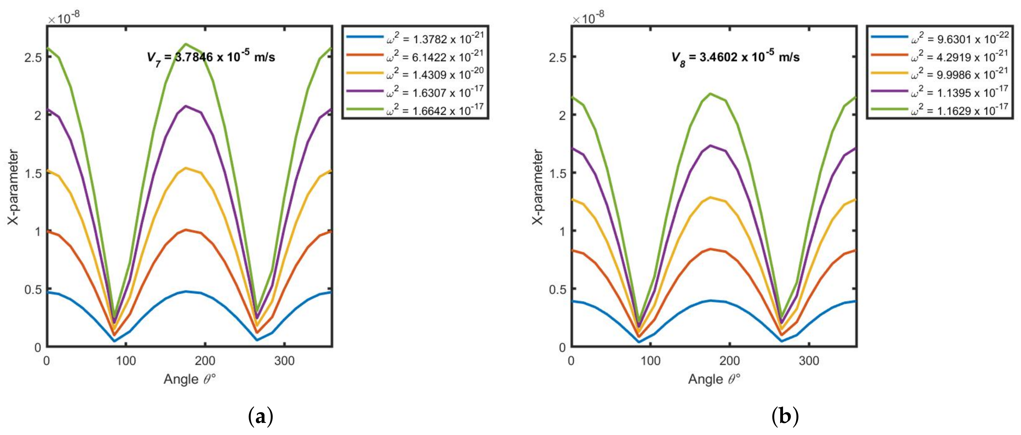
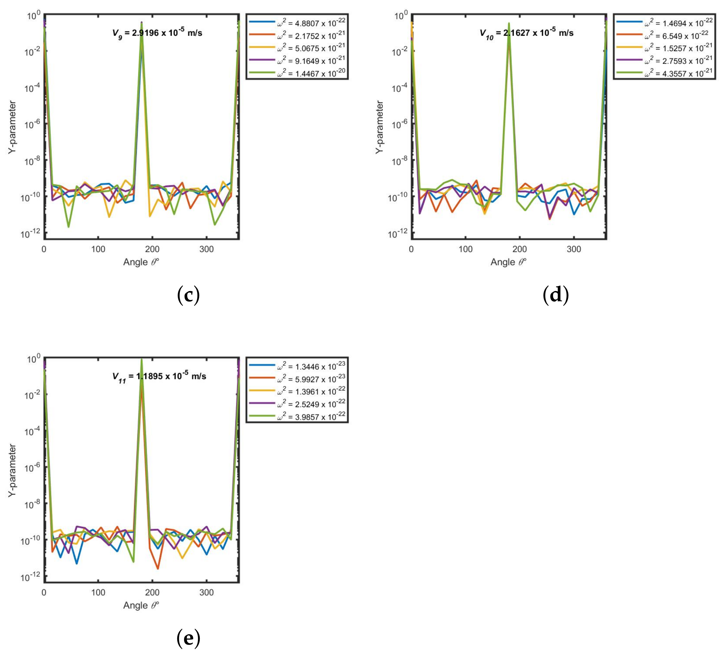
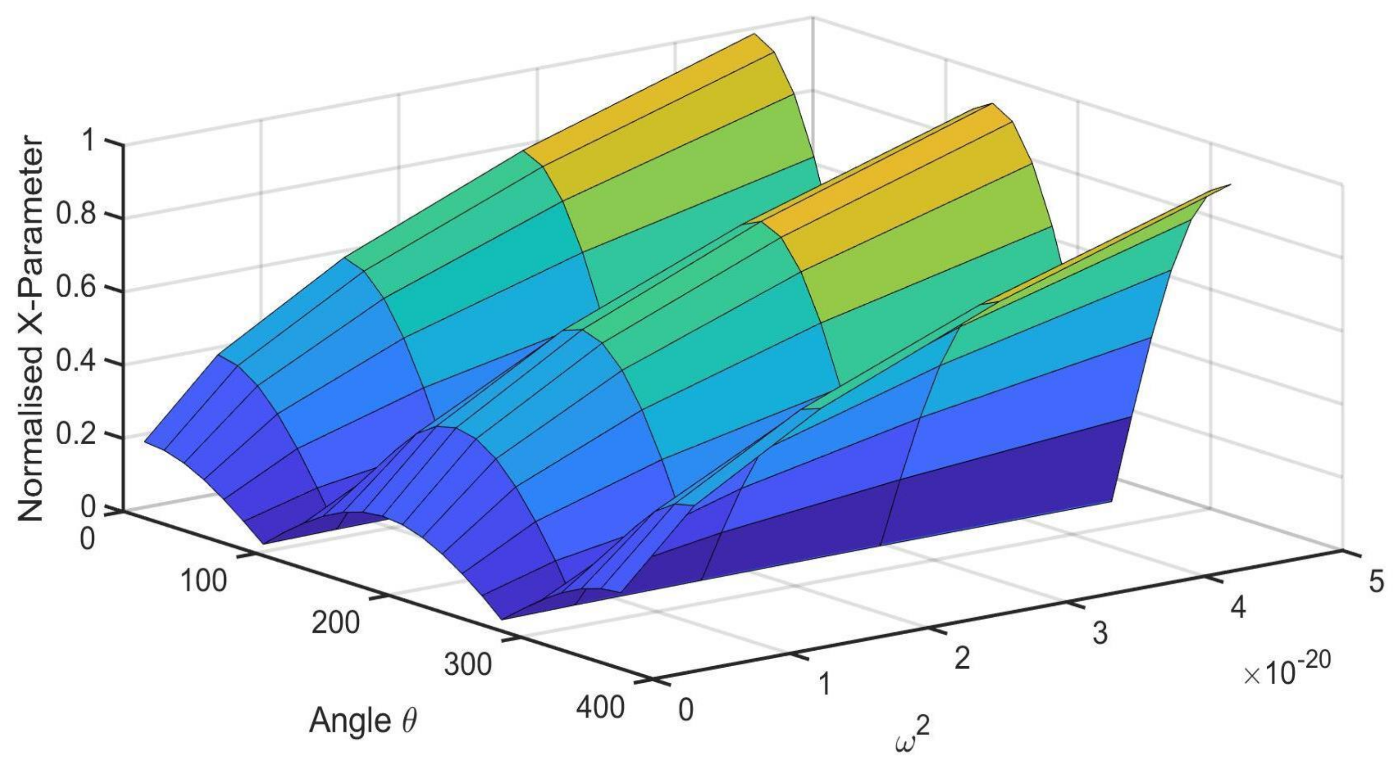
Appendix F. Symmetrical X-Parameter(Xp) and Y-Parameter (Yp) as a Function of Angle (θ) at a Thickness of h = 1.7 × 10⁻⁵ m, time t = 10 Days and Varying Separation Constant (ω2)

Figure A1. X-parameter ( X p ) as a function of angle ( θ ) for channel thickness h = 1.7 × 10 5 m, time t = 10 d and varying separation constant ( ω 2 ) . These results correspond to the second half-wing of those presented in Figure 5. (a) v 7 = 3.7846 × 10 5 m/s, (b) v 8 = 3.4602 × 10 5 m/s (c) v 9 = 2.9196 × 10 5 m/s (d) v 10 = 2.1627 × 10 5 m/s and (e) v 11 = 1.1895 × 10 5 m/s.
Mathematics 09 02509 g0a1aMathematics 09 02509 g0a1b
Figure A2. Y- p a r a m e t e r (Y p ) as a function of angle ( θ ) for channel thickness h = 1.7 × 10 5 m, time t = 10 d and varying separation constant ( ω 2 ) . These results correspond to the second half-wing of those presented in Figure 6. (a) v 7 = 3.7846 × 10 5 m/s, (b) v 8 = 3.4602 × 10 5 m/s (c) v 9 = 2.9196 × 10 5 m/s (d) v 10 = 2.1627 × 10 5 m/s and (e) v 11 = 1.1895 × 10 5 m/s.
Mathematics 09 02509 g0a2aMathematics 09 02509 g0a2b

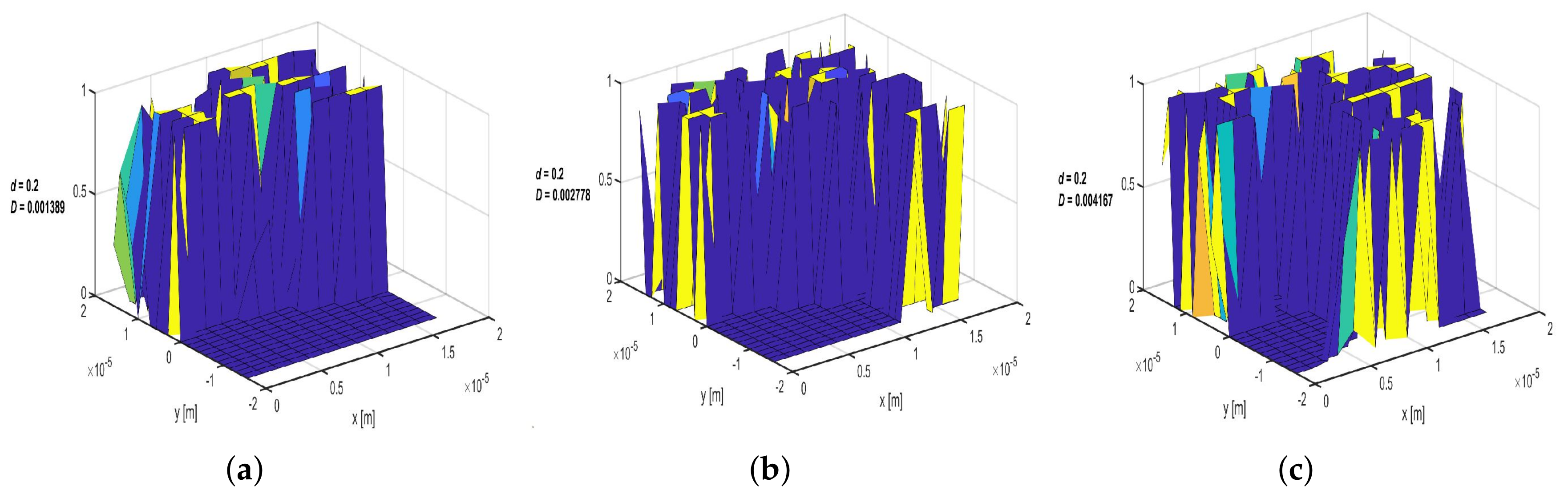
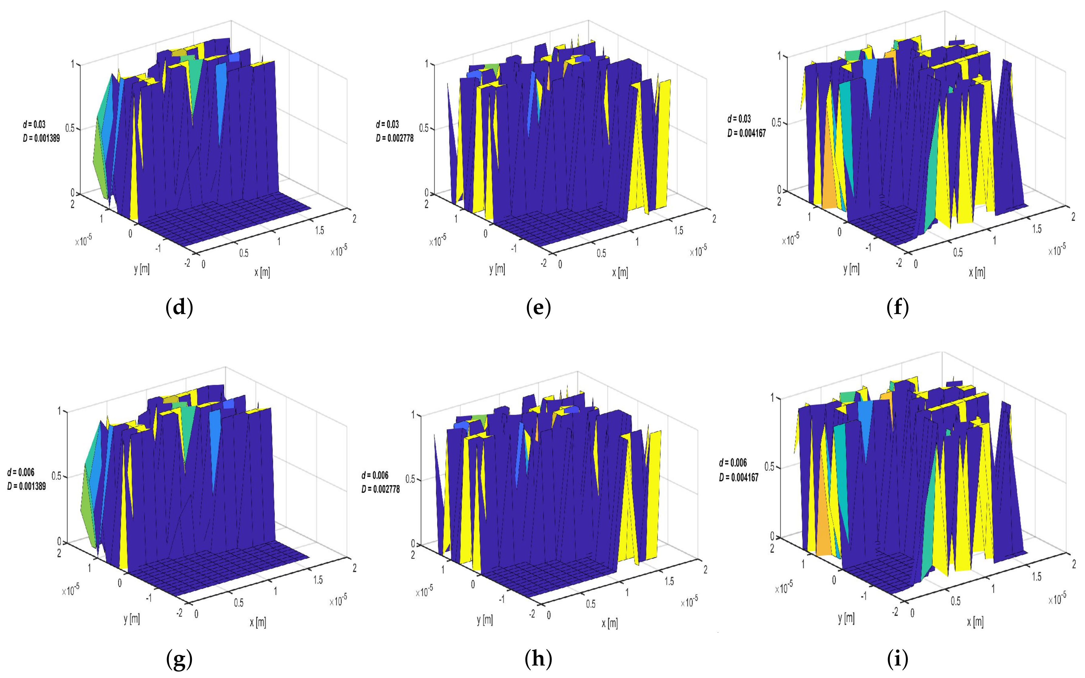
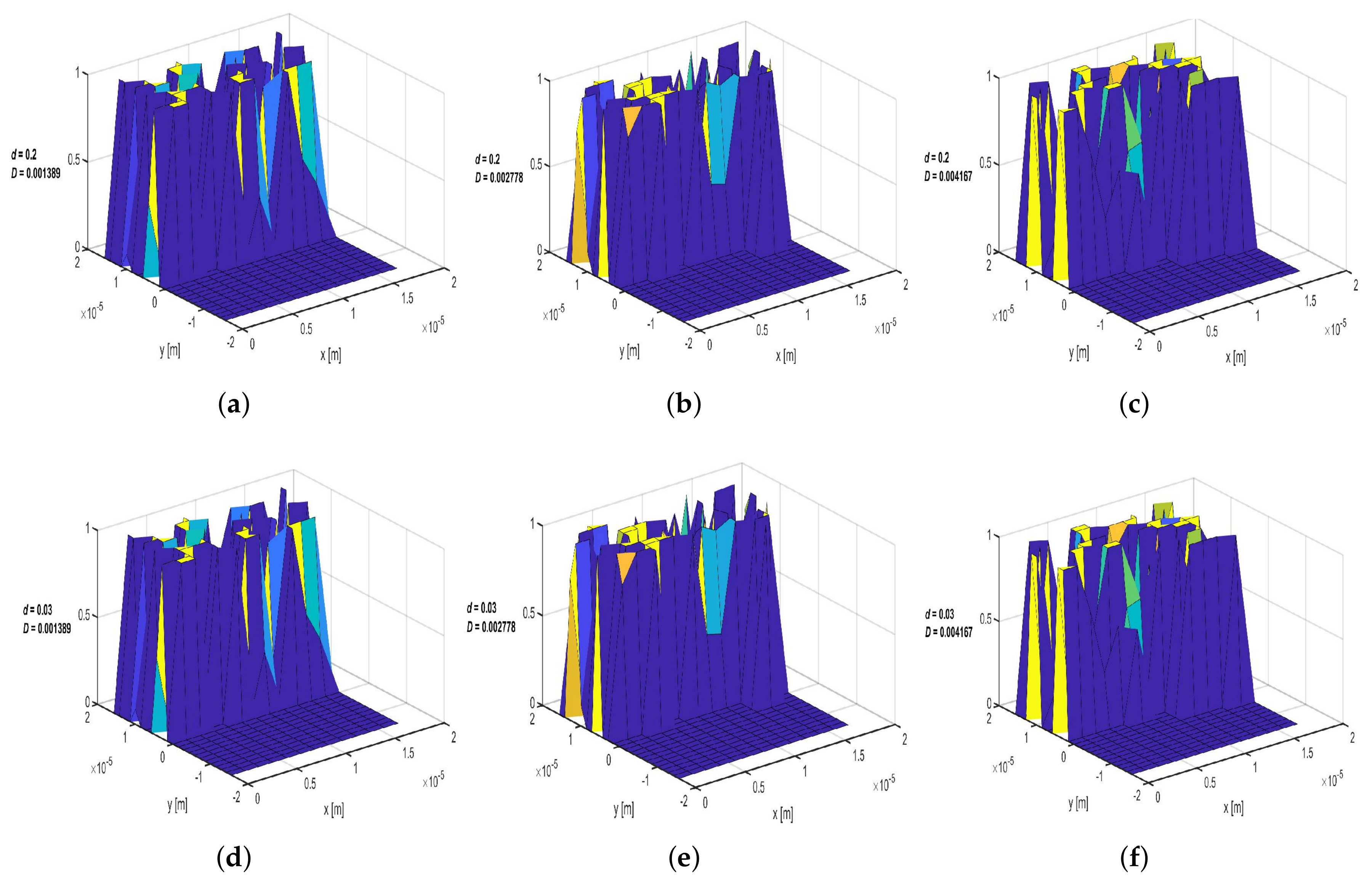
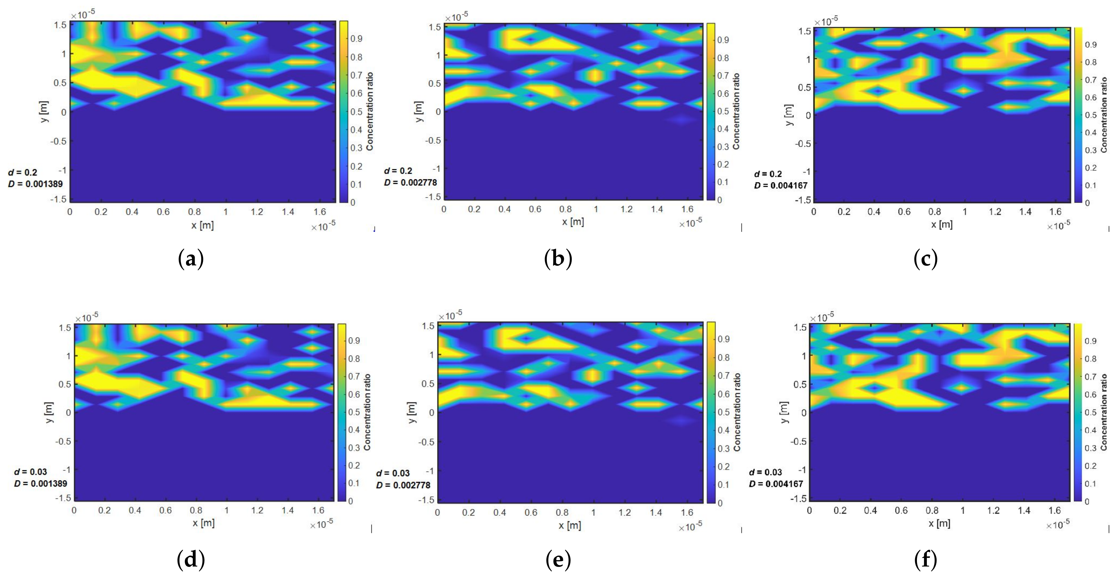
Appendix G. Concentration Distribution within the Porous Media with Linear Drift Ratio d = 0.006, 0.03 and 0.2 at Three Selected Time Intervals (t = 10, 50 and 70 Days) and a Variable Dispersion Coefficient of Do = 0.001389, 0.002778 and 0.004167 m2/s

Appendix G.1. 10 Days

Figure A3. Concentration distribution within the porous media with variable linear drift ratio and dispersion coefficients correspond to (a) d = 0.2, D=0.001389 (b) d = 0.2, D = 0.002778 (c) d = 0.2, D = 0.004167 (d) d = 0.03, D = 0.001389 (e) d = 0.03, D = 0.002778 (f) d = 0.03, D = 0.004167 (g) d = 0.06, D = 0.001389 (h) d = 0.06, D = 0.002778 (i) d = 0.06, D = 0.004167 at a period of 10 days.
Mathematics 09 02509 g0a3aMathematics 09 02509 g0a3b

Appendix G.2. t = 50 Days

Figure A4. Concentration distribution within the porous media with variable linear drift ratio and dispersion coefficients correspond to (a) d = 0.2, D=0.001389 (b) d = 0.2, D = 0.002778 (c) d = 0.2, D = 0.004167 (d) d = 0.03, D = 0.001389 (e) d = 0.03, D=0.002778 (f) d = 0.03, D = 0.004167 (g) d = 0.06, D = 0.001389 (h) d = 0.06, D = 0.002778 (i) d = 0.06, D = 0.004167 at a period of 50 days.
Mathematics 09 02509 g0a4aMathematics 09 02509 g0a4b

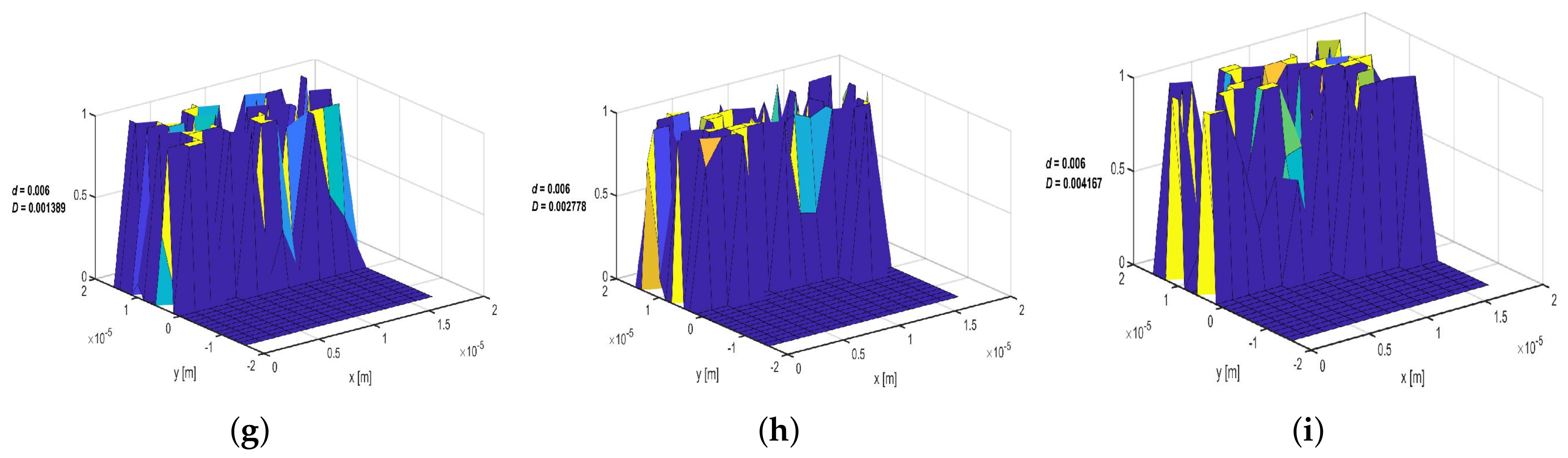
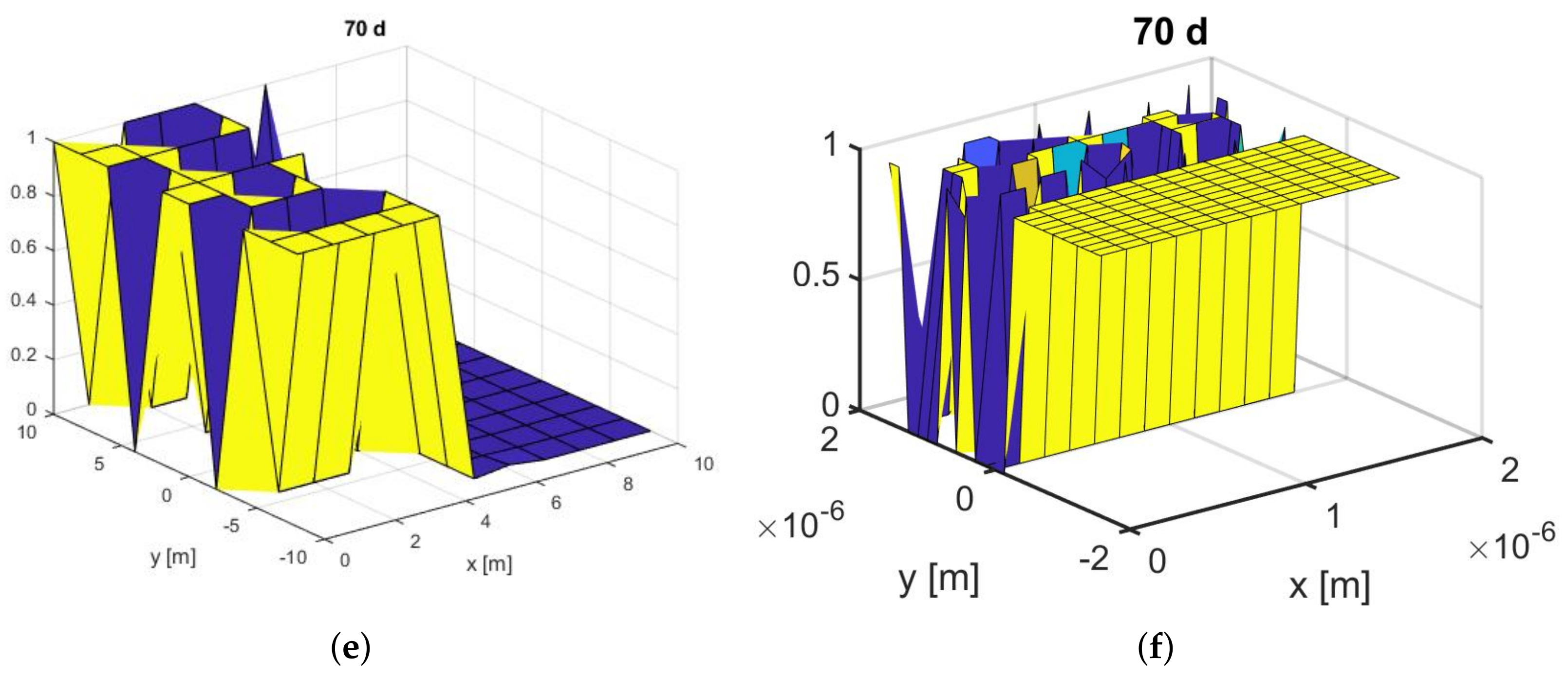
Appendix G.3. t = 70 Days

Figure A5. Concentration distribution within the porous media with variable linear drift ratio and dispersion coefficients correspond to (a) d = 0.2, D = 0.001389 (b) d = 0.2, D = 0.002778 (c) d = 0.2, D = 0.004167 (d) d = 0.03, D = 0.001389 (e) d = 0.03, D = 0.002778 (f) d = 0.03, D = 0.004167 (g) d = 0.06, D = 0.001389 (h) d = 0.06, D = 0.002778 (i) d = 0.06, D = 0.004167 at a period of 70 days.
Mathematics 09 02509 g0a5

References

  1. Ghoraba, S.; Zyedan, B.; Rashwan, I. Solute transport modeling of the groundwater for quaternary aquifer quality management in Middle Delta, Egypt. Alex. Eng. J. 2013, 52, 197–207. [Google Scholar] [CrossRef] [Green Version]
  2. Bekins, B.; Rittmann, B.E.; MacDonald, J.A. Natural attenuation strategy for groundwater cleanup focuses on demonstrating cause and effect, Eos. Trans. Am. Geophys. Union 2001, 82, 53–58. [Google Scholar] [CrossRef] [Green Version]
  3. Offenwert, S.V.; Cnudde, V.; Bultreys, T. Pore-scale visualization and quantification of transient solute transport using fast microcomputed tomography. Water Resour. Res. 2019, 55, 9279–9291. [Google Scholar] [CrossRef] [Green Version]
  4. Axelsson, G. Tracer tests in geothermal resource management. In Proceedings of the EPJ Web of Conferences, Oslo, Norway, 6–8 June 2021; Volume 50 (EDP Sciences), p. 02001. [Google Scholar]
  5. Omofana, E. Effect of Linear Drift on Radial Transport of Tracer in Homogeneous Porous Media. Unpublished Master’s Thesis, African University of Science and Technology, Abuja, Nigeria, 2014; pp. 1–6. [Google Scholar]
  6. Dugstad, O. An Experimental Study of Tracers for Labelling of Injection Gas in Oil Reservoirs. Unpublished Ph.D. Thesis, University of Bergen, Bergen, Norway, 1992; pp. 1–2. [Google Scholar]
  7. Phirani, J.; Roy, S.; Pant, H. Predicting stagnant pore volume in porous media using temporal moments of tracer breakthrough curves. J. Petroleum Sci. Eng. 2018, 165, 640–646. [Google Scholar] [CrossRef]
  8. Dentz, M.; Borgne, T.L.; Englert, A.; Bijeljic, B. Mixing, spreading and reaction in heterogeneous media: A brief review. J. Contam. Hydrol. 2011, 120, 1–17. [Google Scholar] [CrossRef] [PubMed]
  9. Hess, N.J.; Oostrom, M.; Celia, M.A.; Hilpert, M.; Kang, Q.; Pyrak-Nolte, L.J.; Scheibe, T.D.; Tartakovsky, A.M.; Werth, C.J.; Wildenschild, D.; et al. EMSL Pore Scale Modeling Challenge/Workshop; Tech. Rep.; (Pacific Northwest National Lab (PNNL): Richland, WA, USA, 2011. [Google Scholar]
  10. Milligen, B.P.V.; Bons, P.D. Analytical model for tracer dispersion in porous media. Phys. Rev. E 2012, 85, 01130. [Google Scholar] [CrossRef] [PubMed] [Green Version]
  11. Berezhkovskii, A.M.; Skvortsov, A.T. Aris-taylor dispersion with drift and diffusion of particles on the tube wall. J. Chem. Phys. 2013, 139, 084101. [Google Scholar] [CrossRef] [PubMed]
  12. Becker, M. Distinguishing advection, dispersion, and diffusion in fractured bedrock. In Proceedings of the U.S. EPA/NGWA Fractured Rock Conference: State of the Science and Measuring Success in Remediation, Portland, Maine, 13–15 September 2004; pp. 685–693. [Google Scholar]
  13. Mukahal, F.A.; Duffy, B.; Wilson, S. Advection and taylor—Aris dispersion in rivulet flow. Proc. R. Soc. A Math. Phys. Eng. Sci. 2017, 473, 20170524. [Google Scholar] [CrossRef] [Green Version]
  14. Dorfman, K.D.; Brenner, H. Generalized taylor-aris dispersion in discrete spatially periodic networks: Microfluidic applications. Phys. Rev. E 2002, 65, 021103. [Google Scholar] [CrossRef]
  15. Vedel, S.; Bruus, H. Transient taylor-aris dispersion for time-dependent flows in straight channels. J. Fluid Mech. 2012, 691, 95. [Google Scholar] [CrossRef] [Green Version]
  16. Akanji, L.T.; Falade, G.K. Closed-form solution of radial transport of tracers in porous media influenced by linear drift. Energies 2019, 12, 29. [Google Scholar] [CrossRef] [Green Version]
  17. Kuttanikkad, S. Pore-Scale Direct Numerical Simulation of Flow and Transport in Porous Media. Ph.D. Thesis, Ruprecht-Karls-Universitt, Heidelberg, Germany, 2009. [Google Scholar]
  18. Godinez-Brizuela, O.E.; Niasar, V.J. Simultaneous pressure and electro-osmosis driven flow in charged porous media: Pore-scale effects on mixing and dispersion. J. Colloid Interface Sci. 2020, 561, 162–172. [Google Scholar] [CrossRef] [PubMed]
  19. Bear, J. Dynamics of Fluids in Porous Media; Courier Corporation: Washington, DC, USA, 2013. [Google Scholar]
  20. Scheibe, T.D.; Perkins, W.A.; Richmond, M.C.; McKinley, M.I.; Romero-Gomez, P.D.; Oostrom, M.; Wietsma, T.W.; Serkowski, J.A.; Zachara, J.M. Pore-scale and multiscale numerical simulation of flow and transport in a laboratory-scale column. Water Resour. Res. 2015, 51, 1023–1035. [Google Scholar] [CrossRef]
  21. Tsang, Y.; Tsang, C.; Neretnieks, I.; Moreno, L. Flow and tracer transport in fractured media: A variable aperture channel model and its properties. Water Resour. Res. 1988, 24, 2049–2060. [Google Scholar] [CrossRef]
  22. Attinger, S.; Abdulle, A. Effective velocity for transport in heterogeneous compressible flows with mean drift. Phys. Fluids 2008, 20, 016102. [Google Scholar] [CrossRef] [Green Version]
  23. Falade, G.; Brigham, W. Analysis of radial transport of reactive tracer in porous media. SPE Reserv. Eng. 1989, 4, 85–90. [Google Scholar] [CrossRef]
  24. Sanskrityayn, A.; Kumar, N. Analytical solution of advection–diffusion equation in heterogeneous infinite medium using green’s function method. J. Earth Syst. Sci. 2016, 125, 1713–1723. [Google Scholar] [CrossRef]
  25. Aichi, M.; Akitaya, K. Analytical solution for a radial advection–dispersion equation including both mechanical dispersion and molecular diffusion for a steady-state flow field in a horizontal aquifer caused by a constant rate injection from a well. Hydrol. Res. Lett. 2018, 12, 23–27. [Google Scholar] [CrossRef] [Green Version]
  26. Akanji, L.T.; Chidamoio, J. A finite-element algorithm for stokes flow through oil and gas production tubing of uniform diameter. Oil and Gas Science and Technology. Rev. IFP Energies Nouv. 2020, 75, 79. [Google Scholar]
  27. Ayuba, I.; Akanji, T.L.; Gomes, J.L. Velocity Dependence and Tracer Dispersion in Newtonian Fluids Undergoing Creeping Flow. In Proceedings of the SPE Nigeria Annual International Conference and Exhibition, Lagos, Nigeria, 2–4 August 2021. OnePetro. [Google Scholar]
  28. Drazin, P.G.; Riley, N. The Navier-Stokes Equations: A Classification of Flows and Exact Solutions; Cambridge University Press: Cambridge, UK, 2006; p. 334. [Google Scholar]
  29. Abate, J.; Whitt, W. The fourier-series method for inverting transforms of probability distributions. Queueing Syst. 1992, 10, 5–87. [Google Scholar] [CrossRef]
  30. Abate, J.; Whitt, W. Numerical inversion of laplace transforms of probability distributions. ORSA J. Comput. 1995, 7, 36–43. [Google Scholar] [CrossRef] [Green Version]
  31. Gaver, D.P., Jr. Observing stochastic processes, and approximate transform inversion. Oper. Res. 1966, 14, 444–459. [Google Scholar] [CrossRef]
  32. Stehfest, H. Algorithm 368: Numerical inversion of laplace transforms [d5]. Commun. ACM 1970, 13, 47–49. [Google Scholar] [CrossRef]
  33. Talbot, A. The accurate numerical inversion of laplace transforms. IMA J. Appl. Math. 1979, 23, 97–120. [Google Scholar] [CrossRef]
  34. Staben, M.E.; Zinchenko, A.Z.; Davis, R.H. Motion of a particle between two parallel plane walls in low-reynolds-number poiseuille flow. Phys. Fluids 2004, 15, 1711, Erratum in 2004, 16, 4206–4206. [Google Scholar] [CrossRef]
Figure 1. A schematic representation of a chemical tracer in a porous media illustrating (a) the injection of tracer, (b) the reaction between the injected tracer and the injected water bank, (c) the extraction stage without the influence of drift and (df) shows the same process of tracer injection/extraction process displayed in (ac), however, drift effect fully revealed during the extraction stage in (f).
Mathematics 09 02509 g001
Figure 2. A schematic diagram of Poiseuille profile for a 2D channel flow system. In 3D, a surface plane is considered.
Mathematics 09 02509 g002
Figure 3. Normalised channel thickness profile as a function of velocities computed in a spatially heterogeneous porous system.
Mathematics 09 02509 g003
Figure 4. Maximum Reynolds ( R e m a x ) number as a function of maximum velocities ( U m a x ).
Mathematics 09 02509 g004
Figure 5. (af). X-parameter X p as a function of angle θ at a thickness of h = 1.7 × 10 5 m , time t = 10 d and varying separation constant ω 2 . For each channel thickness shown in Figure 3, eleven (11) symmetric velocity data points are generated, and each data point used in the computation of X-parameter X p profiles. Due to the symmetric nature of the velocity profiles, only half-wing of the plane; consisting of six (6) data points, is presented here. The data for the other half-wing is presented in Appendix F.
Mathematics 09 02509 g005
Figure 6. (af). Y- parameter Y p as a function of angle θ at a thickness of h = 1.7 × 10 5 m, time t = 10 d and varying separation constant ω 2 . For each channel thickness shown in Figure 3, eleven (11) symmetric velocity data points are generated, and each data point used in the computation of Y-parameter Y p profiles. Due to the symmetric nature of the velocity profiles, only half-wing of the plane; consisting of six (6) data points, is presented here. The data for the other half-wing is presented in Appendix F.
Mathematics 09 02509 g006
Figure 7. 3D plot of X-parameter X p as a function of the separation constant ω 2 and angle θ at t = 10 d.
Mathematics 09 02509 g007
Figure 8. Contour plots of tracer concentration distribution within the porous media with linear drift ratio d = 0.006, 0.03 and 0.2 at 10 days.
Mathematics 09 02509 g008
Figure 9. Contour plots of tracer concentration distribution within the porous media with linear drift ratio d = 0.006, 0.03 and 0.2 at 50 days.
Mathematics 09 02509 g009
Figure 10. Contour plots of tracer concentration distribution within the porous media with linear drift ratio d = 0.006, 0.03 and 0.2 at 70 days.
Mathematics 09 02509 g010aMathematics 09 02509 g010b
Figure 11. Concentration distribution of tracers at Darcy’s scale within the porous media in (a,c,e) Akanji and Falade 2019 [16] while (b,d,f) shows the result obtained from this pore-scale computation approach of concentration distribution within the porous media with linear drift ratio d = 0.2 and time interval t = 10 d, 50 d, and 70 d.
Mathematics 09 02509 g011aMathematics 09 02509 g011b
Publisher’s Note: MDPI stays neutral with regard to jurisdictional claims in published maps and institutional affiliations.

