Gender Classification Using Proposed CNN-Based Model and Ant Colony Optimization

Abstract

Pedestrian gender classification is one of the key assignments of pedestrian study, and it finds practical applications in content-based image retrieval, population statistics, human–computer interaction, health care, multimedia retrieval systems, demographic collection, and visual surveillance. In this research work, gender classification was carried out using a deep learning approach. A new 64-layer architecture named 4-BSMAB derived from deep AlexNet is proposed. The proposed model was trained on CIFAR-100 dataset utilizing SoftMax classifier. Then, features were obtained from applied datasets with this pre-trained model. The obtained feature set was optimized with ant colony system (ACS) optimization technique. Various classifiers of SVM and KNN were used to perform gender classification utilizing the optimized feature set. Comprehensive experimentation was performed on gender classification datasets, and proposed model produced better results than the existing methods. The suggested model attained highest accuracy, i.e., 85.4%, and 92% AUC on MIT dataset, and best classification results, i.e., 93% accuracy and 96% AUC, on PKU-Reid dataset. The outcomes of extensive experiments carried out on existing standard pedestrian datasets demonstrate that the proposed framework outperformed existing pedestrian gender classification methods, and acceptable results prove the proposed model as a robust model.

1. Introduction

In recent years, researchers’ interest in visual surveillance applications has been growing due to the availability of low-cost optical and infrared cameras and advanced computing machines. Digital cameras are widely used nowadays and deployed on roads, in shopping malls, metro lines and train stations, airports, and residential areas. With digital cameras, pedestrian images are captured under a specific field of view (FoV) in controlled environments [1]. These days, object recognition from images and videos captured by digital cameras is being preferred by people for automated tasks related to security monitoring, public safety [2], pedestrian behavior analysis, etc. Different approaches for video object detection based on deep learning were studied in [3]. Pattern classification from images was also carried out in [4,5,6]. Usually, the movement of different types of objects such as pedestrians takes place in images or video frames. Since pedestrians move in public areas for different purposes such as shopping, to go to work, or to go to school, they are a very important object of real life, and pedestrian-relevant tasks such as pedestrian face recognition [7], pedestrian tracking [8], pedestrian re-identification [9,10,11], action recognition [12,13], and pedestrian gender classification (PGC) [14] are becoming the focus of researchers. Since gender is a key attribute of a pedestrian and plays a role in social communication and human classification (male or female), gender prediction can be useful for various applications related to content-based image retrieval (CBIR), population statistics, human–computer interaction (HCI), health care, multimedia retrieval systems, demographic collection [15], and visual surveillance. Keeping in view the importance of gender prediction in these application areas, pedestrian gender analysis is becoming an imperative field of computer vision. In recent decades, considerable progress has been made in performing the task of gender recognition. Some of the introduced automated gender recognition methods use only low-level information and some others utilize high-level information of images. Low-level information includes hand-crafted features such as shape, color, and texture, while high-level information includes deep features of images [16,17,18,19,20]. These information types also usually use pedestrians’ voices, gait, skin color, and facial expression for gender prediction [21]. However, these approaches have faced issues related to different camera settings, pedestrians’ complex full-body appearances, and variations in their poses. Moreover, environmental effects which include changes in brightness, viewpoint disparities, blur, occlusion, and background cluttering, and images having a low resolution have also affected results while classifying pedestrian gender. Hence, designing a robust method which can effectively automate the process of gender prediction is required. To address the above-mentioned issues of gender prediction, previously proposed methods follow a two-stage classification framework that first extracts features and then carries out classification. Commonly, during the first stage, designing a highly representative feature descriptor is considered for gender, and then a precise binary classifier distinguishing male and female is obtained during the second stage. Naturally, feature representation is required to be discriminative as well as robust. For this, several methods have used facial characteristics using complete faces [22,23,24,25], and various hand-crafted features have been developed utilizing facial images such as histograms of gradients (HOGs) [26], iris codes [27], and local binary patterns (LBPs) [28], for gender recognition. In automated surveillance systems, since poor visible pedestrian face images are captured due to the distance between the camera and pedestrian faces, especially in long-distance conditions, relevant methods produce low gender recognition rates and are not effective for image-based pedestrian gender recognition. Similarly, the approaches which also use face images do not work in scenarios where a camera is used to capture images of pedestrians from their different sides such as back, left, or right side. The reason behind this is that pedestrian images captured in multi-camera environments normally have issues such as scene variations, viewing angle variation, occlusions, blur, and changes in brightness, and due to these issues, it becomes difficult to extract the required face information. Scene variations lead to changes in the background and illumination of an image, while viewpoint variations cause changes in pedestrians’ full-body appearances and postures. Among these issues, viewpoint variation is considered critical because of its impact on diversification in pedestrian full-body appearances and postures, hence making pedestrian gender recognition tasks more difficult. Deep neural network (DNN)-based methods, especially convolutional neural network (CNN)-based classifiers, performed more successfully than hand-crated features in various tasks related to computer vision, as CNN learns and generates effective feature representations from input data under the diverse appearances of gender and various camera settings [29,30]. Some other methods have tackled scene variation issues [31,32,33,34], viewpoint variation concerns [35,36,37,38], both scene and viewpoint variation issues [39], and combinations of aforementioned problems [40,41] for pedestrian gender recognition. However, these methods normally need large-scale datasets for training when learning effective models. Even though both traditional and deep CNN approaches have generated effective benchmark results while performing gender prediction, they are still lacking in terms of challenging issues such as distinct feature representations, an imbalanced distribution of data, lower accuracies, and a small sample space (SSS) for model learning. Regarding these scenarios, the objective of this research work is to develop a new method for pedestrian gender recognition by tackling viewpoint variation concerns for better performance.

In this work, the proposed solution for gender classification provides a robust categorization of full-body view-based pedestrian images. The proposed method is related to offline PGC which utilizes body clues in pedestrian image classification. Four different views such as front, back, side, and mixed are considered for PGC. In this regard, a 64 layer-based CNN model is presented to obtain and learn features. The learned features are then supplied to the optimization approach. The features obtained from this approach are provided to different classifiers for PGC. Keeping in view the fact of non-availability of large datasets of PGC for the training of proposed network, to overcome this issue, a large dataset, i.e., CIFAR-100, was selected to train the proposed model, after which feature sets of testing dataset were extracted from a fully connected layer of proposed CNN-based model. Extensive experimentation was carried out using several variations of optimized feature subsets. From the results obtained, it is observed that an overall accuracy of 85.4% and 92% AUC is achieved on MIT dataset with Fine KNN variant of KNN classifier, and best classification accuracy of 93% is attained on PKU-Reid dataset with Cubic SVM classifier, and selection of a 1000-feature subset. The major contributions are presented below:

•

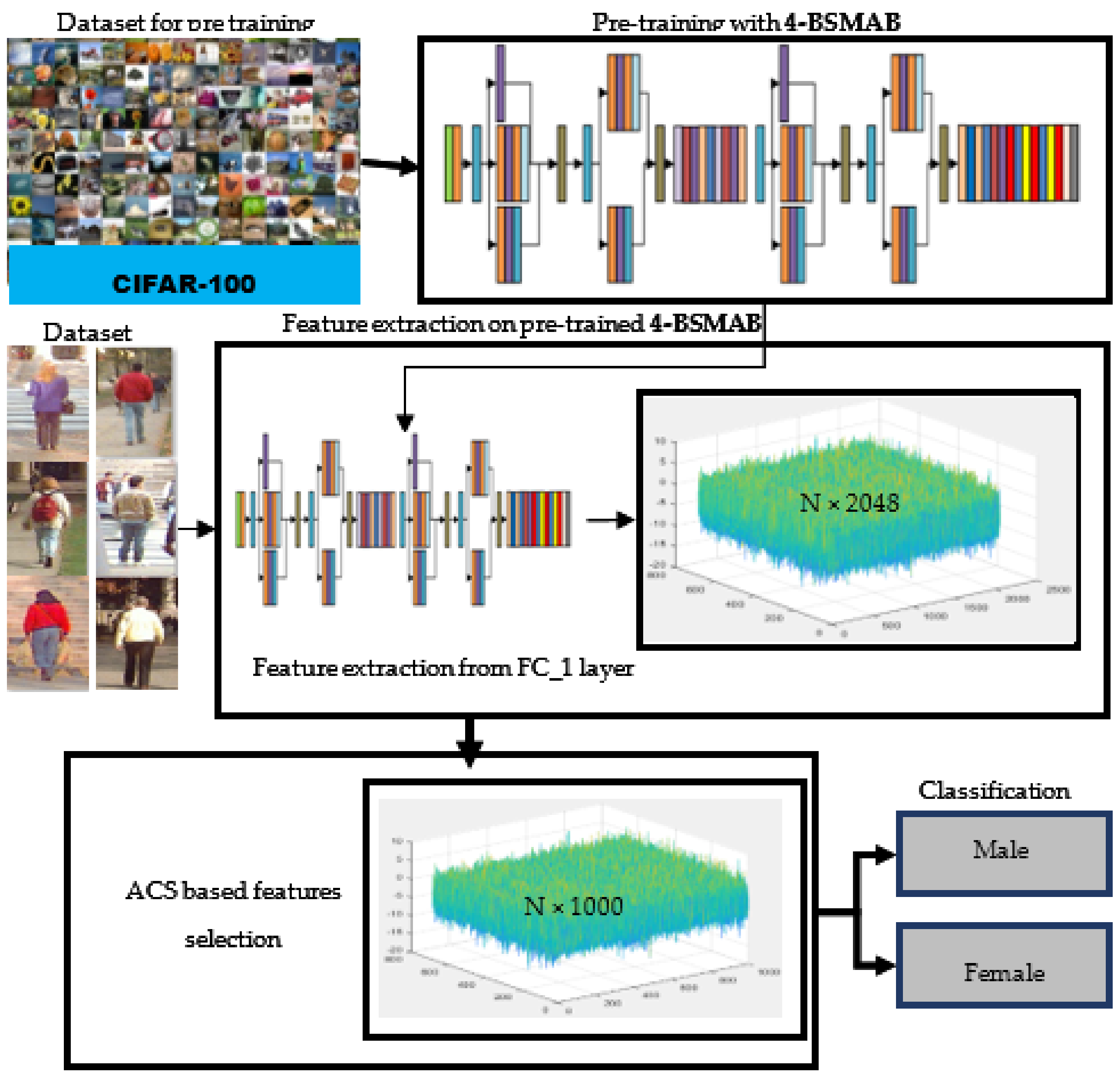
A new architecture based on 64 layers named 4-BSMAB is proposed to obtain features from images. Due to the non-availability of larger datasets, the training of proposed model is carried out on CIFAR-100 dataset, and then the trained model is utilized to extract features from the testing datasets.

•

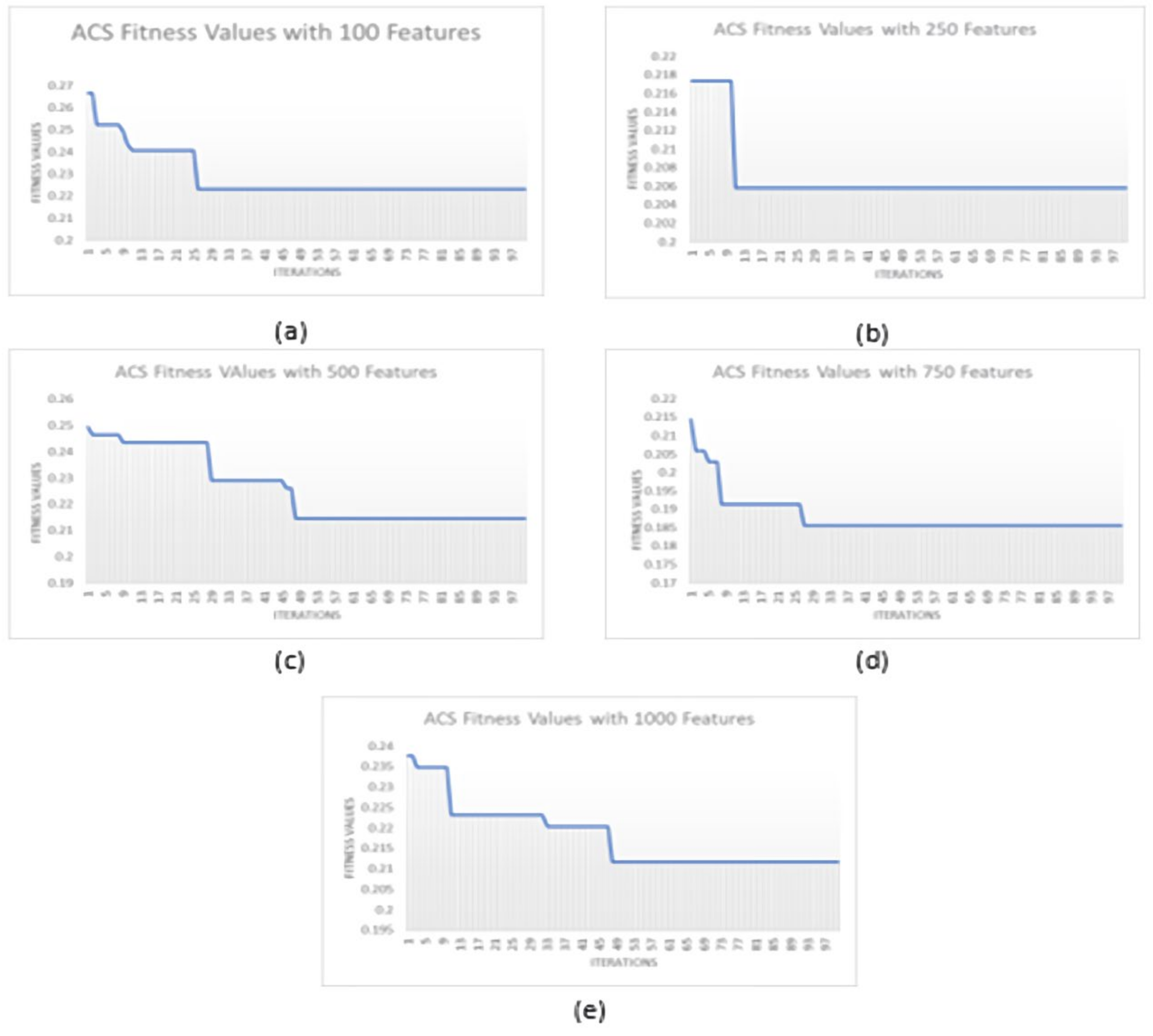
The feature optimization approach (ACS) is applied to obtain features for dimension reduction of extracted features.

•

Various classifiers are tested for PGC, and then the most successful classifier is benchmarked. The classification accuracy achieved with the proposed model shows that the proposed framework is acceptable.

The remaining sections of this manuscript are organized as follows: The Introduction section describes the proposed domain, and next section explains literature review. Section 3 describes the proposed framework. The fourth section provides the results and discusses the details. At the end of this manuscript, this research work is finally concluded.

2. Related Work

In this section, a summary of relevant existing techniques used for gender classification is presented. The following approaches have been proposed for view-based PGC in the relevant literature.

2.1. Traditional/Hand-Crafted Feature-Based Approaches

In this section, a summary of methods that use hand-crafted features for gender classification is highlighted. These approaches use low-level information (features related to shape, color, texture, etc.). For instance, Cao et al. [42] proposed an algorithm named part-based gender recognition (PBGR) utilizing fixed frontal or back views of gender full-body appearance to obtain edge map-based shape information, HOGs, and raw information. They achieved 76.0%, 74.6%, and 75.0% accuracy on front views, back views, and non-fixed views, respectively. Furthermore, Guo et al. [43] utilized front views, back views, and mixed views to investigate biologically inspired features (BIF) from the human body to handle pose variations with support vector machine (SVM). For manifold learning, unsupervised principal component analysis (PCA), supervised orthogonal locality preserving projections (OLPP), marginal Fisher analysis (MFA), and locality-sensitive discriminant analysis (LSDA) were utilized. They achieved 79.5%, 84.0%, and 79.2% accuracy on frontal view with BIF+LSDA, back view with BIF+LSDA, and mixed views with BIF+PCA, respectively, on MIT dataset. Collins et al. [44] extracted features related to spatial pyramid HOGs (PHOGs), local HSV (LHSV) color histograms, spatial pyramid bag of words, etc., and used mixed views from static full-body images to investigate image representations. They obtained 72.2%, 76.0%, and 80.6% overall accuracy on uncropped MIT, cropped MIT, and uncropped VIPeR dataset images, respectively. In addition to above, Geelen et al. [45] first obtained hand-crafted features such as shape, color, and texture from full-body view-based images. Then, a combination of these features was used to perform experiments on MIT CBCL dataset and Datasets A and B for gender classification using SVM and random forest (RF) kernel. They obtained 81.6%, 82.7%, and 80.9% overall accuracy on front views, back views, and mixed views, respectively. They also achieved 79.0%, 79.3%, and 76.6% mean accuracy on front views, back views, and mixed views on MIT dataset. With the above gender classification techniques, although it has been observed that hand-crafted features (low-level feature representations) provide significant resistance against illumination and pose issues, obtaining distinct features from pedestrian full-body views with complex appearances is another challenging issue. Therefore, further investigation of pedestrian full-body views is required to obtain more definite and optimum information for gender classification.

2.2. Deep Learning-Based Approaches

To cope with the problems raised by the traditional hand-crafted feature-based gender classification techniques discussed above such as pedestrians’ diverse appearances and captured images having a low resolution, deep CNN models have been proposed and are considered more appropriate [46,47]. The CNN architecture is popular because of its significant advances in the accuracy obtained in different classification studies [48,49,50]. Currently, trained deep CNN models have been used in a few existing methods for gender prediction. For instance, Ng et al. [16] utilized a CNN model comprising seven layers for issues related to the domain of gender classification. The training of CNN model was carried out on MIT pedestrian dataset for the prediction of gender classification. Overall accuracies of 80.4% and 79.2% were obtained on both front and rear views with a view classifier and without a view classifier, respectively. The proposed approach performed successfully on homogeneous datasets of a small size. Antipov et al. [17] applied mini-CNN and AlexNet-CNN to learn features and compare them with hand-crafted features (HOG) to solve the issue of image feature selection. They found MAP values of 0.80 and 0.85 and AUC values of 0.88 and 0.91 on familiar datasets, while they found MAP values of 0.75 and 0.79 and AUC values of 0.80 and 0.85 on unfamiliar datasets using mini-CNN and AlexNet-CNN. The results showed that the learned features significantly outperformed hand-crafted features for heterogeneous datasets. Ng et al. [18] utilized grayscale, RGB, and YUV color spaces on pedestrians’ full-body images to represent the image for gender prediction with a deep CNN network, which produced significant results on MIT dataset containing pedestrians’ front and rear views. An average accuracy of 81.47% was attained on frontal and rear views with the grayscale color space. Ng et al. [19] further utilized labeled low-level training data and a CNN to introduce a strategy for training. Filters were learned with k-means clustering (unsupervised learning), whereas supervised learning performed pre-training on MIT dataset (front and back views). The training strategy generally performed better than random weight initialization. Raza et al. [20] used appearances from the complete and upper portion of body and deep CNN model for the analysis of pedestrian gender. The existing mechanism for pedestrian parsing was applied to parse both full-body as well as upper-half body-based pedestrian objects in CNN model, after which the SoftMax classifier was applied. The authors achieved 82.1%, 81.3%, and 82.0% overall accuracy and 81.1%, 81.7%, and 80.7% mean accuracy on front views, back views, and mixed views with full-body appearances. They also obtained 83.3%, 82.3%, and 82.8% overall accuracy and 80.5%, 82.3%, and 81.4% mean accuracy on front views, back views, and mixed views with upper-body appearances. Furthermore, Raza et al. [51] also used a deep learning approach and a stacked sparse autoencoder (SSAE) to classify gender. The deep neural network method parsed pedestrian images to remove background, and a two-layer SSAE with SoftMax classifier predicted gender as male or female. The researchers achieved 82.9%, 81.8%, and 82.4% accuracy on front views, back views, and mixed views, respectively, on MIT dataset. They also attained a 91.5% AUC mean value on PETA dataset. Cai et al. [52] investigated and obtained deep features and low-level (HOG) features simultaneously from images by a deep CNN model named as deep-learned and hand-crafted features fusion network (DHFFN) using PCA. After extracting features, fusion is applied to mix both features for exploring their full merits. Experiments on numerous public datasets such as MIT, VIPeR, GRID, PRID, and CHUK were performed, and DHFFN produced 0.95 MAP and 0.95 AUC and was declared a better performer than the state-of-the-art gender prediction methods. Cai et al. [40] further introduced HOG-assisted deep feature learning (HDFL), a novel method that uses a deep CNN to cater common challenges such as viewpoint variations, occlusion, and poor quality faced while predicting gender. HDFL efficiently extracted deep-learned features as well as HOG features simultaneously from the pedestrian picture. A feature fusion process is then applied to extract more discriminative features to provide to SoftMax classifier for gender prediction. The proposed HDFL achieved 0.93 MAP and 0.94 AUC with local response normalization (LRN) and 0.94 MAP and 0.95 AUC with LRN. In earlier gender classification studies, CNN architecture has been used only for considering whole-body images, i.e., global information, but Ng. et al. [53] took global as well as local information from full-body images and introduced a novel parts-based framework that uses a combination of local and global information towards PGC. A local and global CNN method was trained on both whole-body images as well as identified areas of body for feature learning and classification. While comparing the accuracy extracted by utilizing different regions of body such as upper, middle, and lower regions after performing experiments on MIT and APiS datasets, the upper-half body region played a more important role in gender classification as compared to the middle or lower half of body. The authors achieved 84.4%, 88.9%, and 86.8% accuracy utilizing a combination of MIT and APis datasets on frontal, non-frontal, and mixed views, respectively. Fayyaz et al. [41] proposed a hybrid approach that produces a combination of low-level information and deep features of pedestrian images and computes information effectively assisted bya joint feature representation (JFR) scheme for better gender classification tasks. Extensive experiments were performed by adopting different classifiers such as SVM, discriminant classification, and k-nearest neighbor (KNN) to observe sufficient low-level (HOG and LOMO features) and deep feature-based contributions for the design of a JFR, and in this way, the proposed approach achieved 96% AUC and 89.3% accuracy on PETA dataset, and 86% AUC and 82% accuracy on MIT dataset. A study was also conducted by Cai et al. [39] in which the cascading scene and viewpoint feature learning (CSVFL) method improved pedestrian gender recognition. In CSVFL, two crucial challenges, namely, scene and viewpoint variations in pedestrian gender recognition, were jointly considered. The authors demonstrated that CSVFL was able to resist both variations (scene and viewpoint) at the same time. The results generated by CSVFL were also compared with various recent relevant tasks, and an excellent performance was observed. They obtained 84.4%, 85.9%, and 85.2% accuracy utilizing MIT dataset on frontal, back, and mixed views, respectively. They also achieved 81.9%, 84.7%, 72.1%, and 80.1% accuracy utilizing VIPeR dataset on frontal, back, side, and mixed views. Further, 92.4%, 94.6%, 88.2%, and 92.7% accuracy was obtained using PETA dataset on frontal, back, side, and mixed views, respectively.

It can be observed from the results of above-mentioned fine-tuned models that these models are robust, but imbalanced distribution of data is also a challenge while obtaining class-wise accuracy. The above discussion also reflects the fact that full-body view-based pedestrian images are widely investigated for gender classification. All the existing techniques equally applied large-scale and small-scale datasets in experimentation. It has been observed that a fusion approach generates a compact representation of gender images for classification. Moreover, a dataset having a small size is an issue for model learning in deep learning-based approaches.

3. Material and Methods

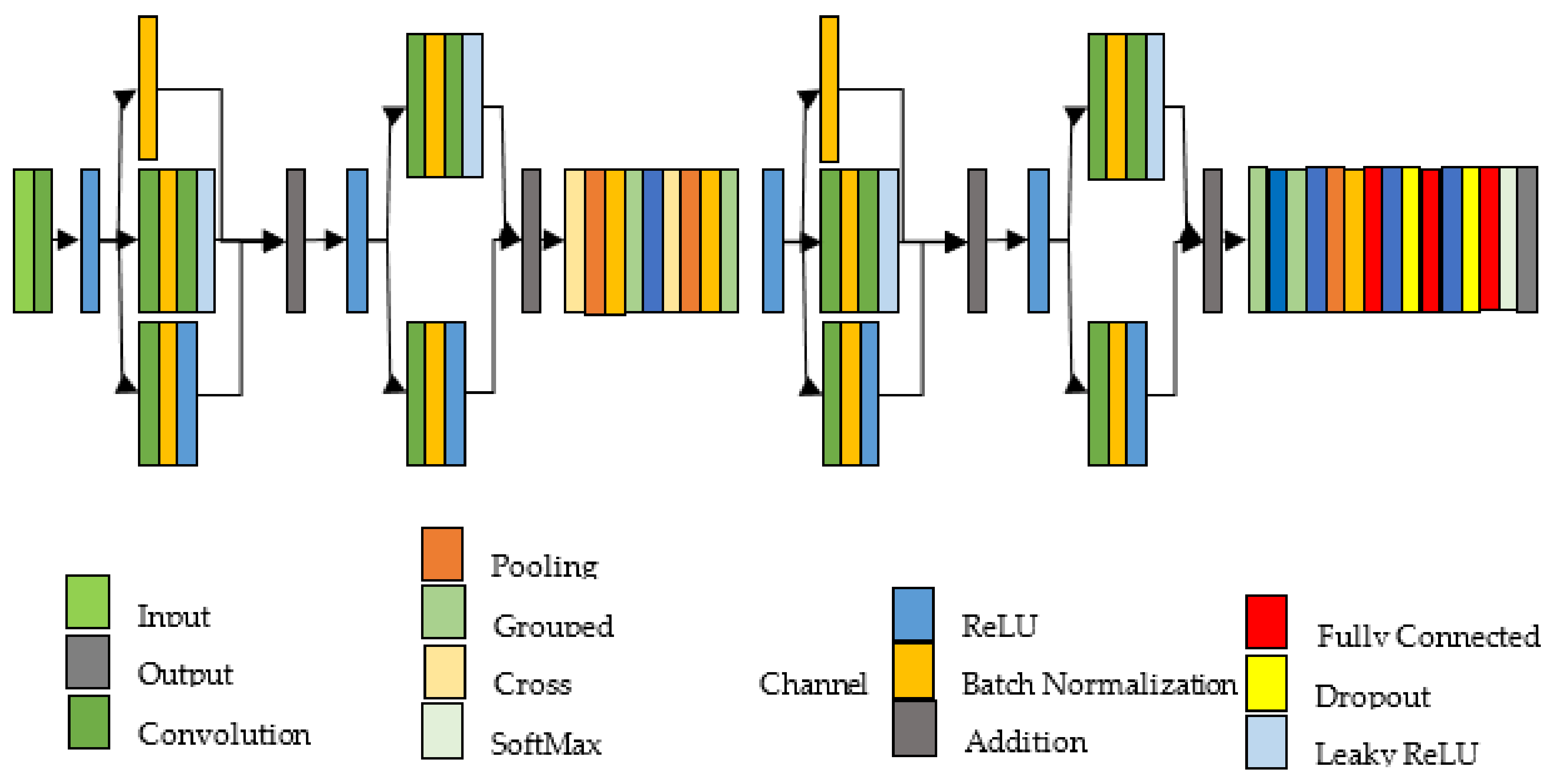
This section presents the proposed model 4-BSMAB and its major steps for PGC. These steps include pre-training of proposed model, dataset balancing, process of feature extraction from 4-BSMAB model, ACS-based feature optimization, and, at the end, classification. An overview of this model is presented in Figure 1. These steps are elaborated in the upcoming section.

3.1. 4-BSMAB

A new architecture, 4-BSMAB (4-branch subnets with modified AlexNet backbone), based on CNN architecture is introduced in this work for PGC. This newly developed model is derived from CNN network named AlexNet [54]. AlexNet contains 25 layers including 5 convolutional layers, 3 fully connected layers, 3 pooling layers, 7 rectified linear unit (ReLU) layers, 2 dropout layers, and SoftMax layers and is divided into 3 repeating blocks named here as R1, R2, and R3. The new model contains 64 layers including input and output layers. The architectural view of proposed model 4-BSMAB is presented in Figure 2, and the details of layers are listed in

Table 1. Configurations of layers of proposed model 4-BSMAB.

Layer #	Layer Name	Feature Maps	Filter Depth	Stride	Padding	Pooling Window Size/Other Values
1	Data	$227\times 227\times 3$
2	C_1	$55\times 55\times 96$	$11\times 11\times 3\times 96$	[4 4]	[0 0 0 0]
3	R1_1	$55\times 55\times 96$
4	C4_1	$55\times 55\times 96$	$5\times 5\times 96\times 96$	[1 1]	Same
5	C2 _1	$55\times 55\times 48$	$1\times 1\times 96\times 48$	[1 1]	Same
6	BN1_1	$55\times 55\times 48$
7	BN2	$55\times 55\times 96$
8	BN3_1	$55\times 55\times 96$
9	LR2_1	$55\times 55\times 96$				Scaling value 0.01
10	C3_1	$55\times 55\times 96$	$11\times 11\times 48\times 96$	[1 1]	Same
11	LR1_1	$55\times 55\times 96$				Scaling value 0.01
12	ADD1_1	$55\times 55\times 96$
13	R1_2	$55\times 55\times 96$
14	C4_2	$55\times 55\times 96$	$5\times 5\times 96\times 96$	[1 1]	Same
15	BN3_2	$55\times 55\times 96$
16	LR2_2	$55\times 55\times 96$				Scaling value 0.01
17	C2_2	$55\times 55\times 48$	$1\times 1\times 96\times 48$	[1 1]	Same
18	BN1_2	$55\times 55\times 48$
19	C3_2	$55\times 55\times 96$	$11\times 11\times 48\times 96$	[1 1]	Same
20	LR1_2	$55\times 55\times 96$				Scaling value 0.01
21	ADD1_2	$55\times 55\times 96$
22	norm1	$55\times 55\times 96$
23	P1	$27\times 27\times 96$		[2 2]	[0 0 0 0]	Maximum pooling $3\times 3$
24	BN4	$27\times 27\times 96$
25	GC1(c5)	$27\times 27\times 256$	Two groups of $5\times 5\times 48\times 128$	[1 1]	[2 2 2 2]
26	R2	$27\times 27\times 256$
27	norm2	$27\times 27\times 256$
28	P2	$13\times 13\times 256$		[2 2]	[0 0 0 0]	Maximum pooling $3\times 3$
29	BN5	$13\times 13\times 256$
30	GC2(c6)	$13\times 13\times 384$	$3\times 3\times 256\times 384$	[1 1]	[1 1 1 1]
31	R3_1	$13\times 13\times 384$
32	BN7	$13\times 13\times 384$
33	C7_1	$13\times 13\times 192$	$1\times 1\times 384\times 192$	[1 1]	Same
34	BN6_1	$13\times 13\times 192$
35	C8_1	$13\times 13\times 384$	$5\times 5\times 192\times 384$	[1 1]	Same
36	LR3_1	$13\times 13\times 384$				Scaling value 0.01
37	C9_1	$13\times 13\times 384$	$3\times 3\times 384\times 384$	[1 1]	Same
38	BN8_1	$13\times 13\times 384$
39	LR4_1	$13\times 13\times 384$				Scaling value 0.01
40	ADD2_1	$13\times 13\times 384$
41	R3_2	$13\times 13\times 384$
42	C7_2	$13\times 13\times 384$	$1\times 1\times 384\times 192$	[1 1]	Same
43	C9_2	$13\times 13\times 384$	$3\times 3\times 384\times 384$	[1 1]	Same
44	BN8_2	$13\times 13\times 384$
45	BN6_2	$13\times 13\times 192$
46	C8_2	$13\times 13\times 384$	$5\times 5\times 192\times 384$	[1 1]	Same
47	LR3_2	$13\times 13\times 384$				Scaling value 0.01
48	LR4_2	$13\times 13\times 384$				Scaling value 0.01
49	ADD2_2	$13\times 13\times 384$
50	GC3(c10)	$13\times 13\times 384$	Two groups of $3\times 3\times 192\times 192$	[1 1]	[1 1 1 1]
51	R4	$13\times 13\times 256$
52	GC4(c11)	$13\times 13\times 256$	Two groups of $3\times 3\times 192\times 128$	[1 1]	[1 1 1 1]
53	R5	$13\times 13\times 256$
54	P3	$6\times 6\times 256$		[2 2]	[0 0 0 0]	Max pooling $3\times 3$
55	BN9	$6\times 6\times 256$
56	Fc_1	$1\times 1\times 2048$
57	R6	$1\times 1\times 2048$
58	D1	$1\times 1\times 2048$				50% Dropout
59	Fc_2	$1\times 1\times 2048$
60	R7	$1\times 1\times 2048$
61	D2	$1\times 1\times 2048$				50% Dropout
62	Fc_3	$1\times 1\times 100$
63	prob	$1\times 1\times 100$
63	Class output

.

The existing network, i.e., AlexNet, was altered with the help of addition of layers, and a new model, 4-BSMAB, is proposed. The batch normalization (BN) layer is included at the end of blocks R1 and R2. Two branched sub-networks are also added along with R blocks. BN1_1 is called first sub-network, and it has three branches. The first branch has a BN tier. The second branch has C2, BN1, C3, and LR1 tiers. The last branch contains layers such as C9, BN8, and LR4. Then, the fusion process is applied on three branches with an addition (ADD) layer. The other sub-network (BN_2) has only two branches. The difference between BN_2 and BN_1 is that BN_1 has only the group BN layer. Two sub-networks such as BN_1 and BN_3 are incorporated at the end of ReLU layer in block R1. Two activation functions are used, i.e., ReLU and Leaky ReLU, at ReLU layer. The ReLU functions are simple and fast and help in speeding up the training phase, and this way, neural networks are also improved. The ReLU functions are easy to compute and do not suffer from vanishing gradients. These functions are implemented with a simple procedure, and due to this characteristic, they are suitable to be used on GPUs.

GPUs are popular and can be improved while carrying out matrix operations. Leaky ReLU functions stop ReLU problems from dying. This type of variation of ReLU produces a small positive slope in the negative area; therefore, it produces possible back-propagation, even for negative input values. Leaky ReLU does not provide steady predictions for input values which are negative. Two sub-networks including BN6_1 and BN8_1 are incorporated at the end of block R2.

The layer details of proposed 4-BSMAB are discussed in the upcoming section. The convolution of input vector $\Vert { }_{j-1 }$ is carried out using a filter bank in C_1 layer. The mathematical form of convolution operation represented by $\ast$ is described as

$${⃦}_{p^{\prime },j}={\mathcal{N}}_j\left({{\displaystyle \sum }}_p{ℌ}_{j,p^{\prime }p}\ast {⃦}_{p,j-1}+{\mathcal{M}}_{p^{\prime },j}\right)$$

(1)

where $p_j$ represents various input channels, and ${p^{\prime }}_j$ represents the number of output channels; the value represented by j indicates the number of layers [55]; $ℌ$ denotes the filter of depth ${p^{\prime }}_j$; and both symbols $\mathcal{M} \mathrm{and} \mathcal{N}$ indicate nonlinear functions. Layers such as group convolution (GC) are also added in 4-BSMAB model. A GC layer is a combination of many convolutional layers. A GC layer enables the procedure of training around GPUs which are in the form of clusters and have a low capacity related to memory. The filters are divided into many splits in a GC layer. A certain range of collection of 2D convolution is carried out by all groups. The mathematical form of layers related to pooling is

$$⃦⃦{ }_{i,j,x,v}={\max }_{l=1\dots s, m=1\dots t} {⃦}_{p,j-1,\left(\mathrm{w}+\mathrm{m}\right)\left(\mathrm{x}+\mathrm{n}\right)}$$

(2)

where $w,x$ represent the index of matrix of image ${\mathbb{I}}_{p,j-1}$, and $m,n$ denote the index of matrix used for the selected pool window. Both norm(s) and BN(s) are utilized in this scheme. BN [56] is a procedure to adjust neurons of the channel over the amount defined for a small batch. Its purpose is to determine both the mean and variance in parts. With the help of a determined mean, the separation of features is carried out with standard deviation. The mean of batch $\mathcal{B}={\mathbb{I}}_1,\dots , {\mathbb{I}}_w$ is calculated as follows:

$$Mea{n}_{\mathcal{B}}=\frac{1}{w}{\displaystyle \sum }_{z=1}^w{\mathbb{I}}_z$$

(3)

where $w$ shows per batch feature maps. The variance is described per batch (small) and is shown as

$$Va{r}_{\mathbb{B}}=\frac{1}{w}{\displaystyle \sum }_{z=1}^w{\left({\mathbb{I}}_z-Mea{n}_{\mathbb{B}}\right)}^2$$

(4)

The below expression is then used forfeature normalization.

$$\widehat{{\mathbb{I}}_Z}=\frac{{\mathbb{I}}_z-Mea{n}_{\mathbb{B}}}{\sqrt{Va{r}_{\mathbb{B}}+\mathcal{D}}}$$

(5)

where $\mathcal{D}$ represents the consistency value, but it remains constant. The norm layer is used for simplification. The norm layer involves scaling pixels with the maximum factor for local prior layers and boosts the spatial-visual quality. The norm equation is

$$\Vert \stackrel{̿}{{\mathbb{I}}_Z}=\frac{{\mathbb{I}}_z}{{\left(ơ+\frac{\beth \ast \Im }{N}\right)}^{\wp }}$$

(6)

where $\stackrel{̿}{{\mathbb{I}}_Z}$ represents the obtained feature map at the end of norm, $\Im$ shows the “sum of square”,$N$ denotes the size of channel, and $ơ, \beth , \mathrm{and} \wp$ represent normalization criteria. The 4-BSMAB model utilizes both R and LR. The standard R transforms numbers less than zero to zero and is shown in [57] as

$${⃦}_{ü ,ȑ}=\max imum(0, ⃦{ }_{ü ,ȑ})$$

(7)

For values below 0, LR has a small slope instead of becoming 0. LR would have ȑ = 0.01ü when ü is negative. Some other works [58,59,60] are also available from which CNN in-depth learning is possible.

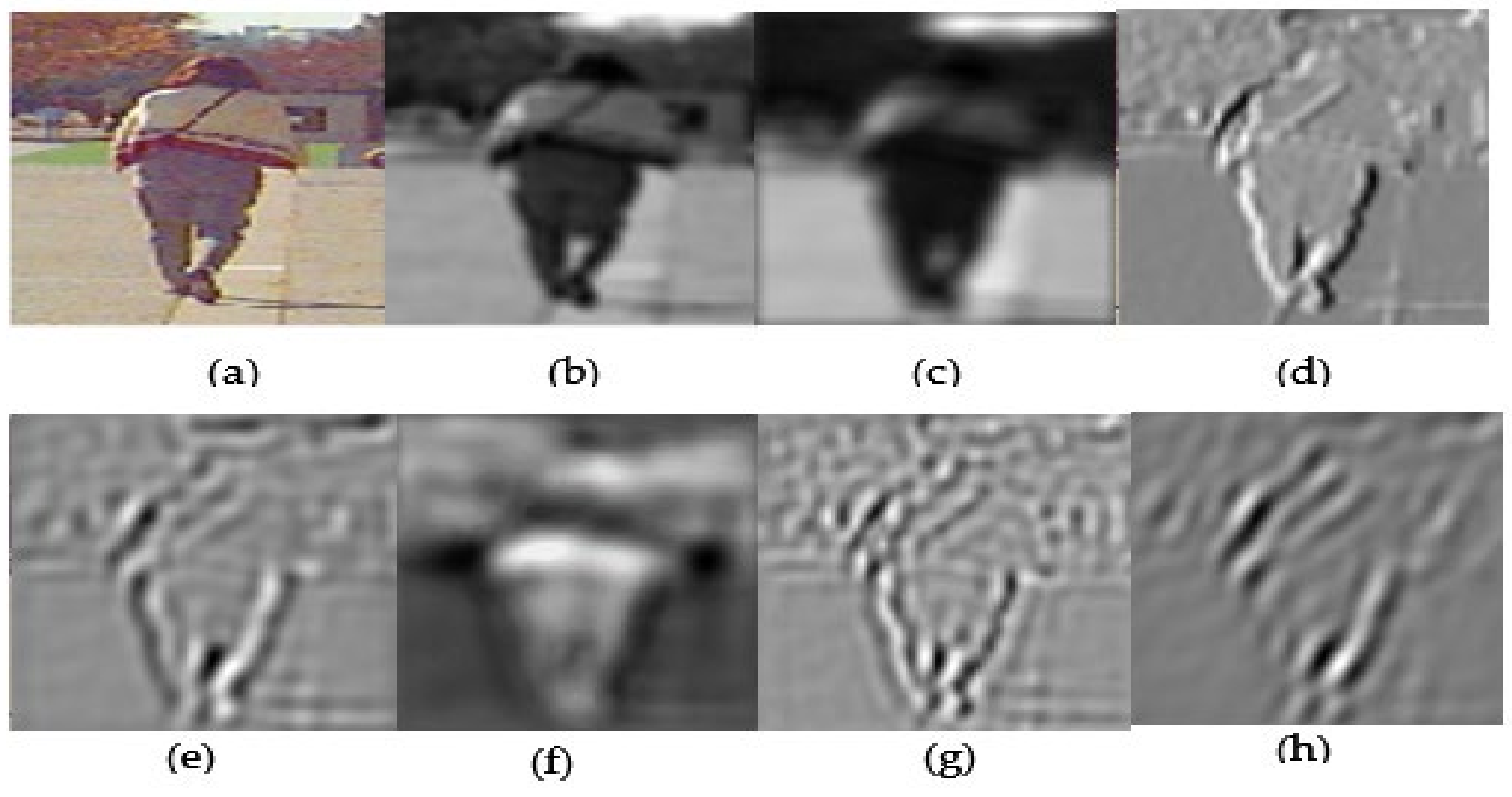
3.2. Pre-Training of Proposed Model and Feature Extraction

The proposed model 4-BSMAB extracts features from the pipeline deeply trained by CNN. The training of proposed model is carried out on a dataset named CIFAR100 [61] having 100 classes of images. In this repository, each class of images is divided into 500 images for model learning and 100 images for model validation. For pre-training, learning images, as well as validation images, are mixed such that each class contains 600 images. The resultant dataset after mixing both types of images of each class is provided to the proposed CNN model for training purposes. The finally trained network is then applied to extract features on pedestrian attribute recognition datasets [41], and FC_1 layer is selected to obtain features. A total of 2048 features are extracted from each image from this layer. This produces a feature set having 418 × 2048, 470 × 2048, and 1728 × 2048 dimensions for frontal views, back views, and mixed views, respectively, for MIT dataset. This also produces a feature set with 590 × 2048, 331 × 2048, and 1264 × 2048 dimensions for frontal views, back views, and mixed views for VIPeR dataset, and feature set dimensions of 684 × 2048, 228 × 2048, and 1640 × 2048 for frontal views, back views, and mixed views for PKU-Reid dataset. Some intermediate visualizations of features captured at various stages of convolution performed by the proposed model 4-BSMAB are shown in Figure 3.

3.3. Feature Selection Based on ACS Optimization

The entropy operation [62] is used to code the obtained features. Entropy $℮$ is usually applied to score the features. Mathematically, entropy has the following form:

$$ё\left( {⃦}^{\prime }{}_1,\dots , {⃦}^{\prime }{}_n\right)=-{{\displaystyle \sum }}_{{\mathfrak{f}}_1}\dots {{\displaystyle \sum }}_{{\mathfrak{f}}_n}P \left({\mathfrak{f}}_1, \dots , {\mathfrak{f}}_n\right) LOG P\left({\mathfrak{f}}_1, \dots , {\mathfrak{f}}_n\right)$$

(8)

where $\left( {\Vert }^{\prime }{}_1,\dots , {\Vert }^{\prime }{}_n\right)$ show the features, $\left({\mathfrak{f}}_1, \dots , {\mathfrak{f}}_n\right)$ represent random variables, and $P\left({\mathfrak{f}}_1, \dots , {\mathfrak{f}}_n\right)$ calculate the probability. ACS is a learning-based approach used for feature optimization. When it is combined with entropy-based feature selection, it becomes an embedded approach. The obtained entropy-coded scores are provided to ACS for feature optimization. The ACS is related to ants’ activities and their movements [63]. Ants move between places and diffuse material called “pheromones”. With time, the material strength decreases gradually. The ants follow the way while calculating the probability of pheromones. This helps ants to select the least expensive path. Therefore, ants’ movement between places is similar to the movement that takes place between vertices of a graph. A graph vertex indicates a feature, and edges from a vertex to another vertex show the selection of features. The strategy repeats to find the best features. The approach stops when minimum number of vertices is traversed and a set criterion is satisfied. The linking arrangement of vertices is similar to a mesh. An ant selects features on a probability basis at a given point at any specified time, and this is written as

$$P_j^m\left(ϯ\right)=\left\{\begin{array}{c}\frac{{\left|h_j\left(\mathfrak{t} \right)\right|}^{ w}{\left|{Ɛ}_j\right|}^w}{{{\displaystyle \sum }}_{v\in ℮\left({{\mathbb{I}}^{\prime }}_1,\dots , {{\mathbb{I}}^{\prime }}_n\right)}{\left|{\mathfrak{h}}_v\left(\mathcal{T}\right)\right|}^{\stackrel{⃛}{\mathfrak{w}}}{\left|{\mathfrak{S}}_v\right|}^{\mathfrak{w}}} if j\in ё\left( {⃦}^{\prime }{}_1,\dots , {⃦}^{\prime }{}_n\right)\\ 0 otherwise\end{array}\right.$$

(9)

where $ё\left({{\mathbb{I}}^{\prime }}_1,\dots , {{\mathbb{I}}^{\prime }}_n\right)$ are entropy-based features, $h_j\left(\mathcal{T}\right)$ is the value of pheromones, ${Ɛ}_j$ shows the empirical value, $\stackrel{⃛}{w}$ is the cost of pheromones, $\mathcal{W}$ represents rational knowledge, and $\mathfrak{t}$ denotes the time limit. $h_j\left(ϯ\right)$ and $Ɛ{ }_j$ are attached to the j^th feature. It is important to mention here that this will be considered an incomplete response if features are not studied up to this point.

3.4. Dataset Balancing

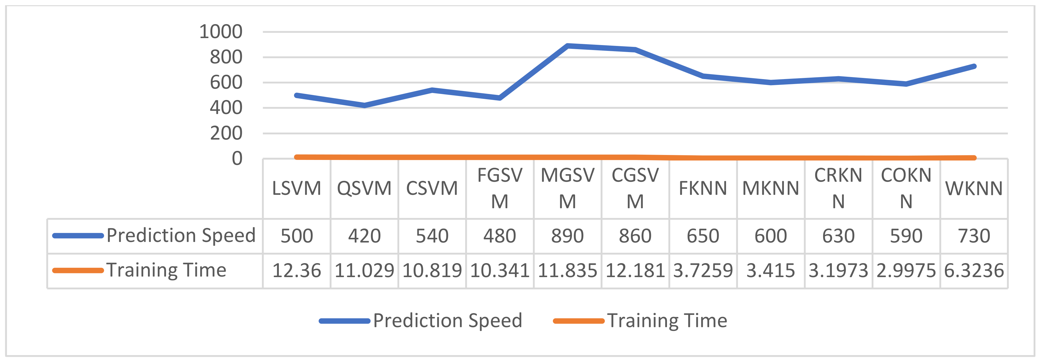
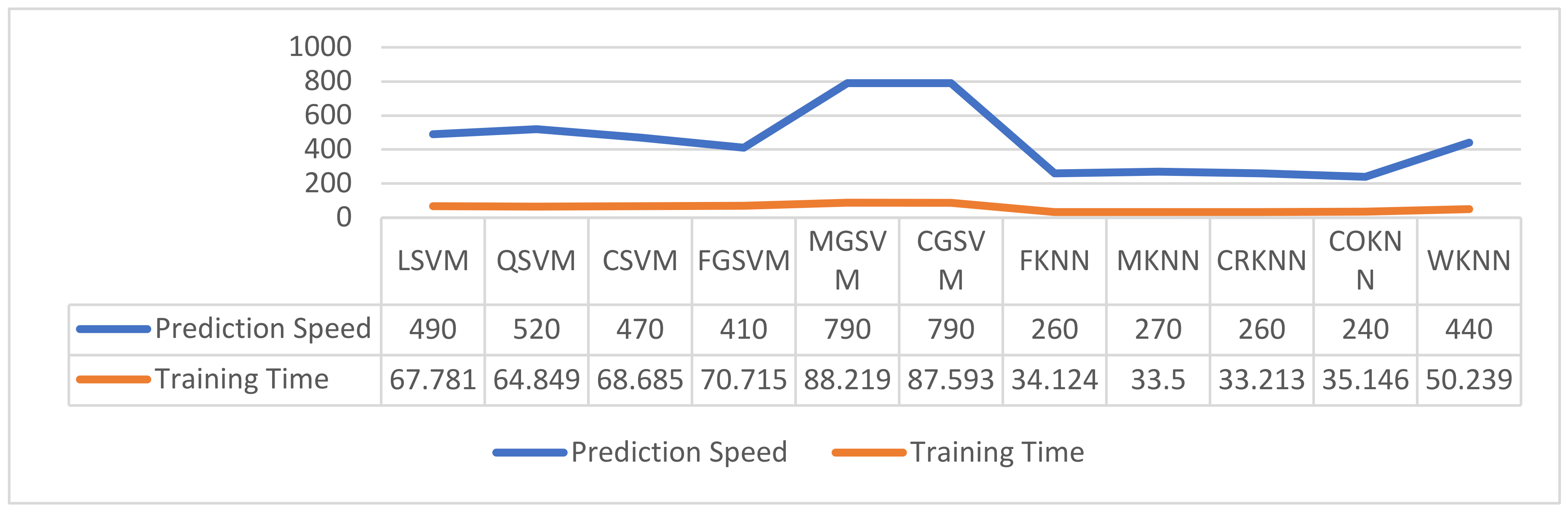
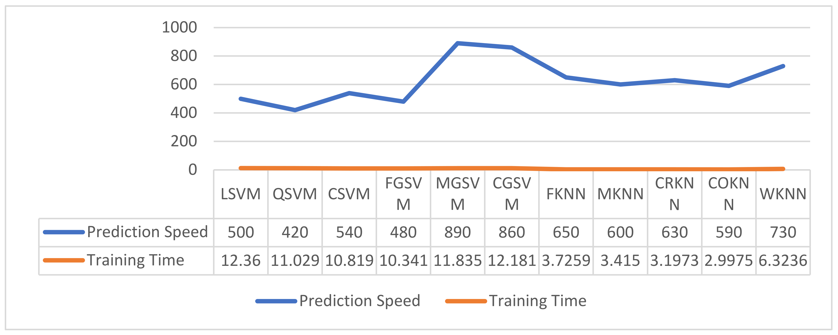
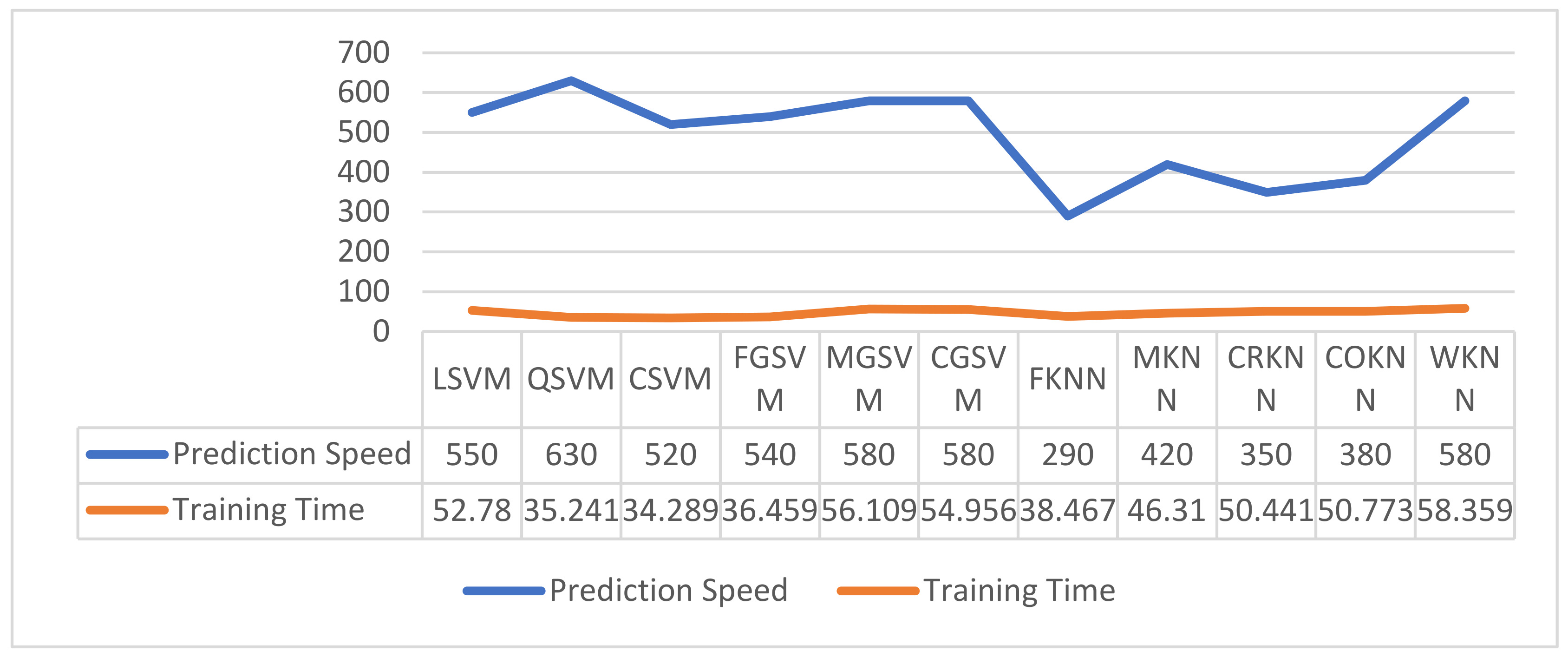
The MIT dataset contains a total of 888 images, out of which 600 are male images and 288 are female images. The number of male and female images is equal in MIT dataset; therefore, this dataset is an imbalanced dataset, leading to the following two research problems: (1) class imbalance problem, which results in poor performance, and (2) small sample space problem, which affects the training of model. Data balancing is selected to enhance the size of dataset and balancing of class-wise data. For this purpose, mirroring and horizontal flipping functions are applied. As a result, 264 male images and 576 female images are added to total 864 male and 864 female images. In this way, the size of MIT dataset is increased and, hence, class-wise data are also balanced.

3.5. Classification

After the selection of features, these are provided to the selected classifiers of SVM [64] and KNN [65] to perform classification. The SVM classifiers include linear variant [66] (LSVM), quadratic variant (QSVM) [67], fine Gaussian variant (FGSVM) [68], medium Gaussian variant (MGSVM), coarse Gaussian (CGSVM), and cubic variant (CSVM) [69]. The details of the kernels of these SVM classifiers can be found in [70,71,72]. The classifiers chosen from KNN include coarse variant (CRKNN), fine variant (FKNN), and cosine variant (COKNN) [73]. The details of these variants are available in [73,74,75,76]. The evaluation of classifiers is conducted on various performance evaluation metrics. Keeping in view the results obtained from experiments, it was observed that CSVM, QSVM, and FKNN classifiers produced better results. FKNN produced highest accuracy with MIT dataset, and CSVM was observed as best classifier in case of PKU-Reid dataset. The details of experiments performed and results produced are presented in the Results section.

4. Results and Discussion

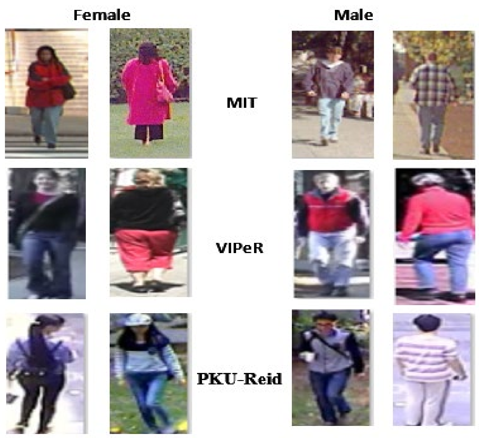
This research was aimed to introduce a novel CNN network based on deep learning to classify pedestrian image datasets. A robust feature set was extracted with the proposed 4-BSMAB CNN-based network, and then various SVM and KNN classifiers were applied to obtain feature sets for evaluating the performance of system. The analysis and outcomes of proposed framework are presented in this section. In the first part, the details of experimental setup along with the datasets used and evaluation protocols applied are provided, and second part explains the experiments performed, which were carried out using a core i5 machine with Windows 10 platform, 8GB memory, and GPU (NVIDIA GTX 1070) with 8GB RAM (inbuilt). The MATLAB2020a tool was selected for programming purposes.

4.1. Datasets

Challenging datasets including viewpoint invariant pedestrian recognition (VIPeR) [77], pedestrian attribute (PETA) [78], cross-dataset [40], MIT [42], and Peking University re-identification (PKU-Reid) [79] were selected to test the proposed approach.

Table 2. Statistics of testing datasets for PGC.

Sr. No.	Datasets	Year	# Images/Videos	Views	Size	Applications
1	VIPeR	2008	1264	Side, Front, Back	128 × 48	Pedestrian re-identification and tracking across multi-camera network
2	MIT	2014	888	Front, Back	128 × 48	Pedestrian attribute analysis
3	PKU-Reid	2016	1824	Side, Front, Back	128 × 48	Pedestrian attribute analysis and re-identification

shows the details of these selected testing datasets. These datasets are also publicly available on the internet for experimental and research work. Different tasks related to pedestrian analysis such as person attribute analysis and PGC have been performed on these datasets. The challenges that exist in these datasets include inter- and intraclass variations (IICV), and environment recording settings (ERS). The IICV consist of speed and style of the movement of pedestrians, and ERS include pose variations, illumination changes, viewpoint changes, recording rates, camera settings, complex backgrounds, object deformation, shadow, and occlusion.

Table 3. View-based sample in MIT, VIPER, PKU-Reid, and PETA datasets used for testing of proposed model.

Type of Views for Testing	MIT		VIPeR		PKU-Reid
	Male	Female	Male	Female	Male	Female
Front	305	113	339	251	420	264
Back	296	174	198	133	140	88
Mixed	864	864	721	543	1120	520

shows view-based information of testing datasets on which the evaluation of proposed model was carried out.

In MIT dataset, 305 male images and 113 female images were selected for front view-based evaluation, 296 male images and 174 female images were selected for backview-based evaluation, and 864 male and 864 female images were selected in case of mixed view-based evaluation. The VIPeR dataset contains 339 male images and 251 female images for front views, 198 male and 133 female images for back views, and 721 male images and 543 female images for mixed views. In PKU-Reid dataset, front views include 420 male and 264 female images, back views include 140 male and 88 female images, and mixed views include 1120 and 520 images of males and females, respectively. Figure 4 shows sample images of males as well as females taken from these datasets.

4.2. Performance Evaluation Protocols

The evaluation of PGC problems directly relates to different accuracies and AUC. In this work, generally used performance evaluation metrics, i.e., accuracy (ACC), receiver operating characteristic (ROC) curve, F-measure (FM), G-measure (GM), area under the curve (AUC), true positive rate (TPR), and false positive rate (FPR), were selected for the measurement of performance of different PGC methods.

Table 4. Performance evaluation metrics.

Sr. No.	Performance Measures	Mathematical Representation
1	FPR	$\frac{FP}{TN+FP}$
2	Sensitivity (SE), TPR, Recall	$\frac{TP}{TP+FN}$
3	Specificity (SP), TNR	$\frac{TN}{TN+FP}$
4	Precision (PR)	$\frac{TP}{TP+FP}$
5	Accuracy (ACC)	$\frac{TP+TN}{TP+TN+FP+FN}$
6	AUC	${{\displaystyle \int }}_{\infty }^{-\infty }TPR\left(t\right)FP{R}^{\prime }\left(t\right)dt$
7	F-Measure (FM)	$2=\frac{Precision X Recall}{Precision X Recall}$
8	G-Measure (GM)	$\sqrt{TPR X TNR}$

shows these metrics with their mathematical representation. Five-fold-type cross-validation was adopted for training and testing.

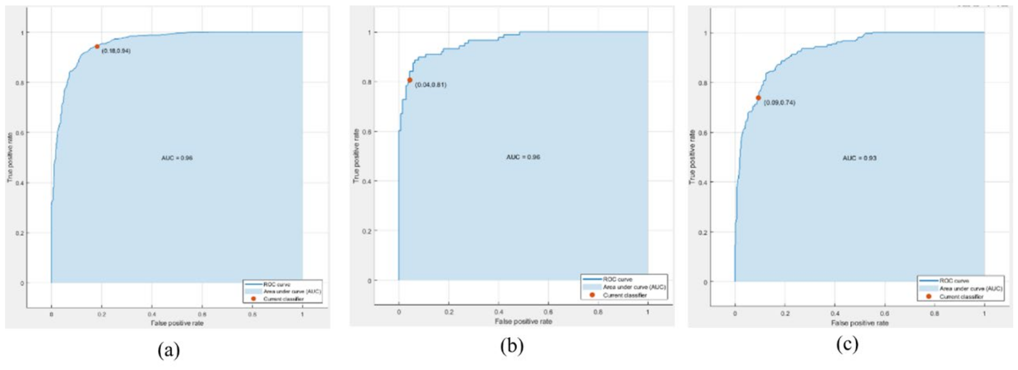
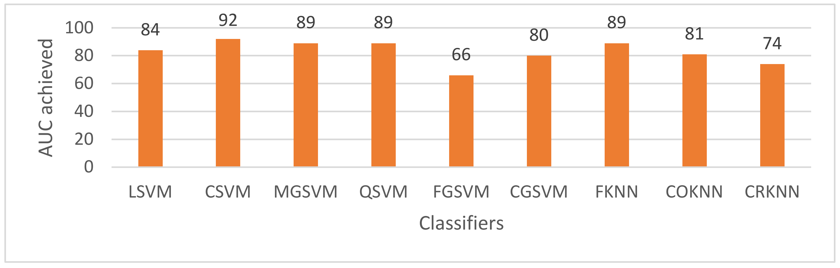
4.3. Performance Evaluation of Proposed Framework

Experiments were performed with the proposed framework on MIT, VIPeR, and PKU-Reid testing datasets to achieve best results. For this purpose, various experiments were carried out with several variations of optimized feature subsets. A major analysis of these experiments is presented in this section.

Table 5. Optimized feature subsets with dimensions and best accuracy on MIT, VIPeR, and PKU-Reid datasets.

Optimized Feature Subset No.	No. of Features	Best ACC (%) Achieved on MIT Dataset			Best ACC (%) Achieved on VIPeR Dataset			Best ACC (%) Achieved on PKU-Reid Dataset
		Front Views	Back Views	Mixed Views	Front Views	Back Views	Mixed Views	Front Views	Back Views	Mixed Views
1	100	74.9	72.8	81.3	65.9	70.0	64.1	79.1	86.8	81.8
2	250	74.6	73.4	84.6	67.0	66.5	68.4	85.7	88.6	88.0
3	500	74.7	73.0	84.7	65.1	69.5	68.3	83.8	89.9	89.8
4	750	74.9	73.8	85.1	69.3	72.5	69.5	84.2	90.4	91.2
5	1000	74.9	73.8	85.4	72.9	70.7	70.3	85.5	93.0	91.2

shows the summary of experiments performed and accuracies produced by them with five feature subsets on front views, back views, and mixed views of selected datasets.

The fitness value graphs obtained by ACS on mixed views of MIT dataset are depicted in Figure 5. The fitness was maintained after 49th iteration, with a value of 0.29, by using 1000-feature subset.

4.3.1. Performance Evaluation of MIT Dataset

In this section, the results generated by experiments performed using front views, back views, and mixed view images of MIT testing dataset are mentioned. Five-fold-type cross-validation was utilized on all feature matrices of MIT dataset obtained from frontal views, back views, and mixed views of MIT dataset and provided to classifiers that are variants of KNN and SVM for automatic labeling. The details of the evaluation of proposed model with five different feature subsets on MIT testing dataset are presented below.

Evaluation of frontal views of MIT dataset: The best result achieved in terms of accuracy was 74.9% by LSVM with 1000-feature subset, CSVM with 750-feature subset, and QSVM with 1000-feature subset, while the second best result attained in terms of accuracy was 74.7% by LSVM with 500-feature subset, as shown in

Table 6. Front view-based experimental results on MIT dataset.

Classification Methods	Optimized Feature Subsets					Evaluation Metrics
	100	250	500	750	1000	ACC	AUC	SE	SP	PR	FM	GM
LSVM					✓	74.9	0.70	99.3	08.9	74.6	85.2	29.7
CSVM				✓		74.9	0.71	91.8	29.2	77.8	84.2	51.8
MGSVM		✓				74.0	0.70	100.0	03.5	74.7	84.8	18.8
QSVM	✓					74.9	0.71	92.5	27.4	77.5	84.3	50.4
QSVM					✓	74.9	0.71	92.5	27.4	77.5	84.3	50.4
FGSVM					✓	73.7	0.52	100.0	02.7	73.5	84.7	16.3
CGSVM					✓	73.2	0.69	100.0	00.9	73.1	84.5	09.4
FKNN				✓		68.9	0.54	82.3	32.7	76.8	79.4	52.0
COKNN			✓			73.2	0.59	96.1	11.5	73.6	84.0	33.2
COKNN					✓	73.2	0.59	95.7	12.4	74.7	84.0	34.4
CRKNN					✓	73.0	0.65	100.0	00.0	73.0	84.4	00.0

. The training time and prediction speed of proposed model on front views of MIT dataset are presented in Figure 6.

Evaluation of back views of MIT dataset: The best accuracy achieved on MIT dataset was 73.8% by CSVM classifier with 1000-feature subset, and QSVM with 750-feature subset, while the second best result obtained in terms of accuracy was 73.4% by QSVM with 250-feature subset, as shown in

Table 7. Back view-based experimental results on MIT dataset.

Classification Methods	Optimized Feature Subsets					Evaluation Metrics
	100	250	500	750	1000	ACC	AUC	SE	SP	PR	FM	GM
LSVM			✓			73.0	0.77	91.2	42.0	72.8	81.0	61.9
CSVM					✓	73.8	0.79	85.1	54.6	76.1	80.4	68.2
MGSVM		✓				70.7	0.78	94.3	305	69.8	80.2	536
QSVM				✓		73.8	0.79	83.8	56.9	76.8	80.1	69.0
FGSVM			✓			63.0	0.53	100.0	00.0	63.0	77.3	00.0
CGSVM					✓	65.8	0.77	99.7	08.1	64.8	78.6	28.3
FKNN				✓		65.1	0.58	74.7	48.9	71.3	73.0	60.4
COKNN		✓				68.3	0.66	84.5	40.8	70.8	77.0	58.7
CRKNN				✓		63.4	0.70	100.0	01.2	63.3	77.5	10.7

. The training time and prediction speed of proposed model on back views of MIT dataset are presented in Figure 7.

Evaluation of mixed views of MIT dataset: The best result achieved in terms of accuracy was 85.3% by FKNN with 1000-feature subset, while the second best result attained in terms of accuracy was 85.1% by FKNN with 750-feature subset, as shown in

Table 8. Mixed view-based experimental results on MIT dataset.

Classification Methods	Optimized Feature Subsets					Evaluation Metrics
	100	250	500	750	1000	Acc	Auc	Se	Sp	PR	FM	GM
LSVM				✓		76.9	0.84	77.0	76.8	77.0	76.9	76.9
CSVM				✓		83.9	0.92	82.6	85.1	84.7	83.7	83.9
MGSVM				✓		81.9	0.89	88.5	75.1	78.1	83.0	81.6
QSVM				✓		81.7	0.89	81.3	82.1	81.9	81.6	81.7
FGSVM	✓					67.3	0.66	95.1	39.4	61.1	74.4	61.2
CGSVM				✓		75.5	0.80	76.7	74.2	74.8	75.8	75.5
FKNN					✓	85.4	0.89	79.9	90.7	89.6	84.5	85.1
COKNN				✓		73.7	0.81	77.3	70.0	72.1	74.6	73.6
CRKNN			✓			67.8	0.74	75.9	59.6	65.3	70.2	67.3

. The training time and prediction speed of proposed model on mixed views of MIT dataset are presented in Figure 8.

The best ROC outcomes on MIT dataset are presented in Figure 9.

4.3.2. Performance Evaluation of VIPeR Dataset

In this section, the results generated by experiments performed using front views, back views, and mixed view images of VIPeR testing dataset are mentioned. Five-fold-type cross-validation was utilized on all feature matrices of MIT dataset obtained from frontal views, back views, and mixed views of VIPeR dataset and provided to classifiers that are variants of KNN and SVM for automatic labeling. The details of the evaluation of proposed model with five different feature subsets on VIPeR testing dataset are presented below.

Evaluation of frontal views of VIPeR dataset: The best result achieved in terms of accuracy was 72.9% by QSVM with 1000-feature subset, while the second best result obtained in terms of accuracy was 70.7% by CSVM with 1000-feature subset, as shown in

Table 9. Front view-based experimental results on VIPeR dataset.

Classification Methods	Optimized Feature Subsets					Evaluation Metrics
	100	250	500	750	1000	ACC	AUC	SE	SP	PR	FM	GM
LSVM				✓		69.3	0.76	82.3	51.8	69.8	75.5	65.3
CSVM					✓	70.7	0.75	78.8	59.8	72.6	75.5	68.6
MGSVM		✓				67.0	0.76	81.7	47.0	67.6	74.0	62.0
QSVM					✓	72.9	0.76	78.8	64.9	75.2	77.0	71.5
FGSVM			✓			57.5	0.57	100.0	00.0	57.5	73.0	00.0
CGSVM					✓	66.8	0.74	91.5	33.5	65.0	76.0	55.3
FKNN				✓		60.3	0.61	69.6	47.8	64.3	66.9	57.7
COKNN					✓	64.8	0.68	80.2	43.8	65.9	72.3	59.3
CRKNN					✓	66.8	0.69	91.5	33.5	65.0	76.0	553

. The training time and prediction speed of proposed model on front views of VIPeR dataset are presented in Figure 10.

Evaluation of back views of VIPeR dataset: The best result achieved in terms of accuracy was 72.5% by QSVM with 750-feature subset, while the second best result attained in terms of accuracy was 70.7% by LSVM with 1000-feature subset, as shown in

Table 10. Back view-based experimental results on VIPeR dataset.

Classification Methods	Optimized Feature Subsets					Evaluation Metrics
	100	250	500	750	1000	ACC	AUC	SE	SP	PR	FM	GM
LSVM					✓	70.7	0.76	86.9	46.6	70.8	78.0	63.7
CSVM	✓					70.0	0.78	80.3	54.1	72.3	76.1	65.9
MGSVM	✓					68.9	0.76	92.9	33.1	67.4	78.1	55.5
QSVM				✓		72.5	0.78	82.8	57.1	74.2	78.3	68.8
FGSVM			✓			59.8	0.51	100.0	00.0	59.8	74.9	00.0
CGSVM					✓	61.9	0.75	99.5	60.2	61.2	75.8	24.5
FKNN			✓			58.3	0.75	68.2	43.6	64.3	66.2	54.5
FKNN					✓	58.3	0.75	64.7	48.9	65.3	65.0	56.2
COKNN					✓	65.0	0.65	79.3	43.6	67.7	73.0	58.8
CRKNN					✓	61.3	0.71	99.5	04.5	60.8	75.5	21.2

. The training time and prediction speed of proposed model on back views of VIPeR dataset are presented in Figure 11.

Evaluation of mixed views of VIPeR dataset: The best accuracy achieved was 70.3% by CSVM with 1000-feature subset, while the second best result obtained in terms of accuracy was 69.5% by LSVM with 750-feature subset, as shown in

Table 11. Mixed view-based experimental results on VIPeR dataset.

Classification Methods	Optimized Feature Subsets					Evaluation Metrics
	100	250	500	750	1000	ACC	AUC	SE	SP	PR	FM	GM
LSVM				✓		69.5	0.74	80.2	55.4	70.5	75.0	66.7
CSVM					✓	70.3	0.74	78.0	60.2	72.2	75.0	68.5
MGSVM			✓			68.3	0.75	84.5	46.8	67.8	75.2	62.9
QSVM					✓	69.1	0.74	78.0	57.3	70.8	74.2	66.9
FGSVM			✓			57.0	0.53	1.00	0.00	57.4	72.7	0.00
CGSVM				✓		68.4	0.73	88.0	42.5	67.0	76.1	61.2
CGSVM					✓	68.4	0.73	83.0	49.2	68.4	75.0	63.9
FKNN	✓					58.4	0.56	66.9	47.2	62.7	64.7	56.1
FKNN		✓				58.4	0.56	66.9	47.2	62.7	64.7	56.0
COKNN				✓		63.2	0.66	72.9	50.5	66.1	69.3	60.7
CRKNN			✓			60.4	0.69	98.5	09.8	59.2	74.0	31.0

. The training time and prediction speed of proposed model on mixed views of VIPeR dataset are presented in Figure 12. The best ROC outcomes on VIPeR dataset are presented in Figure 13.

4.3.3. Performance Evaluation of PKU-Reid Dataset

This section describes the results generated by experiments performed using front views, back views, and mixed view images of PKU-Reid testing dataset. Five-fold-type cross-validation was utilized on all feature matrices of MIT dataset obtained from frontal views, back views, and mixed views of PKU-Reid dataset and provided to classifiers that are variants of KNN and SVM for automatic labeling. The details of the evaluation of proposed model with five different feature subsets on PKU-Reid testing dataset are presented below.

Evaluation of frontal views of PKU-Reid dataset: The best accuracy achieved was 85.7% by CSVM with 250-featuresubset, while the second best accuracy attained was 85.5% by CSVM with 1000-feature subset, as shown in

Table 12. Front view-based experimental results on PKU-Reid dataset.

Classification Methods	Optimized Feature Subsets					Evaluation Metrics
	100	250	500	750	1000	ACC	AUC	SE	SP	PR	FM	GM
LSVM					✓	82.9	0.91	91.2	69.7	82.7	86.8	79.7
CSVM		✓				85.7	0.93	91.2	76.9	86.3	88.7	83.7
MGSVM		✓				82.2	0.92	92.9	65.2	80.9	86.5	77.8
QSVM				✓		84.2	0.92	89.5	75.8	85.5	87.4	82.4
FGSVM			✓			61.4	0.65	100.0	00.0	61.4	76.1	00.0
CGSVM					✓	82.3	0.89	94.8	62.5	80.1	86.8	77.0
FKNN					✓	74.3	0.71	85.2	56.8	75.9	80.3	69.6
COKNN				✓		78.1	0.84	89.3	60.2	78.1	83.3	73.3
CRKNN	✓					66.1	0.84	99.5	12.9	64.5	78.3	35.8
CRKNN				✓		66.1	0.84	98.8	14.0	64.6	78.2	37.2

. The training time and prediction speed of proposed model on front views of PKU-Reid dataset are presented in Figure 14.

Evaluation of back views of PKU-Reid dataset: The best accuracy achieved was 93.0% by CSVM with 1000-feature subset, while the second best result obtained in terms of accuracy was 92.5% by QSVM with 1000-feature subset, as shown in

Table 13. Back view-based experimental results on PKU-Reid dataset.

Classification Methods	Optimized Feature Subsets					Evaluation Metrics
	100	250	500	750	1000	ACC	AUC	SE	SP	PR	FM	GM
LSVM				✓		90.4	0.96	97.1	79.6	88.3	92.5	87.9
CSVM					✓	93.0	0.96	97.9	85.2	91.3	94.5	91.3
MGSVM	✓					86.0	0.95	96.4	69.3	83.3	89.4	81.8
QSVM					✓	92.5	0.96	97.1	85.2	91.3	94.1	91.0
FGSVM			✓			61.4	0.59	100.0	00.0	61.4	76.1	00.0
CGSVM					✓	87.7	0.94	99.3	69.3	83.7	90.9	83.0
FKNN				✓		75.4	0.72	90.7	51.1	74.7	82.0	68.1
COKNN					✓	80.7	0.89	92.1	62.5	79.6	85.4	75.9
CRKNN			✓			61.4	0.85	100.0	00.0	61.4	76.1	00.0

. The training time and prediction speed of proposed model on back views of PKU-Reid dataset are presented in Figure 15.

Evaluation of mixed views of PKU-Reid dataset: The best accuracy achieved was 91.2% by CSVM with 750- and 1000-feature subsets, while the second best result achieved in terms of accuracy was 90.4% by QSVM with 1000-feature subset, as shown in

Table 14. Mixed view-based experimental results on PKU-Reid dataset.

Classification Methods	Optimized Feature Subsets					Evaluation Metrics
	100	250	500	750	1000	ACC	AUC	SE	SP	PR	FM	GM
LSVM					✓	87.4	0.93	88.7	86.0	86.4	87.5	87.3
CSVM				✓		91.2	0.96	91.4	91.0	91.0	91.2	91.2
CSVM					✓	91.2	0.96	91.2	91.2	91.2	91.2	91.2
MGSVM			✓			88.5	0.95	90.5	87.0	87.4	88.7	88.5
QSVM					✓	90.4	0.95	91.1	89.8	89.9	90.5	90.4
FGSVM	✓					56.7	0.59	97.9	15.5	53.7	69.4	39.0
FGSVM		✓				56.7	0.59	97.9	15.5	53.7	69.4	39.0
CGSVM					✓	87.1	0.91	89.1	85.1	85.7	87.3	87.1
FKNN			✓			82.0	0.71	84.0	80.1	80.8	82.4	82.0
COKNN					✓	81.8	0.87	89.7	73.9	77.4	83.1	81.4
CRKNN					✓	79.1	0.87	86.5	71.7	75.4	80.6	78.8

. The training time and prediction speed of proposed model on mixed views of PKU-Reid dataset are presented in Figure 16.

The best ROC outcomes on the PKU-Reid dataset are presentedin Figure 17.

Regarding PKU-Reid dataset, it is pertinent to mention here that the relevant literature has been studied thoroughly to find existing methods in which PKU-Reid dataset is used and results are obtained for PGC purpose, but the literature lacks such methods; hence, a comparison of the results produced by the proposed approach is not possible. Although this dataset was introduced in 2016, researchers have not utilized it for PGC tasks.

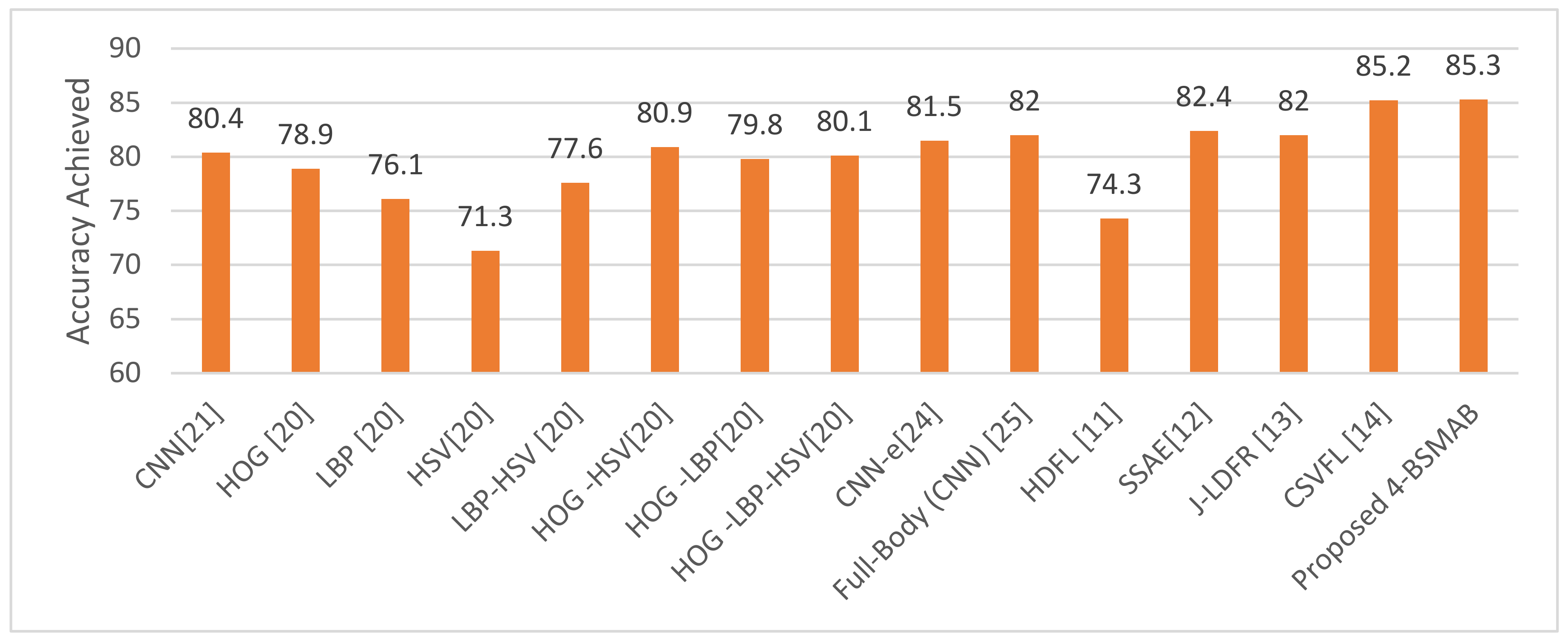
4.4. Performance Comparison between Proposed Approach and Existing Studies

The proposed model was evaluated using frontal views, back views, and mixed views of MIT, VIPeR, and PKU-Reid testing datasets, and details of the results obtained are presented from Table 5, Table 6, Table 7, Table 8, Table 9, Table 10, Table 11, Table 12, Table 13 and Table 14 in the previous section. A performance comparison between the proposed and existing classical and state-of-the-art methods is shown in the upcoming text. The results produced were compared with various methods such as CNN [16], HOG [45], HOG -LBP-HSV [45], CNN-e [19], Full-Body (CNN) [20], HDFL [40], SSAE [51], and recent best performers such as J-LDFR [41] and CSVFL [39] used in PGC for validation of the proposed framework.

These methods were selected for comparison because they have produced results in terms of accuracies on MIT dataset.

Table 15. Performance comparison of results of proposed and existing PGC methods on MIT dataset.

Methods	Year	ACC (%) Using Mixed Views
CNN [16]	2013	80.4
HOG [45]	2015	78.9
LBP [45]	2015	76.1
HSV [45]	2015	71.3
LBP-HSV [45]	2015	77.6
HOG -HSV [45]	2015	80.9
HOG -LBP [45]	2015	79.8
HOG -LBP-HSV [45]	2015	80.1
CNN-e [19]	2017	81.5
Full-Body (CNN) [20]	2017	82.0
HDFL [40]	2018	74.3
SSAE [51]	2018	82.4
J-LDFR [41]	2021	82.0
CSVFL [39]	2021	85.2
Proposed 4-BSMAB	Proposed	85.4

shows the comparison of accuracies achieved by existing pedestrian recognition methods and the proposed approach on MIT dataset. The highest accuracy, i.e., 85.4%, obtained by the proposed framework on MIT dataset was generated by FKNN variant of KNN classifier. It can be observed from Table 15 that the proposed approach shows better accuracy; hence, it outperformed all the existing PGC methods. It accomplished 0.2% better ACC than the latest existing method, CSVFL [39], and 3.3% and 2.9% improvements as compared to the recent best performers J-LDFR [41] and SSAE [51], respectively. By comparing 74.3% accuracy produced by HDFL [40] method with the proposed approach, it can be observed that the proposed method achieved 11.0% higher accuracy. A comparison of the results obtained with the existing and proposed methods in terms of accuracy is shown in Figure 18.

To revalidate the worth of proposed method, the results obtained with the presented approach utilizing AUC evaluation protocol were also compared with existing methods. As per findings from relevant literature, J-LDFR [41] is the only technique that has computed an AUC on mixed views of MIT dataset.

Table 16. AUC performance comparison between proposed and existing PGC approach on MIT dataset.

Methods	Year	AUC (%) Using Mixed Views
J-LDFR [41]	2021	86.0
Proposed 4-BSMAB	Proposed	92.0

shows the comparison in terms of AUC, and obtained results show that the proposed approach outperformed the existing method, J-LDFR [41], with a 6.0% improvement.

Figure 19 shows AUC obtained by the proposed method using various classifiers with 1000-feature subset on mixed views of MIT dataset, and it can be observed that CSVM variant of SVM classifier produced highest AUC of 92.0% on mixed views of MIT dataset.

4.5. Discussion

In this manuscript, PGC problem was addressed, and for this purpose, pedestrian attribute recognition datasets such as MIT, VIPeR, and PKU-Reid were tested. Extensive experiments were performed to develop the proposed approach named as 4-BSMAB, having 64 layers for increased performance. First, CIFAR dataset of 100 classes was used for the training of the proposed model, and then features were extracted from three datasets such as MIT, VIPeR, and PKU-Reid using a pre-trained network. A feature optimization scheme based on ACS was selected to optimize the obtained features. The classification was carried out by performing experiments and selecting various optimal feature subsets, and the outcome of proposed framework was noted with the help of performance evaluation metrics.

At the time of feature selection, different variations of features were defined, and results were obtained applying these variations. The same classifiers were used in all experiments performed. Keeping in view the results obtained with the same classifiers on three different datasets, it was observed that the performance of most utilized classifiers increased as the number of optimized features in feature subsets increased, but, at the same time, the difference in accuracies provided by the classifiers became very small. On the other hand, it was also found that the performance of some classifiers decreased after the first iteration of 100 features and remained the same or increased at a very low rate between second and fourth iterations with feature subsets of 250 to 750, but in the fifth iteration with 1000 features, the performance increased at a very low rate. It was also noted that FKNN, CSVM, QSVM, and sometimes LSVM performed better than the other variants of KNN and SVM, whereas CRKNN, FGSVM, and CGSVM variants showed poor performances in most of the experiments, with a minimum accuracy of nearly 50.0%. The experiments also showed that the performance of most classifiers is better when 500-, 750-, and 1000-feature subsets are used. Overall, 1000-feature subset can be considered best feature subset. It was also seen that the performance of all variants of KNN related to the training time and prediction speed was found to be higher in comparison with SVM.

5. Conclusions

A novel CNN-based framework, 4-BSMAB, was assessed for feature extraction, and ACS was used for the selection of optimized feature sets. The SoftMax classifier was utilized to train 4-BSMAB model on the existing CIFAR-100 dataset, and features were obtained from common pedestrian datasets. An optimized feature set obtained with ACS optimization technique was provided to various classifiers of SVM and KNN for PGC. Five-fold-type cross-validation was carried out to train and test the pedestrian datasets. Extensive experimentation was carried out with various feature subsets, and the details of only five experiments conducted on each dataset were mentioned. It was observed from the experimentation results that the optimized feature subset with 100 features produced a lower accuracy of 81.3%, whereas 1000-featuresubset performed better and achieved 85.4% accuracy with FKNN classifier, and 92% AUC with CSVM classifier, on MIT dataset. A comparison of the results of proposed model and existing state-of-the-art methods on MIT dataset was presented, and it was observed that the proposed method outperformed existing gender classification approaches. It was also noted that CSVM classifier performed better on PKU-Reid dataset and generated 93% accuracy and 96% AUC. The experimentation results also show that most of the classifiers produced better results with 1000-optimized feature subset and obtained second best results with an optimized feature subset of 100 features. As per findings, results on PKU-Reid are not available in the relevant literature, and a performance comparison in this regard is not possible. Although the proposed framework produced satisfactory results, the accuracy can still be improved further. In future work, other approaches such as LSTMs, manifold learning, and quantum deep learning may be explored for better performance.

References

1. Sivabalakrishnan, M.; Menaka, R.; Jeeva, S. Smart video surveillance systems and identification of human behavior analysis. In Countering Cyber Attacks and Preserving the Integrity and Availability of Critical Systems; IGI Global: Philadelphia, PA, USA, 2019; pp. 64–97. [Google Scholar]
2. Filonenko, A.; Jo, K.-H. Unattended object identification for intelligent surveillance systems using sequence of dual background difference. IEEE Trans. Ind. Inform. 2016, 12, 2247–2255. [Google Scholar]
3. Zhu, H.; Wei, H.; Li, B.; Yuan, X.; Kehtarnavaz, N. A Review of Video Object Detection: Datasets, Metrics and Methods. Appl. Sci. 2020, 10, 7834. [Google Scholar] [CrossRef]
4. Jang, D.-H.; Kwon, K.-S.; Kim, J.-K.; Yang, K.-Y.; Kim, J.-B. Dog Identification Method Based on Muzzle Pattern Image. Appl. Sci. 2020, 10, 8994. [Google Scholar] [CrossRef]
5. Rybak, Ł.; Dudczyk, J. A geometrical divide of data particle in gravitational classification of moons and circles data sets. Entropy 2020, 22, 1088. [Google Scholar] [CrossRef]
6. Rybak, Ł.; Dudczyk, J. Variant of Data Particle Geometrical Divide for Imbalanced Data Sets Classification by the Example of Occupancy Detection. Appl. Sci. 2021, 11, 4970. [Google Scholar] [CrossRef]
7. Feng, Q.; Yuan, C.; Pan, J.-S.; Yang, J.-F.; Chou, Y.-T.; Zhou, Y.; Li, W. Superimposed sparse parameter classifiers for face recognition. IEEE Trans. Cybern. 2016, 47, 378–390. [Google Scholar] [CrossRef]
8. Neff, C.; Mendieta, M.; Mohan, S.; Baharani, M.; Rogers, S.; Tabkhi, H. REVAMP 2 T: Real-Time Edge Video Analytics for Multicamera Privacy-Aware Pedestrian Tracking. IEEE Internet Things J. 2019, 7, 2591–2602. [Google Scholar] [CrossRef] [Green Version]
9. Xiao, T.; Li, H.; Ouyang, W.; Wang, X. Learning deep feature representations with domain guided dropout for person re-identification. In Proceedings of the IEEE Conference on Computer Vision and Pattern Recognition, Las Vegas, NV, USA, 27–30 June 2016; pp. 1249–1258. [Google Scholar]
10. Wu, S.; Chen, Y.-C.; Li, X.; Wu, A.-C.; You, J.-J.; Zheng, W.-S. An enhanced deep feature representation for person re-identification. In Proceedings of the 2016 IEEE Winter Conference on Applications of Computer Vision (WACV 2016), Lake Placid, NY, USA, 7–10 March 2016; IEEE: Piscataway, NJ, USA, 2016; pp. 1–8. [Google Scholar]
11. Yao, H.; Zhang, S.; Hong, R.; Zhang, Y.; Xu, C.; Tian, Q. Deep representation learning with part loss for person re-identification. IEEE Trans. Image Process. 2019, 28, 2860–2871. [Google Scholar] [CrossRef] [Green Version]
12. Kong, Y.; Ding, Z.; Li, J.; Fu, Y. Deeply learned view-invariant features for cross-view action recognition. IEEE Trans. Image Process. 2017, 26, 3028–3037. [Google Scholar] [CrossRef]
13. Khan, M.A.; Akram, T.; Sharif, M.; Javed, M.Y.; Muhammad, N.; Yasmin, M. An implementation of optimized framework for action classification using multilayers neural network on selected fused features. Pattern Anal. Appl. 2019, 22, 1377–1397. [Google Scholar] [CrossRef]
14. Ng, C.B.; Tay, Y.H.; Goi, B.-M. Recognizing human gender in computer vision: A survey. In Pacific Rim International Conference on Artificial Intelligence, Kuching, Malaysia, 3–7 September 2012; Springer: Berlin/Heidelberg, Germany, 2012; pp. 335–346. [Google Scholar]
15. Bhatnagar, G.; Wu, Q.J. A fractal dimension based framework for night vision fusion. IEEE/CAA J. Autom. Sin. 2018, 6, 220–227. [Google Scholar] [CrossRef]
16. Ng, C.-B.; Tay, Y.-H.; Goi, B.-M. A convolutional neural network for pedestrian gender recognition. In International Symposium on Neural Networks, Dalian, China, 4–6 July 2013; Springer: Berlin/Heidelberg, Germany, 2013; pp. 558–564. [Google Scholar]
17. Antipov, G.; Berrani, S.-A.; Ruchaud, N.; Dugelay, J.-L. Learned vs. hand-crafted features for pedestrian gender recognition. In Proceedings of the 23rd ACM International Conference on Multimedia, Brisbane, Australia, 26–30 October 2015; ACM: New York, NY, USA, 2015; pp. 1263–1266. [Google Scholar]
18. Ng, C.-B.; Tay, Y.-H.; Goi, B.-M. Comparing image representations for training a convolutional neural network to classify gender. In Proceedings of the 1st International Conference on Artificial Intelligence, Modelling and Simulation, Kota Kinabalu, Malaysia, 3–5 December 2013; IEEE: Piscataway, NJ, USA, 2013; pp. 29–33. [Google Scholar]
19. Ng, C.-B.; Tay, Y.-H.; Goi, B.-M. Training strategy for convolutional neural networks in pedestrian gender classification. In Second International Workshop on Pattern Recognition; International Society for Optics and Photonics: Bellingham, WA, USA, 2017; Volume 10443, p. 104431A. [Google Scholar]
20. Raza, M.; Zonghai, C.; Rehman, S.U.; Zhenhua, G.; Jikai, W.; Peng, B. Part-wise pedestrian gender recognition via deep convolutional neural networks. In Proceedings of the 2nd IET International Conference on Biomedical Image and Signal Processing (ICBISP 2017), Wuhan, China, 13–14 May 2017. [Google Scholar]
21. Sun, Y.; Zhang, M.; Sun, Z.; Tan, T. Demographic analysis from biometric data: Achievements, challenges, and new frontiers. IEEE Trans. Pattern Anal. Mach. Intell. 2017, 40, 332–351. [Google Scholar] [CrossRef]
22. Azzopardi, G.; Greco, A.; Saggese, A.; Vento, M. Fusion of domain-specific and trainable features for gender recognition from face images. IEEE Access 2018, 6, 24171–24183. [Google Scholar] [CrossRef]
23. Mane, S.; Shah, G. Facial recognition, expression recognition, and gender identification. In Data Management, Analytics and Innovation; Springer: Berlin/Heidelberg, Germany, 2019; pp. 275–290. [Google Scholar]
24. Cheng, J.; Li, Y.; Wang, J.; Yu, L.; Wang, S. Exploiting effective facial patches for robust gender recognition. Tsinghua Sci. Technol. 2019, 24, 333–345. [Google Scholar] [CrossRef]
25. Geetha, A.; Sundaram, M.; Vijayakumari, B. Gender classification from face images by mixing the classifier outcome of prime, distinct descriptors. Soft Comput. 2019, 23, 2525–2535. [Google Scholar] [CrossRef]
26. Tapia, J.E.; Perez, C.A. Gender classification based on fusion of different spatial scale features selected by mutual information from histogram of LBP, intensity, and shape. IEEE Trans. Inf. Forensics Secur. 2013, 8, 488–499. [Google Scholar] [CrossRef]
27. Tapia, J.E.; Perez, C.A.; Bowyer, K.W. Gender classification from the same iris code used for recognition. IEEE Trans. Inf. Forensics Secur. 2016, 11, 1760–1770. [Google Scholar] [CrossRef]
28. Shan, C. Learning local binary patterns for gender classification on real-world face images. Pattern Recognit. Lett. 2012, 33, 431–437. [Google Scholar] [CrossRef]
29. Lemley, J.; Bazrafkan, S.; Corcoran, P. Deep Learning for Consumer Devices and Services: Pushing the limits for machine learning, artificial intelligence, and computer vision. IEEE Consum. Electron. Mag. 2017, 6, 48–56. [Google Scholar] [CrossRef] [Green Version]
30. Ahmad, K.; Sohail, A.; Conci, N.; de Natale, F. A comparative study of global and deep features for the analysis of user-generated natural disaster related images. In Proceedings of the IEEE 13th Image, Video, and Multidimensional Signal Processing Workshop (IVMSP), Aristi Village, Greece, 10–12 June 2018; IEEE: Piscataway, NJ, USA, 2018; pp. 1–5. [Google Scholar]
31. Deng, W.; Zheng, L.; Ye, Q.; Kang, G.; Yang, Y.; Jiao, J. Image-image domain adaptation with preserved self-similarity and domain-dissimilarity for person re-identification. In Proceedings of the IEEE Conference on Computer Vision and Pattern Recognition, Salt Lake City, UT, USA, 18–23 June 2018; pp. 994–1003. [Google Scholar]
32. Tang, Y.; Yang, X.; Wang, N.; Song, B.; Gao, X. CGAN-TM: A novel domain-to-domain transferring method for person re-identification. IEEE Trans. Image Process. 2020, 29, 5641–5651. [Google Scholar] [CrossRef]
33. Wei, L.; Zhang, S.; Gao, W.; Tian, Q. Person transfer gan to bridge domain gap for person re-identification. In Proceedings of the IEEE Conference on Computer Vision and Pattern Recognition, Salt Lake City, UT, USA, 18–23 June 2018; pp. 79–88. [Google Scholar]
34. Ren, C.-X.; Liang, B.; Ge, P.; Zhai, Y.; Lei, Z. Domain adaptive person re-identification via camera style generation and label propagation. IEEE Trans. Inf. Forensics Secur. 2019, 15, 1290–1302. [Google Scholar] [CrossRef] [Green Version]
35. Karanam, S.; Li, Y.; Radke, R.J. Person re-identification with discriminatively trained viewpoint invariant dictionaries. In Proceedings of the IEEE International Conference on Computer Vision, Santiago, Chile, 7–13 December 2015; pp. 4516–4524. [Google Scholar]
36. Li, S.; Shao, M.; Fu, Y. Person re-identification by cross-view multi-level dictionary learning. IEEE Trans. Pattern Anal. Mach. Intell. 2017, 40, 2963–2977. [Google Scholar] [CrossRef] [PubMed]
37. Xu, D.; Chen, J.; Liang, C.; Wang, Z.; Hu, R. Cross-view identical part area alignment for person re-identification. In Proceedings of the ICASSP 2019-2019 IEEE International Conference on Acoustics, Speech and Signal Processing (ICASSP), Brighton, UK, 12–17 May 2019; pp. 2462–2466. [Google Scholar]
38. Chen, Y.-C.; Zhu, X.; Zheng, W.-S.; Lai, J.-H. Person re-identification by camera correlation aware feature augmentation. IEEE Trans. Pattern Anal. Mach. Intell. 2017, 40, 392–408. [Google Scholar] [CrossRef] [Green Version]
39. Cai, L.; Zeng, H.; Zhu, J.; Cao, J.; Wang, Y.; Ma, K.-K. Cascading Scene and Viewpoint Feature Learning for Pedestrian Gender Recognition. IEEE Internet Things J. 2020, 8, 3014–3026. [Google Scholar] [CrossRef]
40. Cai, L.; Zhu, J.; Zeng, H.; Chen, J.; Cai, C.; Ma, K.-K. Hog-assisted deep feature learning for pedestrian gender recognition. J. Frankl. Inst. 2018, 355, 1991–2008. [Google Scholar] [CrossRef]
41. Fayyaz, M.; Yasmin, M.; Sharif, M.; Raza, M. J-LDFR: Joint low-level and deep neural network feature representations for pedestrian gender classification. Neural Comput. Appl. 2021, 33, 361–391. [Google Scholar] [CrossRef]
42. Cao, L.; Dikmen, M.; Fu, Y.; Huang, T.S. Gender recognition from body. In Proceedings of the 16th ACM International Conference on Multimedia, Vancouver, BC, Canada, 26–31 October 2008; ACM: New York, NY, USA, 2008; pp. 725–728. [Google Scholar]
43. Guo, G.; Mu, G.; Fu, Y. Gender from body: A biologically-inspired approach with manifold learning. In Proceedings of the Asian Conference on Computer Vision, Xi’an, China, 23–27 September 2009; Springer: Berlin/Heidelberg, Germany, 2009; pp. 236–245. [Google Scholar]
44. Collins, M.; Zhang, J.; Miller, P.; Wang, H. Full body image feature representations for gender profiling. In Proceedings of the 2009 IEEE 12th International Conference on Computer Vision Workshops, ICCV Workshops, Kyoto, Japan, 27 September–4 October 2009; pp. 1235–1242. [Google Scholar]
45. Geelen, C.D.; Wijnhoven, R.G.; Dubbelman, G. Gender classification in low-resolution surveillance video: In-depth comparison of random forests and SVMs. In Video Surveillance and Transportation Imaging Applications; International Society for Optics and Photonics: Bellingham, WA, USA, 2015; Volume 9407, p. 94070M. [Google Scholar]
46. Sindagi, V.A.; Patel, V.M. A survey of recent advances in cnn-based single image crowd counting and density estimation. Pattern Recognit. Lett. 2018, 107, 3–16. [Google Scholar] [CrossRef] [Green Version]
47. Li, C.; Guo, J.; Porikli, F.; Pang, Y. Lightennet: A convolutional neural network for weakly illuminated image enhancement. Pattern Recognit. Lett. 2018, 104, 15–22. [Google Scholar] [CrossRef]
48. Rashid, M.; Khan, M.A.; Sharif, M.; Raza, M.; Sarfraz, M.M.; Afza, F. Object detection and classification: A joint selection and fusion strategy of deep convolutional neural network and SIFT point features. Multimed. Tools Appl. 2019, 78, 15751–15777. [Google Scholar] [CrossRef]
49. Khan, M.A.; Akram, T.; Sharif, M.; Awais, M.; Javed, K.; Ali, H.; Saba, T. CCDF: Automatic system for segmentation and recognition of fruit crops diseases based on correlation coefficient and deep CNN features. Comput. Electron. Agric. 2018, 155, 220–236. [Google Scholar] [CrossRef]
50. Sharif, M.; Khan, M.A.; Rashid, M.; Yasmin, M.; Afza, F.; Tanik, U.J. Deep CNN and geometric features-based gastrointestinal tract diseases detection and classification from wireless capsule endoscopy images. J. Exp. Theor. Artif. Intell. 2019, 33, 1–23. [Google Scholar] [CrossRef]
51. Raza, M.; Sharif, M.; Yasmin, M.; Khan, M.A.; Saba, T.; Fernandes, S.L. Appearance based pedestrians’ gender recognition by employing stacked auto encoders in deep learning. Future Gener. Comput. Syst. 2018, 88, 28–39. [Google Scholar] [CrossRef]
52. Cai, L.; Zhu, J.; Zeng, H.; Chen, J.; Cai, C. Deep-learned and hand-crafted features fusion network for pedestrian gender recognition. In Proceedings of the ELM-2016, Singapore, 13–15 December 2016; Springer: Berlin/Heidelberg, Germany, 2018; pp. 207–215. [Google Scholar]
53. Ng, C.-B.; Tay, Y.-H.; Goi, B.-M. Pedestrian gender classification using combined global and local parts-based convolutional neural networks. Pattern Anal. Appl. 2018, 22, 1469–1480. [Google Scholar] [CrossRef]
54. Krizhevsky, A.; Sutskever, I.; Hinton, G.E. Imagenet classification with deep convolutional neural networks. Adv. Neural Inf. Process. Syst. 2012, 25, 1097–1105. [Google Scholar] [CrossRef]
55. Balocco, S.; González, M.; Ñanculef, R.; Radeva, P.; Thomas, G. Calcified plaque detection in IVUS sequences: Preliminary results using convolutional nets. In Proceedings of the International Workshop on Artificial Intelligence and Pattern Recognition, Havana, Cuba, 24–26 September 2018; Springer: Berlin/Heidelberg, Germany, 2018; pp. 34–42. [Google Scholar]
56. Ioffe, S.; Szegedy, C. Batch normalization: Accelerating deep network training by reducing internal covariate shift. In Proceedings of the International Conference on Machine Learning, Lille, France, 6–11 July 2015; pp. 448–456. [Google Scholar]
57. Liu, Y.; Wang, X.; Wang, L.; Liu, D. A modified leaky ReLU scheme (MLRS) for topology optimization with multiple materials. Appl. Math. Comput. 2019, 352, 188–204. [Google Scholar] [CrossRef]
58. Bouvrie, J. Notes on convolutional neural networks; MIT CBCL Technical Report. Neural Nets 2006, 5869, 47–60. [Google Scholar]
59. Li, Y.; Hao, Z.; Lei, H. Survey of convolutional neural network. J. Comput. Appl. 2016, 36, 2508–2515. [Google Scholar]
60. Wu, J. Introduction to convolutional neural networks. In National Key Lab for Novel Software Technology; Nanjing University: Nanjing, China, 2017; Volume 5, p. 23. [Google Scholar]
61. Krizhevsky, A.; Hinton, G. Learning Multiple Layers of Features From Tiny Images; Technical Report; University of Toronto: Toronto, ON, Canada, 2009. [Google Scholar]
62. Dash, M.; Liu, H. Feature selection for clustering. In Pacific-Asia Conference on Knowledge Discovery and Data Mining; Springer: Berlin/Heidelberg, Germany, 2000; pp. 110–121. [Google Scholar]
63. Rashno, A.; Nazari, B.; Sadri, S.; Saraee, M. Effective pixel classification of mars images based on ant colony optimization feature selection and extreme learning machine. Neurocomputing 2017, 226, 66–79. [Google Scholar] [CrossRef]
64. Noble, W.S. What is a support vector machine? Nat. Biotechnol. 2006, 24, 1565–1567. [Google Scholar] [CrossRef]
65. Peterson, L.E. K-nearest neighbor. Scholarpedia 2009, 4, 1883. [Google Scholar] [CrossRef]
66. Chang, Y.-W.; Lin, C.-J. Feature ranking using linear SVM. In Proceedings of the Workshop on the Causation and Prediction Challenge at WCCI 2008, Hong Kong, China, 3–4 June 2008; pp. 53–64. [Google Scholar]
67. Dagher, I. Quadratic kernel-free non-linear support vector machine. J. Glob. Optim. 2008, 41, 15–30. [Google Scholar] [CrossRef]
68. Virdi, P.; Narayan, Y.; Kumari, P.; Mathew, L. Discrete wavelet packet based elbow movement classification using fine Gaussian SVM. In Proceedings of the IEEE 1st International Conference on Power Electronics, Intelligent Control and Energy Systems (ICPEICES), Delhi, India, 4–6 July 2016; pp. 1–5. [Google Scholar]
69. Liu, Z.; Zuo, M.J.; Zhao, X.; Xu, H. An Analytical Approach to Fast Parameter Selection of Gaussian RBF Kernel for Support Vector Machine. J. Inf. Sci. Eng. 2015, 31, 691–710. [Google Scholar]
70. Rüping, S. SVM Kernels for Time Series Analysis; Technical Report; TU Dortmund: Dortmund, Germany, 2001; pp. 1–13. [Google Scholar] [CrossRef]
71. Ayat, N.-E.; Cheriet, M.; Suen, C.Y. Automatic model selection for the optimization of SVM kernels. Pattern Recognit. 2005, 38, 1733–1745. [Google Scholar] [CrossRef]
72. Haasdonk, B. Feature space interpretation of SVMs with indefinite kernels. IEEE Trans. Pattern Anal. Mach. Intell. 2005, 27, 482–492. [Google Scholar] [CrossRef] [Green Version]
73. Xu, Y.; Zhu, Q.; Fan, Z.; Qiu, M.; Chen, Y.; Liu, H. Coarse to fine K nearest neighbor classifier. Pattern Recognit. Lett. 2013, 34, 980–986. [Google Scholar] [CrossRef]
74. Singh, A.P. Analysis of variants of KNN algorithm based on preprocessing techniques. In Proceedings of the 2018 International Conference on Advances in Computing, Communication Control and Networking (ICACCCN), Greater Noida, India, 12–13 October 2018; pp. 186–191. [Google Scholar]
75. Lamba, A.; Kumar, D. Survey on KNN and its variants. Int. J. Adv. Res. Comput. Commun. Eng. 2016, 5, 430–435. [Google Scholar]
76. Jiang, L.; Zhang, H.; Su, J. Learning k-nearest neighbor naive bayes for ranking. In Proceedings of the International Conference on Advanced Data Mining and Applications, Guilin, China, 19–21 December 2005; Springer: Berlin/Heidelberg, Germany, 2005; pp. 175–185. [Google Scholar]
77. Gray, D.; Tao, H. Viewpoint invariant pedestrian recognition with an ensemble of localized features. In Proceedings of the Computer Vision–ECCV 2008, Marseille, France, 12–18 August 2008; ACM: New York, NY, USA, 2008; pp. 262–275. [Google Scholar]
78. Deng, Y.; Luo, P.; Loy, C.C.; Tang, X. Pedestrian attribute recognition at far distance. In Proceedings of the 22nd ACM International Conference on Multimedia, Orlando, FL, USA, 3–7 November 2014; ACM: New York, NY, USA, 2014; pp. 789–792. [Google Scholar]
79. Ma, L.; Liu, H.; Hu, L.; Wang, C.; Sun, Q. Orientation driven bag of appearances for person re-identification. arXiv 2016, arXiv:1605.02464. [Google Scholar]
Figure 1. Proposed 4-BSMAB model for pedestrian gender classification.
Mathematics 09 02499 g001
Figure 2. Architectural view of proposed model 4-BSMAB.
Mathematics 09 02499 g002
Figure 3. 4-BSMAB best activation visualizations of an image at various convolutional layers: (a) original image; (b) C1_1; (c) C2_1; (d) C2_2; (e) C3_1; (f) C3_2; (g) C4_2; (h) C7_1.
Mathematics 09 02499 g003
Figure 4. Some images of males and females from MIT, VIPeR, and PKU-Reid datasets.
Mathematics 09 02499 g004
Figure 5. Fitness values of ACS-based optimization with (a) 100-feature, (b) 250-feature, (c) 500-feature, (d) 750-feature, and (e) 1000-feature subsets.
Mathematics 09 02499 g005
Figure 6. Proposed model training time (s) and prediction speed (obs/s) on front views of MIT dataset utilizing 1000-feature subset.
Mathematics 09 02499 g006
Figure 7. Proposed model training time (s) and prediction speed (obs/s) on back views of MIT dataset utilizing 1000-feature subset.
Mathematics 09 02499 g007
Figure 8. Proposed model training time (s) and prediction speed (obs/s) on mixed views of MIT dataset utilizing 1000-feature subset.
Mathematics 09 02499 g008
Figure 9. ROC curves and AUC values showing best outcomes of (a) mixed views with CSVM, (b) back views with QSVM, and (c) front views with QSVM of MIT dataset utilizing 1000-feature subset.
Mathematics 09 02499 g009
Figure 10. Proposed model training time (s) and prediction speed (obs/s) on front views of VIPeR dataset utilizing 1000-feature subset.
Mathematics 09 02499 g010
Figure 11. Proposed model training time (s) and prediction speed (obs/s) on back views of VIPeR dataset utilizing 1000-feature subset.
Mathematics 09 02499 g011
Figure 12. Proposed model training time (s) and prediction speed (obs/s) on mixed views of VIPeR dataset utilizing 1000-feature subset.
Mathematics 09 02499 g012
Figure 13. ROC curves and AUC values showing best outcomes of (a) mixed views with MGVM, (b) back views with CSVM, and (c) front views with QSVM of IPeR dataset utilizing 1000-feature subset.
Mathematics 09 02499 g013
Figure 14. Proposed model training time (s) and prediction speed (obs/s) on front views of PKU-Reid dataset utilizing 1000-feature subset.
Mathematics 09 02499 g014
Figure 15. Proposed model training time (s) and prediction speed (obs/s) on back views of PKU-Reid dataset utilizing 1000-feature subset.
Mathematics 09 02499 g015
Figure 16. Proposed model training time (s) and prediction speed (obs/s) on mixed views of PKU-Reid dataset utilizing 1000-feature subset.
Mathematics 09 02499 g016
Figure 17. ROC curves and AUC values showing best outcomes of (a) mixed views with CSVM, (b) back views with CSVM, and (c) front views with CSVM of PKU-Reid dataset utilizing 1000-feature subset.
Mathematics 09 02499 g017
Figure 18. Comparison of accuracy obtained with proposed and existing approaches on MIT dataset.
Mathematics 09 02499 g018
Figure 19. Comparison in terms of AUC with various classifiers on mixed views of MIT dataset using 1000-feature subset.
Mathematics 09 02499 g019