Dynamic Susceptibility of Ferrofluids: The Numerical Algorithm for the Inverse Problem of Magnetic Granulometry

Abstract

The size-dependent properties of magnetic nanoparticles (MNP) are the major characteristics, determining MNP application in modern technologies and bio-medical techniques. Direct measurements of the nanosized particles, involved in intensive Brownian motion, are very complicated; so the correct mathematical methods for the experimental data processing enable to successfully predict the properties of MNP suspensions. In the present paper, we describe the fast numerical algorithm allowing to get the distribution over the relaxation time of MNP magnetic moments in ferrofluids. The algorithm is based on numerical fitting of the experimentally measured frequency spectra of the initial dynamic magnetic susceptibility. The efficiency of the algorithm in the solution of the inverse problem of magnetic granulometry is substantiated by the computer experiments for mono- and bi-fractional ferrofluids.

1. Introduction

Magnetic fluids (or ferrofluids) are stable colloidal suspensions of magnetic nanoparticles (MNP) in a nonmagnetic carrier liquid. The ability to tune the various physical properties of magnetic fluids with applied magnetic fields has led to manifold applications [1] in modern technologies. One important property is the dynamic response of the ferrofluid magnetization to an AC magnetic field. If the field is weak, then the linear response is defined by the initial dynamic magnetic susceptibility, $\chi$, which consists of real (in-phase, ${\chi }^{\prime }$) and imaginary (out-of-phase, ${\chi }^{″}$) parts. Power dissipation is proportional to ${\chi }^{″}$, and so magnetic suspension can be efficiently used in the magnetic hyperthermia method of cancer therapy [2,3,4,5] and the magnetic particle imaging [6,7,8,9].

Magnetic fluids represent a classic paramagnetic system [1]; in the absence of an external magnetic field the total magnetic moment of all MNPs is zero due to their intensive Brownian motion. Applied static magnetic field acts on each MNP magnetic moment turning to rotate it along the field direction, so the fluid static magnetization is always directed along the field. At weak fields,s the magnetization is linear in a field strength, and the initial slope of the magnetization curve defined the initial static magnetic susceptibility of a magnetic fluid. This parameter is of major importance since it determines the magnetic response of a fluid to an applied magnetic field. Evidently, the susceptibility is proportional to the concentration of MNPs and is inverse to temperature and it also defined by a square value of MNP magnetic moment [1]. Since all MNPs are of different sizes, actually the susceptibility is determined by a mean square magnetic moment, which is averaged over the MNP size distribution. In a very strong external field the fluid magnetization approaches the saturation value when all MNP magnetic moments are co-aligned to the field. The saturation magnetization is also proportional to MNP concentration, and it appears to be linear in the mean value of MNP magnetic moment.

Traditionally the researchers try to characterize the nanoparticles with their sizes [10,11,12]. However, here one needs to assume some shape for a nanoparticle and to make some approximations concerning the nanoparticle internal structure. For example, the MNPs are traditionally modeled by the uniformly magnetized spheres, ignoring the MNP non-sphericity and the surface roughness. Ideally, the distribution od MNPs over their sizes can be measured directly with the help of modern experimental techniques, such as Atomic Force Microscopy, or Transmission Electron Microscopy, or Dynamic Light Scattering, etc. However, the problem here is that the MNP is characterized by several sizes. The diameter of metallic nanoparticle is larger than the diameter of magnetized core due to the presence of non-magnetic surface layer of atoms with frustrated spins [1]. In addition, the magnetic suspension is colloidal sterically or electrostatically stabilized. It means the each MNP is covered by a sterical layer of surfactant molecules or by the adsorbed ions forming the double electric layer. These layers increased the hydrodynamic MNP diameter as compared with the size of metallic size nanoparticle. So, the direct measurements do not solve the problem of the MNP size distribution. On the other hand, the prediction of the properties of MNP ensemble often does not demand the correct information about the MNP sizes, but it requires the knowledge of some physical characteristics. Talking about the static magnetic properties of ferrofluids we may state that the correct description and prediction can be obtained knowing the distribution of MNP over their magnetic moments only.

For many applications the dynamic magnetic response of the MNPs is more important than the static magnetic properties. In this case, the spectrum of relaxation times of MNP magnetic moments is of principal interest [13]. However, the problem is that the MNP magnetic moment relaxation time cannot be measured directly but only with the help of indirect experimental methods. Moreover, the spectrum of relaxation times of the ensemble of the MNPs with different sizes differs from that for single MNPs due to collective effects [14]. Anyway, the dynamic magnetic granulometry comprises the numerical solution of the inverse problem, when the numeric dataset of experimental points is described with some analytical expression under the condition of minimization of the standard deviation. The main problem here is concerned with the fact that the ferrofluid susceptibility spectrum is produced by all MNPs, distributed continuously over their sizes, magnetic moments and relaxations times. Since the typical value of MNPs in real ferrofluids has the order ∼10${}^{16}$ per cubic centimeter, we may consider this MNP size distribution as the ’continuous’ one from the mathematical point of view. On the other hand, the numerical fitting can be implemented only with a limited number of MNP fractions. Evidently, the correct numerical fitting demands for a rather large number of these fractions. It means that the number of ’degrees of freedom’ in a numerical solution of the inverse problem is very large; and the computation time should be very long. In addition, the large number of ’degrees of freedom’ does not ensure the high accuracy of the extracted characteristics, since the used experimental data cannot be considered as the ’exact’ data; the measurement data are only known to within the experimental errors. In this paper we are focusing on the numerical method of extraction of the relaxation time spectrum from the experimental measurements of the initial dynamic magnetic susceptibility of ferrofluids. The basic theoretical model and the numerical algorithm are described in Section 2. The results of the algorithm application are presented in Section 3 for extraction of the relaxation time spectrum of the model mono-fraction and bi-fraction ferrofluids, the relaxation times of which are known in advance. In addition, we end with our Discussion.

2. Theory

2.1. Theoretical Model

The dynamic magnetic response of a system of non-interacting MNPs at temperature T to a weak linear polarized probing magnetic field is given by the Debye expressions [15] for the initial dynamic magnetic susceptibility, ${\chi }_{\mathrm{D}}\left(f\right)={\chi }_{\mathrm{D}}^{\prime }\left(f\right)-i{\chi }_{\mathrm{D}}^{″}\left(f\right)$:

$${\chi }_{\mathrm{D}}^{\prime }\left(f\right)={\chi }_{\mathrm{L}}\sum _{k=1}^N\frac{A_k}{1+{\left(2\pi f{\tau }_k\right)}^2},$$

(1)

$${\chi }_{\mathrm{D}}^{″}\left(f\right)={\chi }_{\mathrm{L}}\sum _{k=1}^N\frac{A_{k}2\pi f{\tau }_k}{1+{\left(2\pi f{\tau }_k\right)}^2}.$$

(2)

Here, f stands for the frequency on an external AC field; ${\chi }_{\mathrm{D}}^{\prime }$ and ${\chi }_{\mathrm{D}}^{″}$ are the real and the imaginary parts of the Debye dynamic susceptibility, respectively. We consider also that all MNPs are divided into N fractions; each MNP of the k-th fraction is characterized by the same magnetic moment ${\mu }_k$ and the same relaxation time ${\tau }_k$ of this magnetic moment. The total numerical concentration of MNPs is $\rho$, and the molar portion of the k-th fraction is ${\nu }_k$. So, the zero-frequency limit ($f\to 0$) gives the static Langevin susceptibility ${\chi }_{\mathrm{L}}$:

$${\chi }_{\mathrm{L}}=\frac{{\mu }_0\rho }{3k_{\mathrm{B}}T}\sum _{k=1}^N{\mu }_k^2{\nu }_k,\sum _{k=1}^N{\nu }_k=1,$$

(3)

where ${\mu }_0$ is the vacuum permeability; $k_{\mathrm{B}}$ is the Boltzmann’s constant. With these notations the expressions (1) and (2) look like the expansions over the contributions of all N fractions, and the fraction coefficient $A_k$ has the meaning of the amplitude of this contribution:

$$A_k={\mu }_k^2{\nu }_k/\sum _{k=1}^N{\mu }_k^2{\nu }_k,\sum _{k=1}^N{A}_k=1.$$

(4)

It is worth noting here that the MNP distribution over their magnetic moments is unknown in a real experiment, as well as the relaxation time spectrum. So, our goal is to develop the fast and stable numerical algorithm of determination of $A_k$ and ${\tau }_k$ from the AC susceptibility measurements of ferrofluids.

In what follows, for clarity we will describe the algorithm on the basis of Debye model (1) and (2). Applying to real ferrofluids, the Debye expressions may be used for very diluted samples only; this can be measured in terms of Langevin susceptibility, ${\chi }_{\mathrm{L}}\ll 1$. For larger values of ${\chi }_{\mathrm{L}}$, at least comparable with unity, the advanced model should be applied accounting for the interparticle magnetic interaction. For example, the so-called “modified Weiss” (MW) theory [16] might be recommended, the dynamic susceptibility ${\chi }_{\mathrm{MW}}\left(f\right)$ in the framework of which is expressed through the Debye susceptibility

$${\chi }_{\mathrm{MW}}\left(f\right)=\frac{\left(1+\frac{1}{3}{\chi }_{\mathrm{L}}\right){\chi }_{\mathrm{D}}\left(f\right)}{1+\frac{1}{3}{\chi }_{\mathrm{L}}-\frac{1}{3}{\chi }_{\mathrm{D}}\left(f\right)}.$$

(5)

The real, ${\chi }_{\mathrm{MW}}^{\prime }$, and imaginary, ${\chi }_{\mathrm{MW}}^{″}$, parts of this function are

$$\frac{{\chi }_{\mathrm{MW}}^{\prime }\left(f\right)}{\left(1+\frac{1}{3}{\chi }_{\mathrm{L}}\right)}=\frac{\left(1+\frac{1}{3}{\chi }_{\mathrm{L}}\right){\chi }_{\mathrm{D}}^{\prime }\left(f\right)-\frac{1}{3}\left\{{\left[{\chi }_{\mathrm{D}}^{\prime }\left(f\right)\right]}^2+{\left[{\chi }_{\mathrm{D}}^{″}\left(f\right)\right]}^2\right\}}{{\left[1+\frac{1}{3}{\chi }_{\mathrm{L}}-\frac{1}{3}{\chi }_{\mathrm{D}}^{\prime }\left(f\right)\right]}^2+\frac{1}{9}{\left[{\chi }_{\mathrm{D}}^{″}\left(f\right)\right]}^2},$$

(6)

$$\frac{{\chi }_{\mathrm{WM}}^{″}\left(f\right)}{\left(1+\frac{1}{3}{\chi }_{\mathrm{L}}\right)}=\frac{\left(1+\frac{1}{3}{\chi }_{\mathrm{L}}\right){\chi }_{\mathrm{D}}^{″}\left(f\right)}{{\left[1+\frac{1}{3}{\chi }_{\mathrm{L}}-\frac{1}{3}{\chi }_{\mathrm{D}}^{\prime }\left(f\right)\right]}^2+\frac{1}{9}{\left[{\chi }_{\mathrm{D}}^{″}\left(f\right)\right]}^2}.$$

(7)

The MW theory describes very accurately the Brownian dynamic simulation data [16] for the dynamic susceptibility of polydisperse dipolar fluids up to the values of ${\chi }_{\mathrm{L}}\sim 3$. The main physical effect, predicted by the MW theory, is that the system of interacting MNPs exhibits the spectrum of collective relaxation times, differing from the single MNP spectrum ${\tau }_k$ due to the collective effect of interparticle magnetic interaction. As a result, the maximum of the imaginary susceptibility shifts towards lower frequencies with the growth of MNP concentration. This effect was discovered theoretically [14], and then proved by the computer simulations [16,17] and the experimental observations [18,19]. Note that the MW dynamic susceptibility (5) is expressed in terms of the Debye susceptibilities (1) and (2), and thus it is the function of the fraction relaxation times ${\tau }_k$ and the fraction amplitudes $A_k$. This point is very important because the use of the extended MW model (instead of the simple Debye one) does not introduce any additional unknown parameters that need to be determined.

2.2. Numerical Algorithm

The main idea is to extract the information about the relaxation time spectrum of MNP ensemble from the experimental data on the dynamic initial magnetic susceptibility of ferrofluid on the basis of numerical processing of these data with the help of theoretical MW expressions (6) and (7). However, the determination of the coefficients in the relations (6) and (7) from the experimental data is an inverse problem. It relates to an ill-posed problem in the mathematical sense, because the task may not have a unique solution owning to nonlinearity. Moreover, the result of the fitting is dependent on the number of MNP fractions N; and the number of unknown variables is $2N$ (the relaxation times ${\tau }_k$ and the amplitudes $A_k$). However, the computing time grows rapidly with the number of fractions; and the non-linear character of expressions (6) and (7) often makes impossible the numerical solution of the fitting problem with a large number of fractions because it requires a lot of computational resources (computation time). The additional difficulty is connected with the fact of existing measurement errors: the set of experimental points cannot be considered as the exact data. So, some measurement error in one experimental point may lead to an uncontrolled shift in fitting parameters.

To achieve the appropriate computation time and to minimize the influence of experimental errors we suggest the following numerical algorithm.

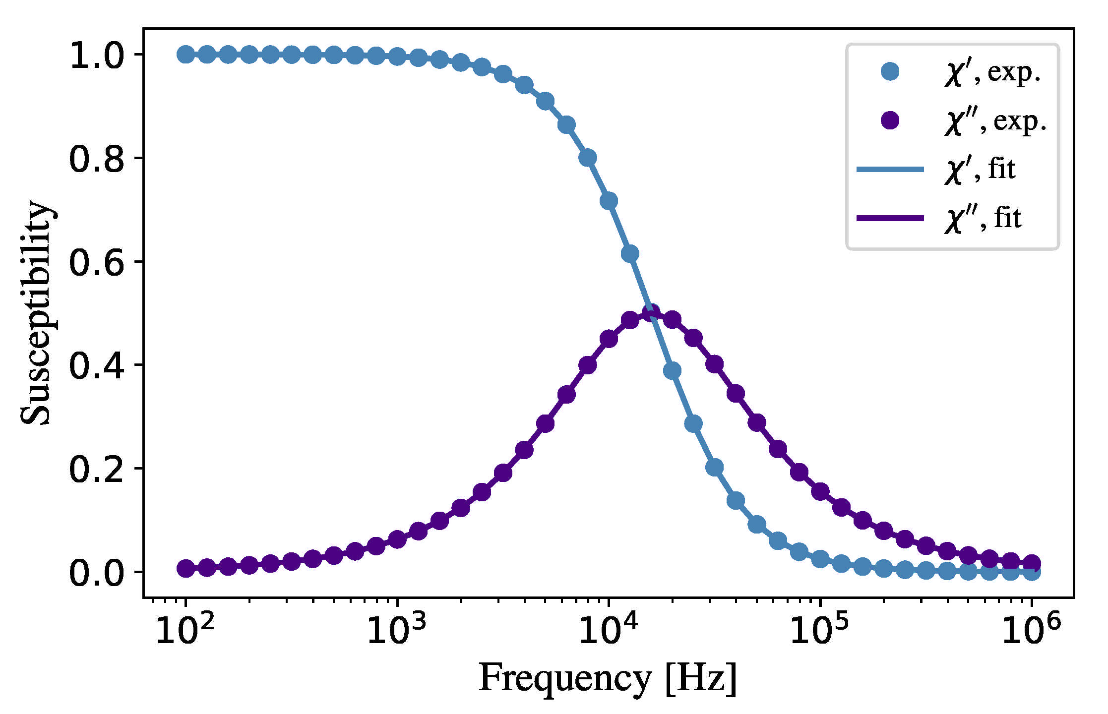
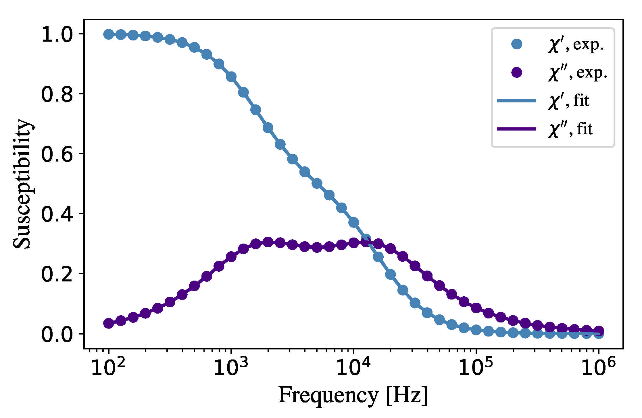
• We use the obtained numeric dataset of experimental points for the real, ${\chi }_j^{\prime }$, and the imaginary, ${\chi }_j^{″}$, susceptibilities. We count these data with sign $j\in [1,M]$, where M stands for the total number of experimentally measured susceptibilities at the frequencies $f_j$. The static Langevin susceptibility ${\chi }_{\mathrm{L}}$ is determined as the zero-frequency limit of ${\chi }_j^{\prime }$ on the basis of static MW susceptibility (6), ${\chi }_{\mathrm{MW}}^{\prime }\left(0\right)={\chi }_{\mathrm{L}}\left(1+\frac{1}{3}{\chi }_{\mathrm{L}}\right)$.
• To reduce the number of unknown parameters for the optimization and to minimize the computation time, we fix the set of the fraction relaxation times ${\tau }_k$ being distributed evenly at the logarithmic scale, for example, ${\tau }_k={10}^{-k}\mathrm{s},k=\in [1,N]$. Importantly, the number of fractions does not exceed ten, $N\le 10$. The amplitudes $A_k$ are to be determined numerically from the condition

  $$\sum _{j=1}^M\left\{R\left(\frac{{\left[{\chi }_{\mathrm{MW}}^{\prime }\left(f_j\right)-{\chi }_j^{\prime }\right]}^2}{\left|\right|{\chi }^{\prime }\left|\right|}\right)+R\left(\frac{{\left[{\chi }_{\mathrm{MW}}^{″}\left(f_j\right)-{\chi }_j^{″}\right]}^2}{\left|\right|{\chi }^{″}\left|\right|}\right)\right\}\to min,$$

  (8)

  where $\left|\right|\chi \left|\right|=max|{\chi }_j|$. Function $R\left(z\right)$ can be any monotonously increasing sub-linear function of its variable z, given in criterion (8) in round brackets; we use here the function $R\left(z\right)\equiv ln(1+z)$. Such a choice prevents a situation when the least-squares solution can become significantly biased to avoid very high residuals on outliers [20]. We insert the denominators in the functional (8) in order to equalize the contributions from the real and the imaginary parts of the dynamic susceptibility. The number of fitting parameters $A_k$ is equal to N, and it is not too much; the numerical optimization is very fast, and the optimization results are not affected by the experimental fluctuations.
  The optimization condition (8) includes summation over index j from 1 to M, so the total number of experimental data is used during the fitting for both susceptibilities,${\chi }_j^{\prime }$ and ${\chi }_j^{″}$. So, the algorithm requires the best coincidence between theory and experiment simultaneously for both susceptibilities.
• With this first numerical fitting we get the N points at the plane $(\tau ;A)$, which describes roughly the relaxation time spectrum for MNP fractions. Of course, there are not many of these points, and they are well separated from each other. An example is given in

  Table 1. Example of the set of fraction relaxation times. The number of fractions N is 6. The fitting time interval is from ${10}^{-7}\mathrm{s}$ to ${10}^{-1}\mathrm{s}$. The time shift $\delta$ is 0.2. The number of fits is 5. So we get 30 points in the plane $(\tau ;A)$ to characterize the time relaxation spectrum.

  Fit	$lg{\mathit{\tau }}_6$	$lg{\mathit{\tau }}_5$	$lg{\mathit{\tau }}_4$	$lg{\mathit{\tau }}_3$	$lg{\mathit{\tau }}_2$	$lg{\mathit{\tau }}_1$
  1	−7	−6	−5	−4	−3	−2
  2	−6.8	−5.8	−4.8	−3.8	−2.8	−1.8
  3	−6.6	−5.6	−4.6	−3.6	−2.6	−1.6
  4	−6.4	−5.4	−4.4	−3.4	−2.4	−1.4
  5	−6.2	−5.2	−4.2	−3.2	−2.2	−1.2

  . Then, we shift the set ${\tau }_k$ with some $\delta$, which fits an integer number of times in an interval: $lg{\tau }_k-lg{\tau }_{k+1}=m\delta ,m\in \mathrm{N}$. For the previous example ${\tau }_k={10}^{-k}\mathrm{s},k=\in [1,N]$, $\delta$ might be 0.1 and $m=10$. So, the next set of fractions are characterized with the relaxation times, each of them is shifted with $+\delta$ in the logarithmic sale in comparison with the previous set of fraction relaxation times, but the number of fraction N remains the same. To explain this point in more details we show Table 1 as an example when the number of fractions is chosen as 6. The first set of fractions is given in the first line “Fit 1”. The second set of fractions is presented in line “Fit 2”, and the relaxation times here are shifted with $+0.2$ in the logarithmic scale. Then, we shift the fractions again and again, $m-1$ times, and for each case we apply the numerical optimization of criterion (8) for each new set of fractions independently of previous fittings, and we determine the amplitudes. After that we combine all fitted parameters together and normalize the amplitudes according to normalization condition (4), and so we get the $mN$ number of points at the plane $(\tau ;A)$.
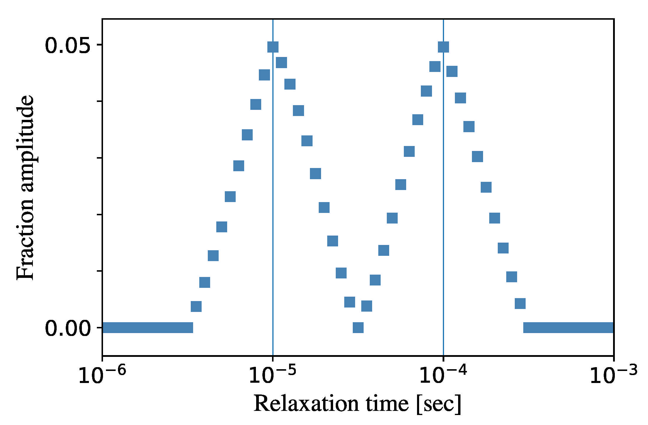
• For real ferrofluids the MNP relaxation times range from ${10}^{-9}\mathrm{s}$ (the Néel superparamagnetic relaxation) to ${10}^{-1}\mathrm{s}$ (the Brownian relaxation), depending on the MNP size. Testing of the described algorithm in this time range reveals that the stable and low-noisy fitting results can be obtained even for rather small number of fitting fractions: $6\le N\le 10$. The PC computation time takes no more than several seconds, and it increases with N according to parabolic law: $\propto N^2$.
• The advantages of this algorithm are: (i) it converges rapidly for each numerical realization for N fractions; (ii) we get the numerical fitting with m-times larger number of fractions than N; (iii) we get the ’smooth’ fitting because a small number of fractions N at each realization means that we average over the MNP contributions inside some interval of the relaxation times, so we avoid the influence of experimental errors. The resulting array of points $A_i\left({\tau }_i\right),i\in [1;mN]$ should be considered as the desired spectrum of the MNP relaxation times.

2.3. Program Implementation

To perform the actual fit, the target function (8) is minimized using the differential evolution algorithm, which was first introduced in Ref. [21]. Differential evolution method belongs to a class of stochastic methods: it does not compute a gradient of function, and this method is quite similar to the Monte–Carlo technique, widely used in computer simulations. Differential evolution actually is not a single method, but it is a wide group of similar algorithms that differ in details. Here, we use the implementation code available in the scientific Python library [22]. Visualisation of the results was obtained also with the help of Python library [23].

It is well-known [24] that the convergence of the differential evolution algorithm strongly depends on its parameters. In our case, the default parameters of the library [22] appeared to be suitable. More precisely, the differential evolution strategy was “best/1/bin” according to almost standard nomenclature used in the literature [25]. The maximum number of generations (over which the entire population is evolved) was chosen to 20,000. The population had $15\ast N$ individuals. The mutation constant was taken from $[0.5,1)$ because dithering was employed. In the literature mutation constant is also known as differential weight, being denoted by F. The recombination constant, which is also known as the crossover probability, was equal to 0.7. Type of population initialization corresponded to the Latin Hypercube sampling which tries to maximize coverage of the available parameter space. The best solution vector was continuously updated within a single generation [26]. The domain of unknowns amplitudes $A_k$ was limited by a segment $[0;1]$.

Obviously, our target function (8) satisfies the Lipschitz condition. This means that more complicated numerical algorithms might be used guaranteeing the global convergence. Construction of the algorithm, described here in Section 2.2, allows us to use almost any modern optimization method due to the fact that our method requires for the fitting with the quite small number N of MNP fractions.

3. Results

To test the suggested numerical algorithm and to show its efficiency we performed two computer experiments for the most difficult cases when the particle size distribution of the studied ferrofluid is very narrow and close to the delta-function. In the first experiment (A) the mono-fraction ferrofluid is studied, and the MNP relaxation time is considered as ${10}^{-5}\mathrm{s}$. The second experiment (B) is performed for bi-fraction ferrofluid, the relaxation times of fractions are ${10}^{-5}\mathrm{s}$ and ${10}^{-4}\mathrm{s}$, the amplitudes of both fractions are equal to 0.5. The Langevin susceptibility is ${\chi }_{\mathrm{L}}=1$ for both ferrofluids A and B, and we neglect the interparticle interaction for simplicity.

The frequency spectra of the initial dynamic susceptibility were calculated with the help of expressions (1) and (2). We consider the obtained dataset of dynamic susceptibilities as the experimental data, and we indicate these data as the experimental dots in Figure 1 and Figure 2. These spectra were fitted according to the described numerical algorithm with varying number of fractions from 6 to 9.

Dependencies of both parts of the ferrofluid A dynamic susceptibility on the frequency f of AC probing field are shown in Figure 1. The spectrum is a pure Debye-like one, and the imaginary part demonstrates the maximum at the frequency ${10}^5/2\pi \approx 1.6\times {10}^4\mathrm{Hz}$. The same frequency spectrum for the ferrofluid B is shown in Figure 2. Here, we see two imaginary susceptibility maximums produced by two fractions. Since the amplitudes of both fractions are equal and the interparticle effects are not taken into account, the heights of both maximums are also coincident. The results of fitting are presented with curves, and the numerical errors are invisible.

Theoretical curves in Figure 1 and Figure 2 were calculated on the basis of the presented algorithm (Section 2.2), and the amplitudes of the fractions were determined within the optimization of criterion (8). The results for the spectra are presented in Figure 3 and Figure 4 in the plane “fraction relaxation time—fraction amplitudes”. We would only like to mention here that for both ferrofluids, A and B, the agreement between ’experimental’ dots and the theoretical curves is perfect.

The obtained spectrum of the relaxation times for ferrofluid A is presented in Figure 3, and since we are trying to reconstruct the delta-function distribution, we show here the results of fitting algorithm with different number of fitting fractions. We see the peak both in Figure 3a,b, the maximum of which coincides with the relaxation time ${10}^{-5}\mathrm{s}$, which was put into the model mono-fraction ferrofluid A. Simultaneously, the following tendency holds true: the more fractions are used, the narrower is the maximum. Since the set of amplitudes is normalized to unity, the height of the amplitude peak is higher in the case when the larger number of fractions is used in the algorithm.

The obtained spectrum of the relaxation times, obtained for the bi-fraction ferrofluid B, is shown in Figure 4 for the fitting procedure with nine fractions. Evidently, both fractions are checked correctly and the fraction relaxation times ${10}^{-5}\mathrm{s}$ and ${10}^{-4}\mathrm{s}$ are clearly seen. It is worth mentioning that the presented algorithm does not only detect correctly the relaxation times of fractions, but it gives the correct mutual correspondence between the fractions in dynamic susceptibility. We mean here that the fraction amplitudes, found for the bi-fraction ferrofluid B, appear to be coincident, and the peaks in Figure 4 look the same but shifted in one decimal order.

4. Discussion

The relaxation time distribution spectra, obtained in this way, provide the basis for predicting the time response of MNP suspension under the influence of the AC magnetic field. The next step is the characterization of MNPs with their sizes. The transition from time distribution to size distribution requires the one-to-one correspondence between the MNP size and the MNP relaxation time. Traditionally, two physical mechanisms are discussed allowing for rotation of the MNP magnetic moment. The first one is the Brownian thermal motion, when the MNP rotates as a rigid sphere with frozen magnetic moments. The characteristic Brownian relaxation time is proportional to the hydrodynamic volume of the MNP and is linearly dependent on a liquid viscosity [1]. Typically, the range of time of Brownian relaxation mechanism is more than ${10}^{-5}\mathrm{s}$. The second mechanism is connected with the stochastic reorientations of the magnetic moment inside MNP due to thermal fluctuations. This behaviour is known as Néel ’superparamagnetism’, and it is characteristic of nanosized particles only. Superparamagnetic fluctuations are commonly described as the thermally activated rotations of the magnetic moment inside the MNP magnetic core. The characteristic Néel relaxation time depends on the magnetic anisotropy energy [1], which is proportional to the MNP magnetic core volume. Since the magnetic anisotropy of the MNP magnetic material prevents the magnetic moment reorientation, the mentioned dependence is sharply increasing function, but the exact analytical expression is unknown. It is commonly accepted that ferroparticle relaxation with times less than ${10}^{-5}\mathrm{s}$ corresponds to the Néel mechanism. In both cases the relaxation time depends on the additional parameters, like the liquid viscosity and/or the MNP magnetic anisotropy constant, the presence of which make it difficult to construct an unambiguous correspondence between MNP relaxation time and MNP size.

It is worth mentioning that the total range of the relaxation times, fixed in the dynamic susceptibility measurements, is very wide, eight-nine orders of magnitudes, typically from ${10}^{-9}\mathrm{s}$ up to ${10}^{-1}\mathrm{s}$. Evidently, the numerical granulometric algorithm with a finite number of fractions cannot cover this range with sufficient density, for example, at random distribution of the fraction relaxation times. Within our algorithm, we put manually the relaxation times equally dense at the logarithmic time scale. After several shifts, described in Section 2.2, we get the relaxation time spectra with rather large number of points distributed uniformly close to each other, see Figure 3 and Figure 4. In terms of computational time the last point means the main novelty of the algorithm; it is fast; it does not require for huge computational resources, but results in a very broad and rather dense relaxation time spectrum.

In conclusion, our mathematical model results in the simple and fast numerical algorithm for the MNP dynamic magnetic susceptibility, which can be effectively used for processing experimental data and estimating the magnetic characteristics and the relaxation time spectra of MNPs and their suspensions. The possibility of the prediction of these characteristics is of major importance for applications of these objects in biomedicine and modern technologies.

References

1. Rosensweig, R.E. Ferrohydrodynamics; Courier Corporation: North Chelmsford, MA, USA, 2013. [Google Scholar]
2. Rubia-Rodríguez, I.; Santana-Otero, A.; Spassov, S.; Tombácz, E.; Johansson, C.; De La Presa, P.; Teran, F.J.; Morales, M.d.P.; Veintemillas-Verdaguer, S.; Thanh, N.T.K.; et al. Whither Magnetic Hyperthermia? A Tentative Roadmap. Materials 2021, 14, 706. [Google Scholar] [CrossRef]
3. Guba, S.; Horvath, B.; Molnar, G.; Szalai, I. A double cell differential thermometric system for specific loss power measurements in magnetic hyperthermia. Measurement 2021, 169, 108652. [Google Scholar] [CrossRef]
4. Kallumadil, M.; Tada, M.; Nakagawa, T.; Abe, M.; Southern, P.; Pankhurst, Q.A. Suitability of commercial colloids for magnetic hyperthermia. J. Magn. Magn. Mater. 2009, 321, 1509–1513. [Google Scholar] [CrossRef]
5. Fatima, H.; Charinpanitkul, T.; Kim, K.S. Fundamentals to Apply Magnetic Nanoparticles for Hyperthermia Therapy. Nanomaterials 2021, 11, 1203. [Google Scholar] [CrossRef]
6. Billings, C.; Langley, M.; Warrington, G.; Mashali, F.; Johnson, J.A. Magnetic Particle Imaging: Current and Future Applications, Magnetic Nanoparticle Synthesis Methods and Safety Measures. Int. J. Mol. Sci. 2021, 22, 7651. [Google Scholar] [CrossRef] [PubMed]
7. Stueber, D.D.; Villanova, J.; Aponte, I.; Xiao, Z.; Colvin, V.L. Magnetic Nanoparticles in Biology and Medicine: Past, Present, and Future Trends. Pharmaceutics 2021, 13, 943. [Google Scholar] [CrossRef] [PubMed]
8. Draack, S.; Ludwig, F.; Schilling, M.; Viereck, T. Dynamic gelation process observed in Cartesian magnetic particle imaging. J. Magn. Magn. Mater. 2021, 522, 167478. [Google Scholar] [CrossRef]
9. Lu, C.; Han, L.; Wang, J.; Wan, J.; Song, G.; Rao, J. Engineering of magnetic nanoparticles as magnetic particle imaging tracers. Chem. Soc. Rev. 2021, 50, 8102–8146. [Google Scholar] [CrossRef] [PubMed]
10. Lakhtina, E.; Pshenichnikov, A. Dispersion of magnetic susceptibility and the microstructure of magnetic fluid. Colloid J. 2006, 68, 294–303. [Google Scholar] [CrossRef]
11. Kharitonskii, P.; Kamzin, A.; Gareev, K.; Valiullin, A.; Vezo, O.; Sergienko, E.; Korolev, D.; Kosterov, A.; Lebedev, S.; Gurylev, A.; et al. Magnetic granulometry and Mössbauer spectroscopy of FemOn–SiO2 colloidal nanoparticles. J. Magn. Magn. Mater. 2018, 461, 30–36. [Google Scholar] [CrossRef]
12. Lysenko, S.N.; Lebedev, A.V.; Astaf’eva, S.A.; Yakusheva, D.E.; Balasoiu, M.; Kuklin, A.I.; Kovalev, Y.S.; Turchenko, V.A. Preparation and magneto-optical behavior of ferrofluids with anisometric particles. Phys. Scr. 2020, 95, 044007. [Google Scholar] [CrossRef]
13. Bender, P.; Balceris, C.; Ludwig, F.; Posth, O.; Bogart, L.K.; Szczerba, W.; Castro, A.; Nilsson, L.; Costo, R.; Gavilán, H.; et al. Distribution functions of magnetic nanoparticles determined by a numerical inversion method. New J. Phys. 2017, 19, 073012. [Google Scholar] [CrossRef] [Green Version]
14. Ivanov, A.O.; Zverev, V.S.; Kantorovich, S.S. Revealing the signature of dipolar interactions in dynamic spectra of polydisperse magnetic nanoparticles. Soft Matter 2016, 12, 3507–3513. [Google Scholar] [CrossRef] [Green Version]
15. Debye, P. Polar Molecules; Chemical Catalog Company: New York, NY, USA, 1929. [Google Scholar]
16. Ivanov, A.O.; Camp, P.J. Theory of the dynamic magnetic susceptibility of ferrofluids. Phys. Rev. E 2018, 98, 050602. [Google Scholar] [CrossRef] [Green Version]
17. Sindt, J.O.; Camp, P.J.; Kantorovich, S.S.; Elfimova, E.A.; Ivanov, A.O. Influence of dipolar interactions on the magnetic susceptibility spectra of ferrofluids. Phys. Rev. E 2016, 93, 063117. [Google Scholar] [CrossRef] [Green Version]
18. Ivanov, A.O.; Kantorovich, S.S.; Zverev, V.S.; Elfimova, E.A.; Lebedev, A.V.; Pshenichnikov, A.F. Temperature-dependent dynamic correlations in suspensions of magnetic nanoparticles in a broad range of concentrations: A combined experimental and theoretical study. Phys. Chem. Chem. Phys. 2016, 18, 18342–18352. [Google Scholar] [CrossRef] [PubMed] [Green Version]
19. Lebedev, A.; Kantorovich, S.; Ivanov, A.; Arefyev, I.; Pshenichnikov, A. Weakening of magnetic response experimentally observed for ferrofluids with strongly interacting magnetic nanoparticles. J. Mol. Liq. 2019, 277, 762–768. [Google Scholar] [CrossRef]
20. Triggs, B.; McLauchlan, P.F.; Hartley, R.I.; Fitzgibbon, A.W. Bundle adjustment—A modern synthesis. In Proceedings of the International Workshop on Vision Algorithms, Corfu, Greece, 20–25 September 1999; pp. 298–372. [Google Scholar]
21. Storn, R.; Price, K. Differential evolution–a simple and efficient heuristic for global optimization over continuous spaces. J. Glob. Optim. 1997, 11, 341–359. [Google Scholar] [CrossRef]
22. Virtanen, P.; Gommers, R.; Oliphant, T.E.; Haberland, M.; Reddy, T.; Cournapeau, D.; Burovski, E.; Peterson, P.; Weckesser, W.; Bright, J.; et al. SciPy 1.0: Fundamental Algorithms for Scientific Computing in Python. Nat. Methods 2020, 17, 261–272. [Google Scholar] [CrossRef] [PubMed] [Green Version]
23. Hunter, J.D. Matplotlib: A 2D graphics environment. Comput. Sci. Eng. 2007, 9, 90–95. [Google Scholar] [CrossRef]
24. Zaharie, D. Critical values for the control parameters of differential evolution algorithms. In Proceedings of the 8th International Conference on Soft Computing (MENDEL), Brno, Czech Republic, 5–7 June 2002; pp. 62–67. [Google Scholar]
25. Jeyakumar, G.; Velayutham, C.S. An empirical comparison of differential evolution variants on different classes of unconstrained global optimization problems. In Proceedings of the 2009 World Congress on Nature & Biologically Inspired Computing (NaBIC), Coimbatore, India, 9–11 December 2009; pp. 866–871. [Google Scholar]
26. Wormington, M.; Panaccione, C.; Matney, K.; Bowen, D.K. Characterization of structures from X-ray scattering data using genetic algorithms. Philos. Trans. R. Soc. Lond. Ser. A Math. Phys. Eng. Sci. 1999, 357, 2827–2848. [Google Scholar] [CrossRef]
Figure 1. Dynamic susceptibility frequency spectrum for the mono-fraction ferrofluid A. The computer experiment dots for both real and imaginary susceptibilities are shown with circles. The curves demonstrate the result of fitting with the help of the presented algorithm with 9 fractions, and the time shift is δ = 0.1 .
Mathematics 09 02450 g001
Figure 2. Dynamic susceptibility frequency spectrum for the bi-fraction ferrofluid B. The computer experiment dots for both real and imaginary susceptibilities are shown with circles. The curves demonstrate the result of fitting with the help of the presented algorithm with 9 fractions, and the time shift is δ = 0.1 .
Mathematics 09 02450 g002
Figure 3. The relaxation time spectrum, obtained for the ferrofluid A, is shown in the plane ’relaxation time—fraction amplitude’, ( τ ; A ). The fraction relaxation time, used in the computer experiment, is 10 5 s . (a) Fitting with 5 fractions and the time shift δ = 0.1 . (b) Fitting with 9 fractions and the time shift δ = 0.2 .
Mathematics 09 02450 g003
Figure 4. The relaxation time spectrum, obtained for the ferrofluid B, is shown in the plane ’relaxation time—fraction amplitude’, ( τ ; A ). The fraction relaxation times, used in the computer experiment, are 10 5 s and 10 4 s . Fitting algorithm was used for 9 fractions and the time shift δ = 0.1 .
Mathematics 09 02450 g004