A Comparative Analysis of Some Methods for Wind Turbine Maximum Power Point Tracking

Abstract

The study in the paper is placed in the broad context of research for increasing the efficiency of capturing and converting wind energy. The purpose of the study is to analyze some mathematical methods for maximum power point tracking in wind turbines. The mathematical methods studied are on–off control, fuzzy control, and neural predictive control. The rules developed for maximum power point tracking are presented. The related control structures and their design methods are presented. The behaviors of the control systems and their energy efficiency are analyzed. Maximum power point tracking ensures a significant increase in the energy generated compared to the unfavorable case of operation at a small and constant load torque. The differences in energy efficiency between the methods of maximum power point tracking studied are small.

1. Introduction

The paper presents the results of a research study in the field of mathematical methods applied to wind energy. The paper includes examples of modeling, control, and optimization in order to increase efficiency in the exploitation of wind energy.

The purpose of the work is the analysis of methods for maximum power point tracking in the operation of wind turbines, taking as a criterion for performance the energy generated. Three methods were chosen, namely: on–off control, fuzzy control, and neural predictive control. The significance of the study is that it shows the efficiency of these methods, compared to each other and compared to the case in which the turbine operates freely.

Several papers are cited, as follows, to show the current state of the literature in the field. The method of the maximum power point tracking is often used in the literature for wind turbine control. Some papers using this method can be mentioned. The paper [1] presents an adaptive algorithm for low energy systems, functioning at turbulent wind. The proposed algorithm combines the computational behavior of hill climb search and power signal feedback control algorithms for tracking of maximum power point. The proposed method from [2] combines hysteresis control with tip speed ratio control using a power coefficient curve. The effectiveness of the proposed algorithm is verified by simulation of a 3 kW wind turbine system. The paper [3] presents a maximum power point tracking system for a small wind turbine connected to a DC micro-grid. The system has a permanent magnet synchronous generator interfaced to the DC micro-grid through a rectifier and a boost converter. The proposed system uses the DC link power and voltage to obtain the required inductor current in the converter to provide maximum power output at all wind speeds. The paper [4] is based on the same power conversion, but it proposed a method that provides a reference current for a proportional integral inductor current controller. Researchers in the field have conducted comparative studies between various technical solutions based on the maximum power point tracking method. In the paper [5], the tip speed ratio and optimal torque methods are analyzed for a 1.5 MW wind turbine model. Their performances are compared through simulation under different wind speed characteristics. A comparative study of different maximum power point tracking methods for a wind energy system based on a permanent magnet synchronous generator is presented in paper [6]. The analyzed techniques are: hill climbing search, optimal torque control, power signal feedback, and fuzzy logic control. The following characteristics are analyzed: the wind system energy efficiency, the response time, the maximum power to be achieved, and the system behavior during the process. The system was simulated under variable wind speed conditions. The authors considered the fuzzy logic control more efficient compared to other algorithms. The results of the study on wind turbine control systems were published as technical reports in universities, including mathematical models and simulations in Matlab/Simulink [7]. Fuzzy logic is a specific mathematical method of artificial intelligence used in wind turbine control with the maximum power point tracking. A comparative analysis between proportional–integral control and fuzzy logic control is made in [8]. The authors considered, based on simulations, that fuzzy control is better, faster, and more accurate. However, the proportional–integral control has a better ration quality/price. The use of neural networks and neuro-fuzzy networks are also common in the literature. Two control methods for maximum power point tracking applied to a wind turbine module system using the permanent magnet synchronous generators (PMSG) in variable speed atmospheric wind conditions are compared in [9]. The control systems, with artificial neural networks and neuro-fuzzy controllers, are modeled, simulated, and analyzed by using Matlab/Simulink software. In the paper [10], a laboratory prototype of a wind system with a permanent magnet synchronous generator, with an artificial neural network for maximum power point tracking, is modeled in a Matlab/Simulink environment. Maximum power point tracking is also used in photovoltaic systems. A review of some technical solutions is presented in [11]. The papers [12,13] review the state-of-the-art available maximum power point tracking algorithms. In [12], the algorithms are classified according to the control variable, namely, with and without sensor, and also based on the technique used to locate the maximum peak. The comparison is made for various speed responses and the capability to achieve the maximum energy yield. The wind energy system was simulated using Matlab/Simulink software. The paper [13] takes into consideration the fact that choosing an exact algorithm for a particular application requires good skills and each algorithm has advantages and disadvantages.

Some controversial and diverging hypotheses are considered. The wind turbine must operate in a certain geographical area. In this area, the wind energy resource must be known. The wind has speeds in a wide range of values. The wind generator system must capture and convert as much energy as possible. For this purpose, we are looking for methods to increase energy efficiency, in order to operate at various wind speeds, following the point of maximum power on the mechanical characteristic of the turbine. However, this maximum power point is an unstable equilibrium point, and the turbine has an infinity of such points. The tendency in the point of maximum power is that the system, once removed from that point, does not return to it. Moreover, any point on the characteristic of mechanical power–speed in which the wind turbine works is an unstable equilibrium point. The tracking methods presented in the literature lead the wind turbine–electric generator system on different state trajectories.

In this paper, a low power turbine is taken into consideration. The paper presents, in Section 2, preliminary information related to wind energy capture, aspects regarding the structure of a wind turbine control system, the mathematical model of the wind turbine, its characteristics, and the definition of the energy performance criterion. The third section presents the tracking methods considered, namely: on–off control with dead band, fuzzy control, and neural predictive control. A set of nine maximum power point tracking rules has been developed and implemented in the on–off control and fuzzy control in a numerical manner. For the fuzzy control method, the fuzzy variables, the rule base, the membership functions, the inference method, and defuzzification method were chosen. For the neural predictive control method, a neural identification of the wind turbine was performed and the neuronal predictive controller was dimensioned. The methods were modeled and simulated in Matlab/Simulink for variable wind speeds. The results that can be obtained with these methods of maximum power point tracking are presented in Section 4. The characteristics obtained by simulations are compared, analyzed, and discussed in Section 5.

The main contribution of the paper can be summarized as a comparative analysis of three maximum power point tracking methods: on–off control, fuzzy control, and neural predictive control, with application in the particular case of a low power wind turbine operating at a variable wind speed. The behaviors of the system for each of these three methods are analyzed. The energy efficiency of these methods is analyzed. The results are compared with those obtained in the case of unfavorable turbine operation at low load torque, without maximum power point tracking. The analyzed methods ensure the production of an energy up to 60% higher than in the case without tracking. The energy differences between the three maximum power point tracking methods are small; they do not exceed 5%.

2. Preliminaries

2.1. General Considerations

In the last years, the production of electricity based on wind energy has developed as part of the so-called renewable energy [14,15]. The wind turbine is a device that converts the kinetic energy of the wind into mechanical energy. Mechanical energy is used to produce electricity. Low-power turbines are used to charge batteries or as auxiliary power sources. High-power turbines are commercial sources of electricity. The wind energy resource available in a given geographical location is described by the physical size of the energy density, which is calculated as the average of the annual energy available per square meter of a turbine propeller. Geographical places are classified according to their energy class into seven energy classes. Class 1 represents places with the lowest density, below 200 W/m². In addition, the class 7 represents the places with the highest density, between 800 and 2000 W/m² [16]. Total wind energy harvesting is practically impossible, because the air taken by the turbine must leave the turbine. In the literature, it is considered that the maximum coefficient of extraction of wind power at a wind turbine is 59% of the total theoretical power. Energy losses in the wind turbine, such as mechanical losses by friction at the turbine shaft, electromagnetic losses at the electric generator, and losses at the electronic power converter, lead to a decrease in energy generated by the wind installation. In the literature, it is considered that, due to these losses, only a third of the wind energy is used.

A horizontal shaft turbine has the following components: propeller, rotor shaft, mechanical coupling, and a braking system. The turbine must be directed in the opposite direction to the wind. High-power turbines have a wind sensor, coupled with a turbine-positioning servomotor. The mechanical coupling has the role of transforming the low speed rotation of the propeller into a higher speed rotational movement, suitable for driving the electric generator, which operates at a speed of hundreds of revolutions per minute. Wind turbines are designed to harness the wind energy that exists at a particular location. This fact requires aerodynamic modeling to determine the optimal tower height, the automatic steering system, number of blades, and blade shape. The turbines used to produce electricity have two or three blades and are driven by computer-controlled motors, which direct them in the wind direction. Some installations operate at constant speed. However, working at variable speeds can increase energy production. Horizontal shaft turbines for the production of commercial electricity were manufactured from 0.6 MW to 7.5 MW [16].

The following rated parameters are taken into consideration: the air density, maximum rotational speed in operation, the extreme wind speed, the maximum rotational speed on a short time, the value of the maximum energy production per year, and the electrical power generator efficiency.

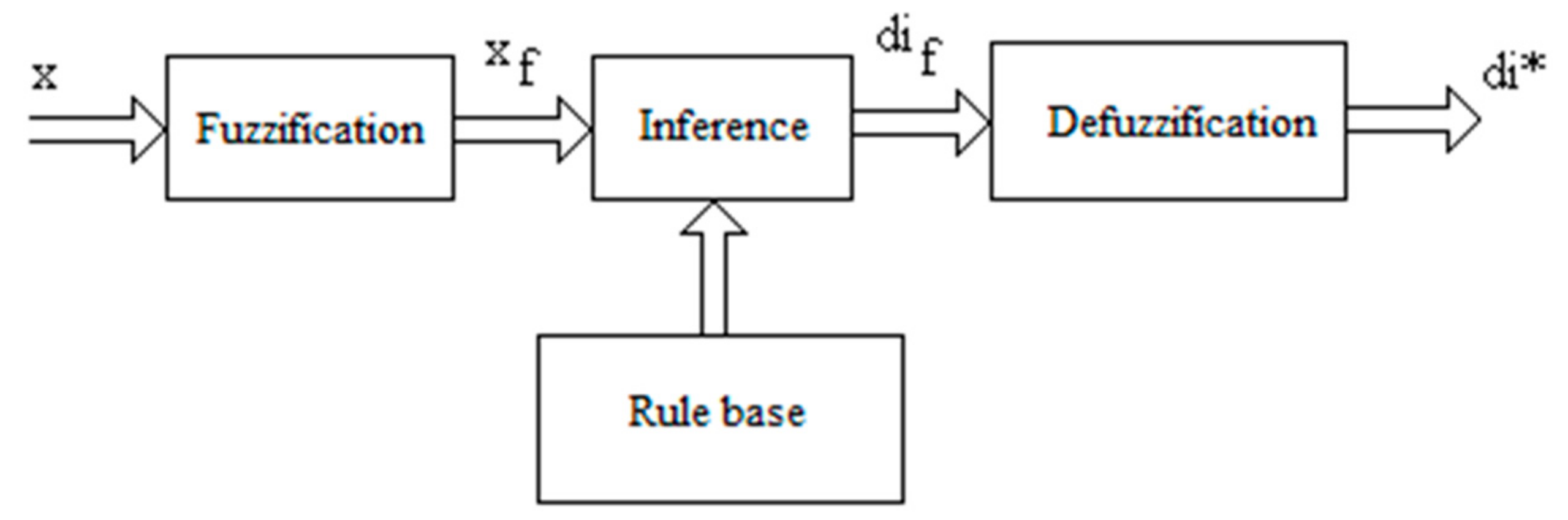
2.2. General Aspects of the Wind Turbine Control Structures

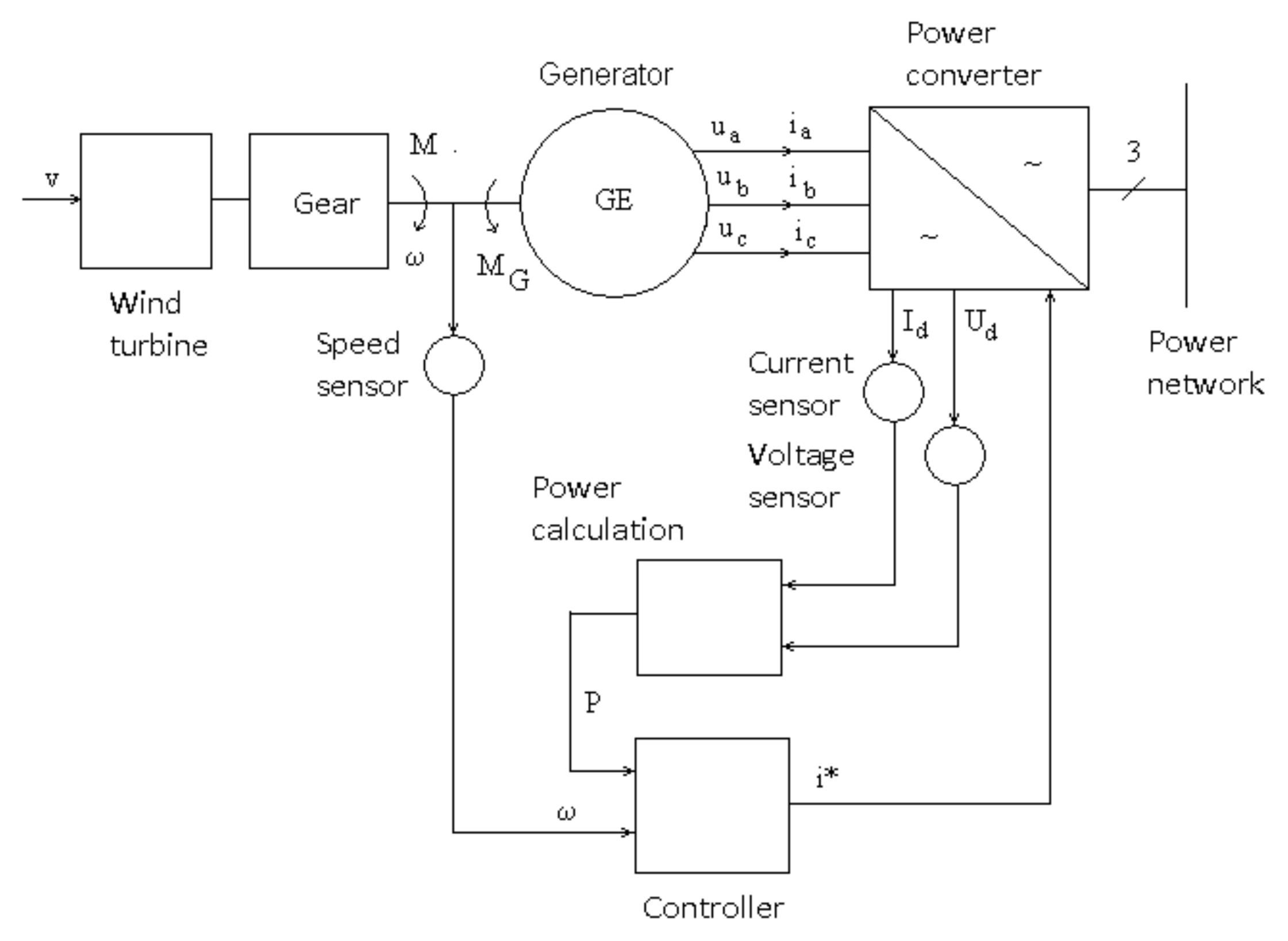
The control structure taken into consideration in this paper, presented in Figure 1, is used on a large scale in wind conversion installations.

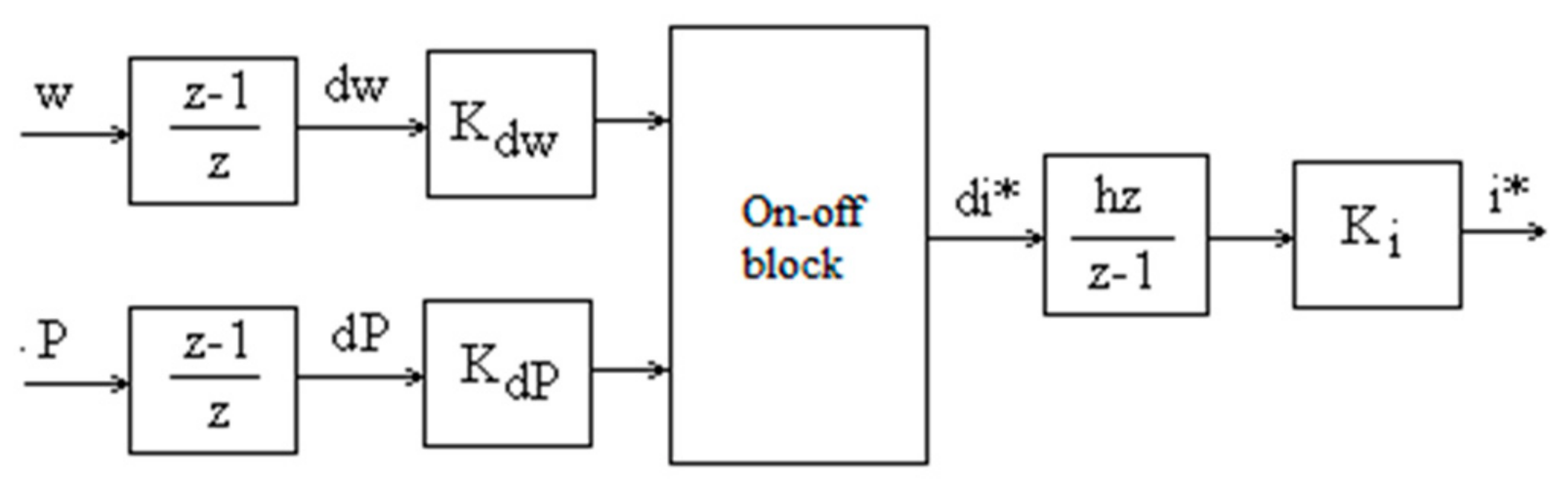
The wind turbine drives through a mechanical gear an electric generator GE, which may be synchronous or asynchronous. The generator supplies the alternating voltages u_a,b,c and currents i_a,b,c. The alternative voltage is converted by a rectifier in direct voltage U_d, which, in turn, is converted to alternative voltage supplied in the network. The current is controlled to the electronic power converter so that the operating point of the turbine is changed. The current controller works based on the information about the speed ω and power P. The speed ω, voltage U_d, and current I_d are measured with sensors. The power is calculated based on the direct voltage and current. The controller sets the current reference i* of the generator load. This is a common control structure, which is used in applications based on maximum power point tracking by adjusting the speed at the turbine axe, controlling the generator with a variable load I_d.

The turbine torque, speed, and power may be adjusted by controlling the I_d current. The controller has two inputs, the speed ω and the power P. Its output is the current reference i*. The control efficiency is determined with a performance criterion, which is the generated energy W.

2.3. Wind Turbine Model

The following relations, well known in the literature, are used in practice for the wind turbine model [14,15,16,17,18].

The mechanical torque M developed by the turbine is given by the relation:

$$M=0.5\pi R^3\rho C_m{v}^2$$

(1)

where R is the radius of the turbine propeller, v is the wind speed, ρ is the air density, and C_m is the torque coefficient, experimentally obtained for a certain wind turbine:

$$C_m=C_{m0}+a\lambda -b{\lambda }^{2,5}$$

(2)

The value:

$$\lambda =\frac{R\mathsf{\omega }}{v}$$

(3)

represents the transmission ratio of the turbine, where ω is the rotational speed of the turbine shaft.

The mechanical power developed by the turbine is calculated with the general relation from the physics of the rotational movement:

$$P=M\mathsf{\omega }$$

(4)

It can be seen that the above relationships are nonlinear.

The simulation parameters of the system are rated power P_n = 5.5 kW; rotation speed ω_r = 12.4 rad/s; the moment of inertia of the wind turbine J_t = 140 kg·m²; the moment of inertia of the electric generator J_g = 1.05 kg·m²; blade swept area A = 19.6 m²; turbine blade radius R = 2.5 m; turbine constants: λ₀ = 3, a = 0.0986, b = 0.0113, C_m0 = 0.0222; specific air density ρ = 1.225 kg/m³. These values are used in the current research performed in the university on an emulator installation of the wind power plant in Seusa, Romania [17,18].

The rated speed ration of the wind turbine λ₀ is a parameter determined with measurements made in an aerodynamic tunnel or on the turbine placement. It is corrected according to experimental measurements. The maximum speed of the turbine is corrected in relation to it.

The following characteristics may be used in practice: the coefficient C_m(λ), as a function of λ; the family of characteristics of the coefficient λ(ω; v); the family of characteristics C_m(ω; v); the family of characteristics of the torque M(ω; v); the family of characteristics of power P(ω; v), from Figure 2, Figure 3, Figure 4, Figure 5 and Figure 6, respectively. All are functions of ω, with v as a parameter. Figure 2, Figure 3, Figure 4, Figure 5 and Figure 6 were obtained by calculations using Equations (1)–(4) and the above numerical parameter values for different wind speeds.

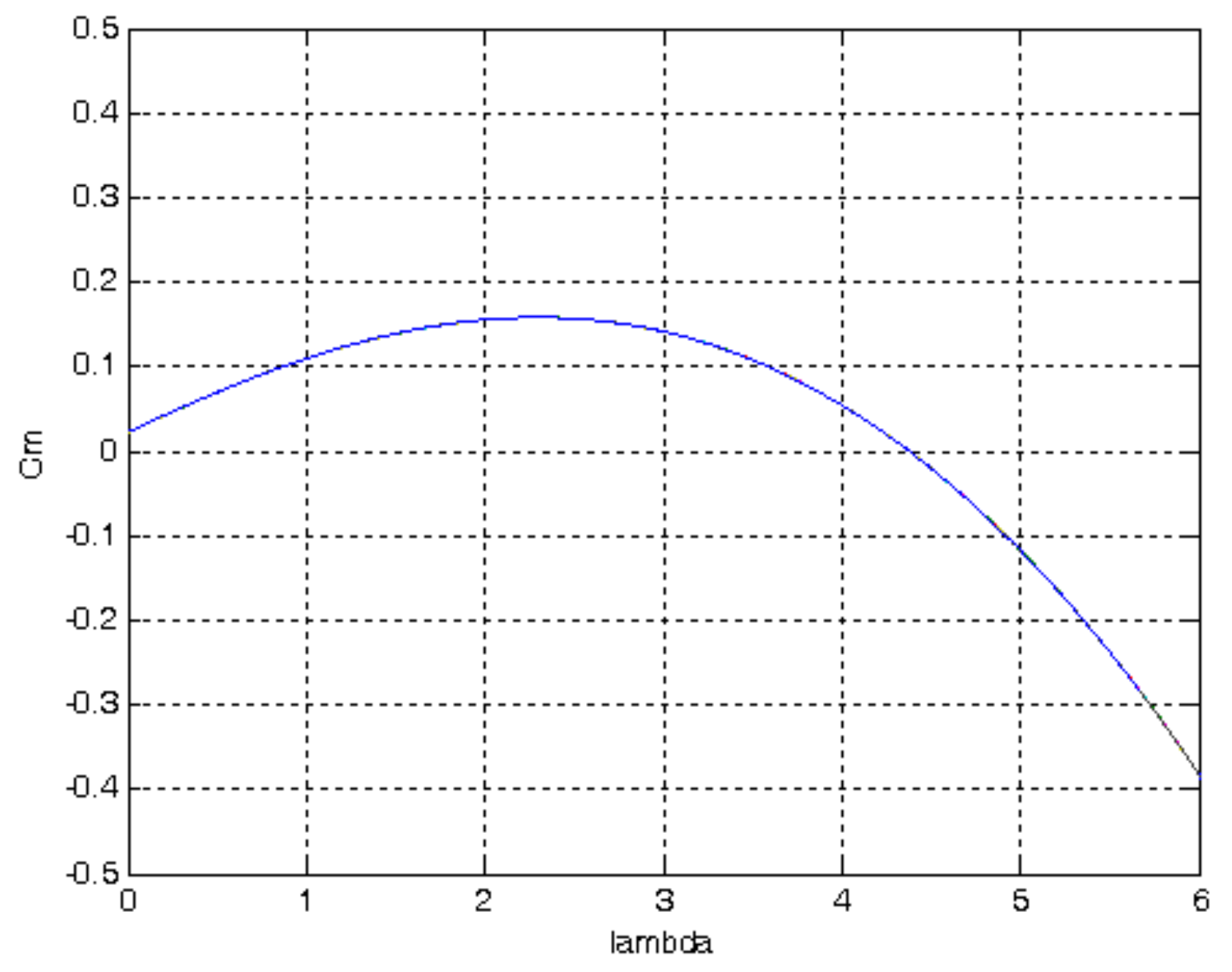
The characteristic of the coefficient C_m(λ) is constant for any value of the wind speed v. The characteristics of the coefficient λ(ω; v) are straight lines, the slope of the straight line is given by the wind speed v, and λ is proportional to the rotational speed ω. The coefficient C_m has a constant maximum value for any wind speed v. The coefficient C_m becomes negative for a ratio λ greater than a specific value. This aspect has a theoretic character. In simulation, for negative values of the coefficient C_m, its value is considered zero. On these characteristics there is a domain (ω, λ) for which λ increases over the maximum value if ω increases or v decreases. If the coefficient λ is less than a specific value of blocking, then the ratio ω/v is less than a specific value. Their variations lead to possible sub-zero decreases in C_m and blockages in the supply of torque and power. 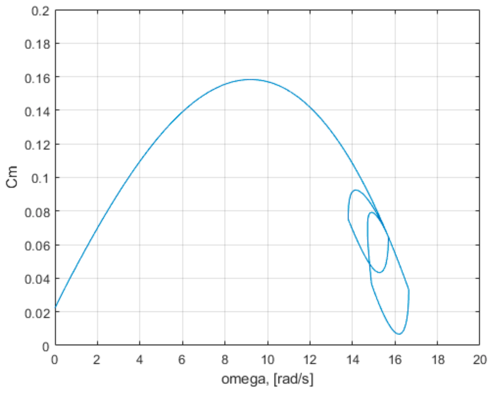High variations under zero C_m, due to decreasing of wind speed or the increasing of the turbine rotation speed, produce jumps and blockages in the supply of torque and power. In Figure 4, it is observed that, for ω = 0, the coefficient C_m has a constant value equal to C_m0 for any value of wind speed. The maximum value of coefficient C_m varies depending on the wind speed. The speed value for which the coefficient C_m becomes negative increases with increasing wind speed. This tells us that the turbine cannot have a high rotational speed if the wind speed is low. 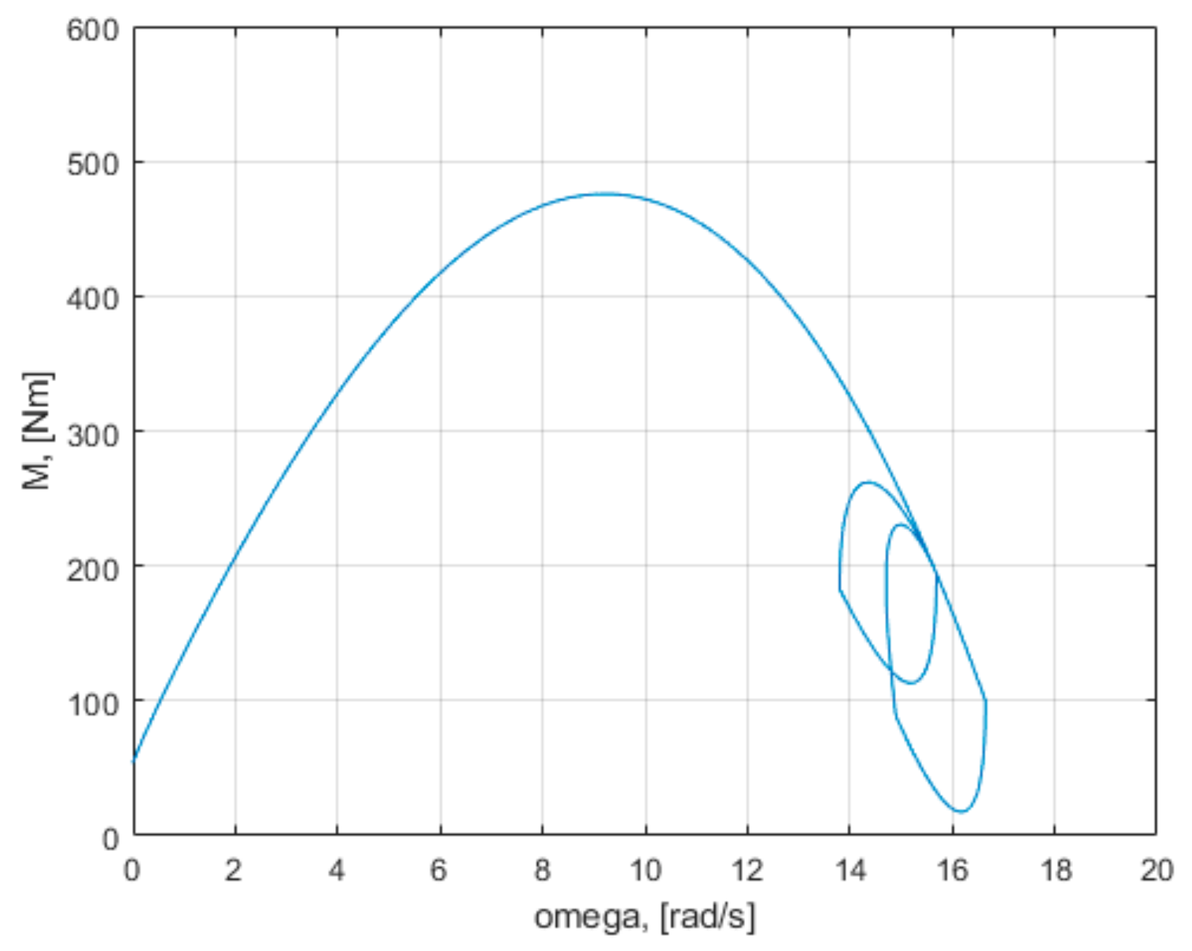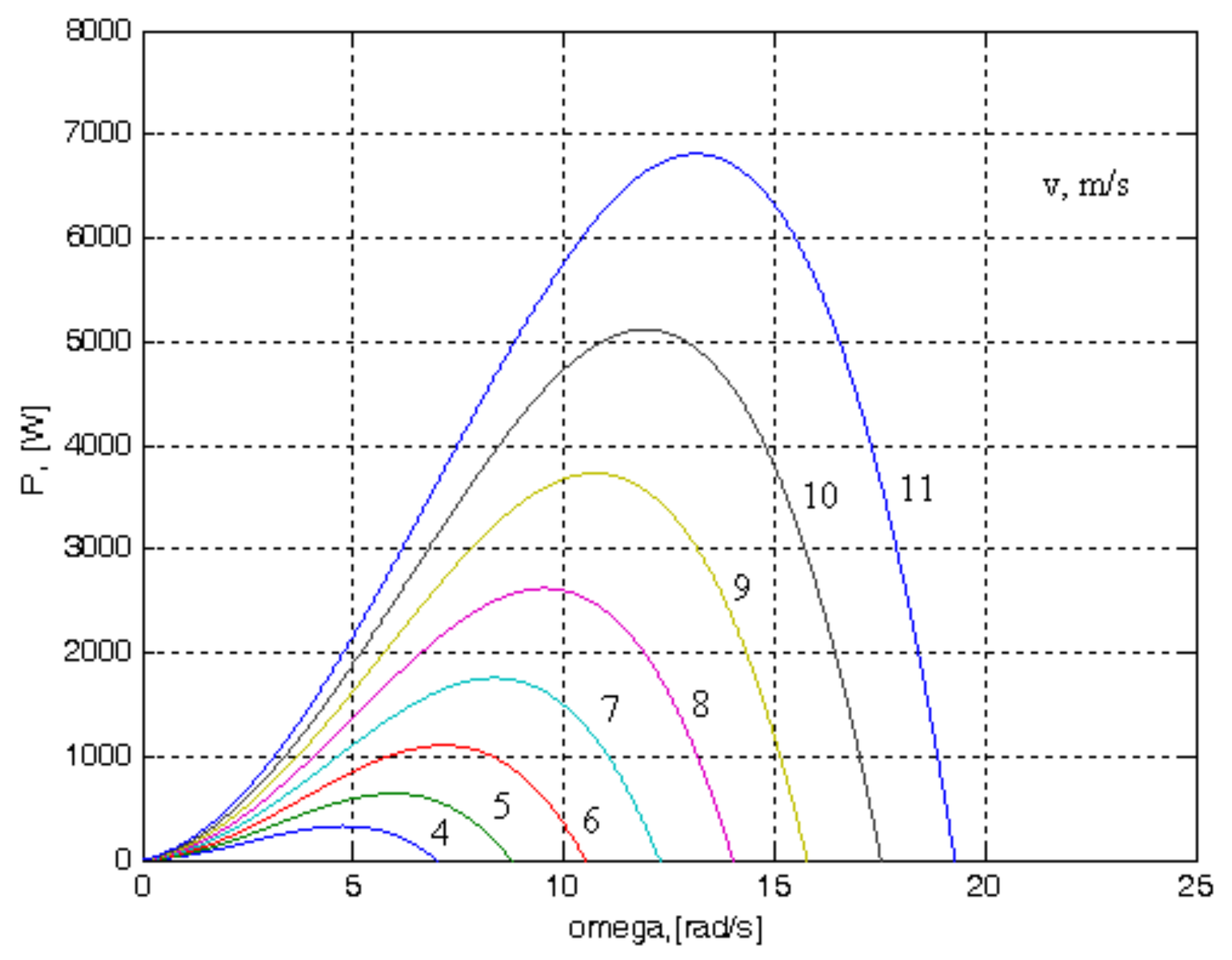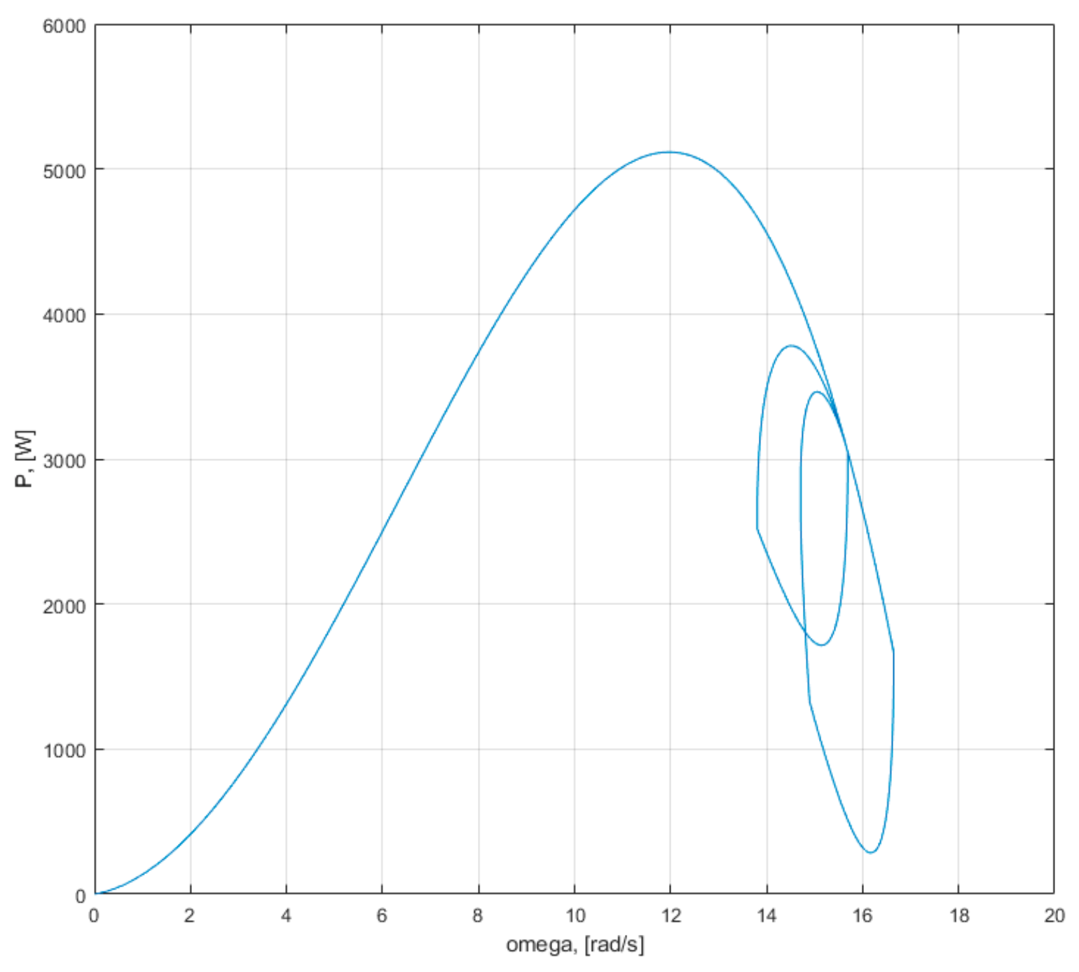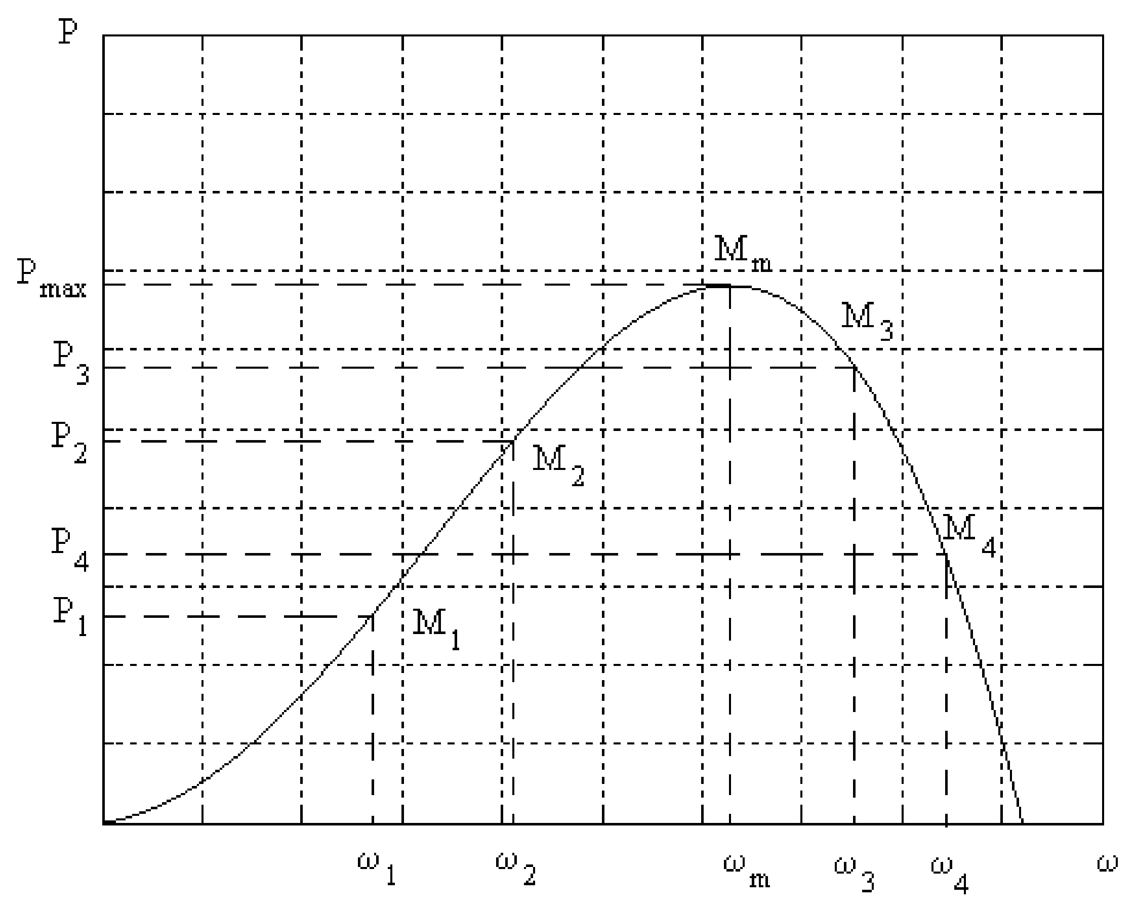It is observed in Figure 6 that the maximum torque, depends on the rotational speed ω and the wind speed v, which is in accordance with the other characteristics. The torque has non-zero values for zero speed at non-zero wind values. The developed torque increases as the wind speed increases, which also allows the rotation speed to increase. It is observed that the maximum power depends on the rotation speed and the wind speed, which is in accordance with the other characteristics. The power has the value zero for zero speed, corresponding to the relation (4). The power developed increases as the wind speed increases, which also allows the speed of rotation to increase.

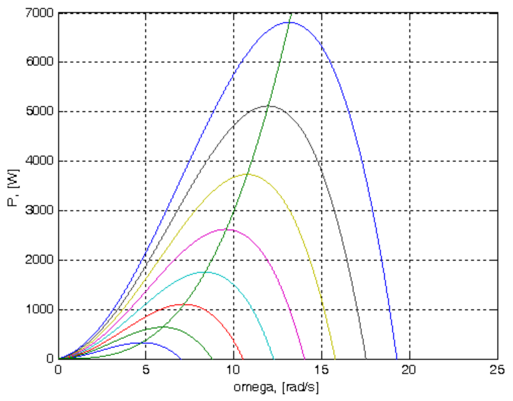
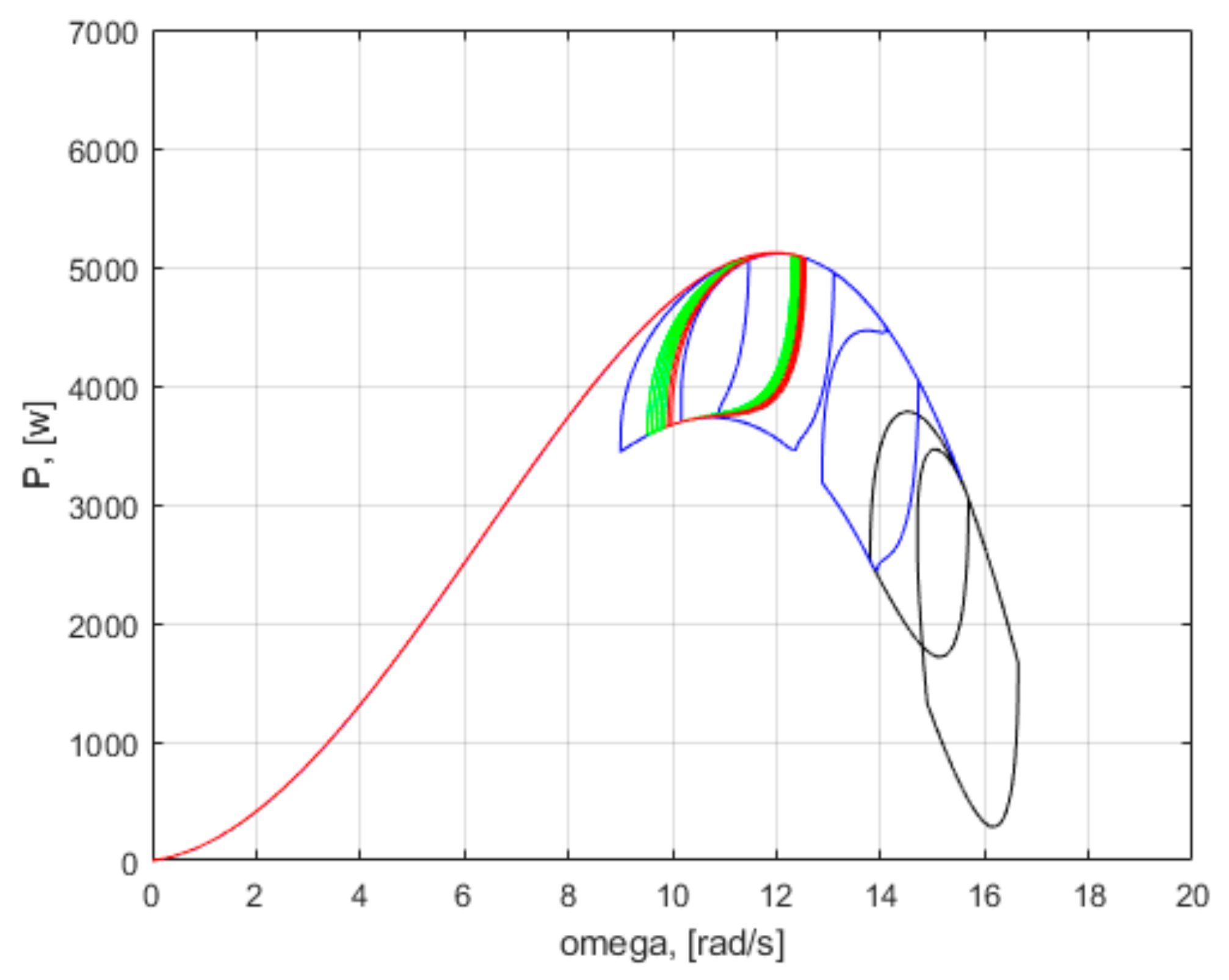
The maximum power on the characteristics of Figure 7 is on a curve:

$$P_m=c_P{\mathsf{\omega }}^3$$

(5)

where c_P = 2.9881 for speed expressed in rad/s and P in Watt.

Figure 7 presents the characteristic of maximum power as a function of speed, superimposed over the characteristics of power–speed. It is observed that this characteristic passes through the maximum points.

Since the speed is related to the wind speed, through relation (3), it can be said that the maximum power also depends on the cube of the wind speed.

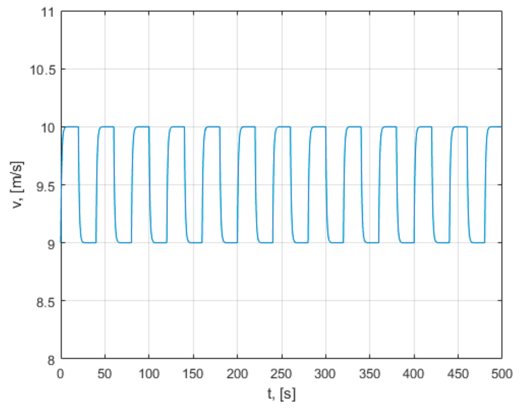
The analysis of the behavior of the wind turbine is done at various wind speeds specific to the geographical location. In the present paper, the analysis of the turbine operation was performed considering a variation in the wind speed from 0 to 10 m/s, and then a periodic change in the wind speed between 9 and 10 m/s, with a period of 40 s, for a duration of 500 s, as in Figure 8.

In the simulation, it was chosen that the variation of the wind speed should not be done suddenly, but with a change after an equation of the first order, with a small time constant of the order of 1 s.

2.4. Dynamic Model of Wind Turbine

The variation of the rotation speed of the turbine shaft is given by Newton’s second law of dynamics:

$$J\frac{d\mathsf{\omega }}{dt}=M-k_f\mathsf{\omega }-M_G$$

(6)

where J is the moment of inertia of the turbine axe, M is the active mechanic torque developed by the turbine, given by the relation (1), k_f is the coefficient of friction at the turbine shaft, ω is the rotational speed of the turbine, and M_G is the load torque introduced by the electric generator. The moment of inertia J is obtained as the sum of the moment of inertia of the turbine J_t and the moment of inertia of the generator J_G:

$$J=J_t+J_G$$

(7)

The coefficient of friction k_f is considered so that the resistive friction torque is 10% of the load torque.

The wind turbine control system has the following variables. The wind speed v is considered as the control input variable. The rotation speed ω and the power P are considered as the output variables. The load torque M_G is a disturbing input variable.

The state Equation (6) is nonlinear, due to the fact that the expression of the active torque and the relations of other variables, given by (1)–(4), are nonlinear.

The wind turbine can be considered as a first-order system:

$$\frac{d\mathsf{\omega }}{dt}=\frac{1}{J}M(v)-\frac{k_f}{J}\mathsf{\omega }-\frac{1}{J}{M}_S$$

(8)

with a high time constant, given by the moment of inertia of the turbine shaft and the coefficient of friction. The rotational speed ω is the state variable.

From the analysis of state Equation (8), it is observed that the rotation speed changes if the rotation acceleration changes:

$$\mathsf{\epsilon }=\frac{d\mathsf{\omega }}{dt}=\frac{1}{J}{M}_{tot}$$

(9)

If the resulting torque M_tot at the shaft increases, then the acceleration increases. If it decreases, the acceleration decreases. The way in which the rotation speed varies affects the operating point of the turbine on the power characteristics P(ω; v), as shown in Figure 6, of the torque M(ω; v), as shown in Figure 5, of the torque coefficient C_m(ω; v), as shown in Figure 4, of the coefficient λ, as shown in Figure 3, and the coefficient C_m(λ), as shown in Figure 2.

Observation: In order to always obtain the maximum power from the power characteristic P(ω; v) from Figure 6 at various wind speeds, the wind turbine must have a rotation speed ω at which this maximum power is obtained. This goal will be pursued in the control strategies adopted in practice.

So, intelligent control rules can be developed based on human reasoning. A negative acceleration ε is required to decrease the rotation speed ω, which, at a constant wind speed v, is obtained by increasing the load torque M_G. In order to increase the rotation speed ω, a positive acceleration ε is required, which, at a constant wind speed v, is obtained by decreasing the load torque M_G.

Equations (1)–(4) and (8) form the mathematical model of the turbine.

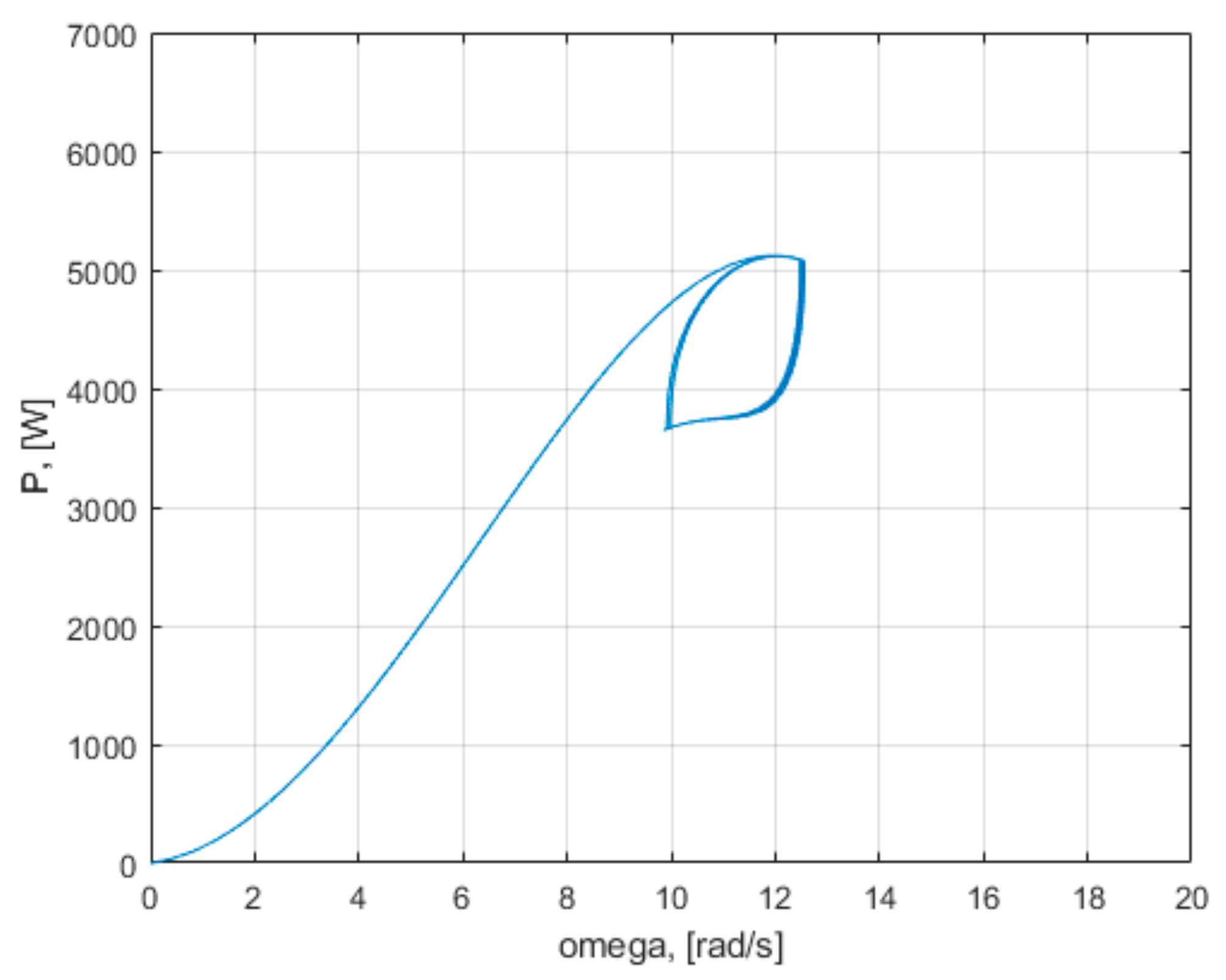
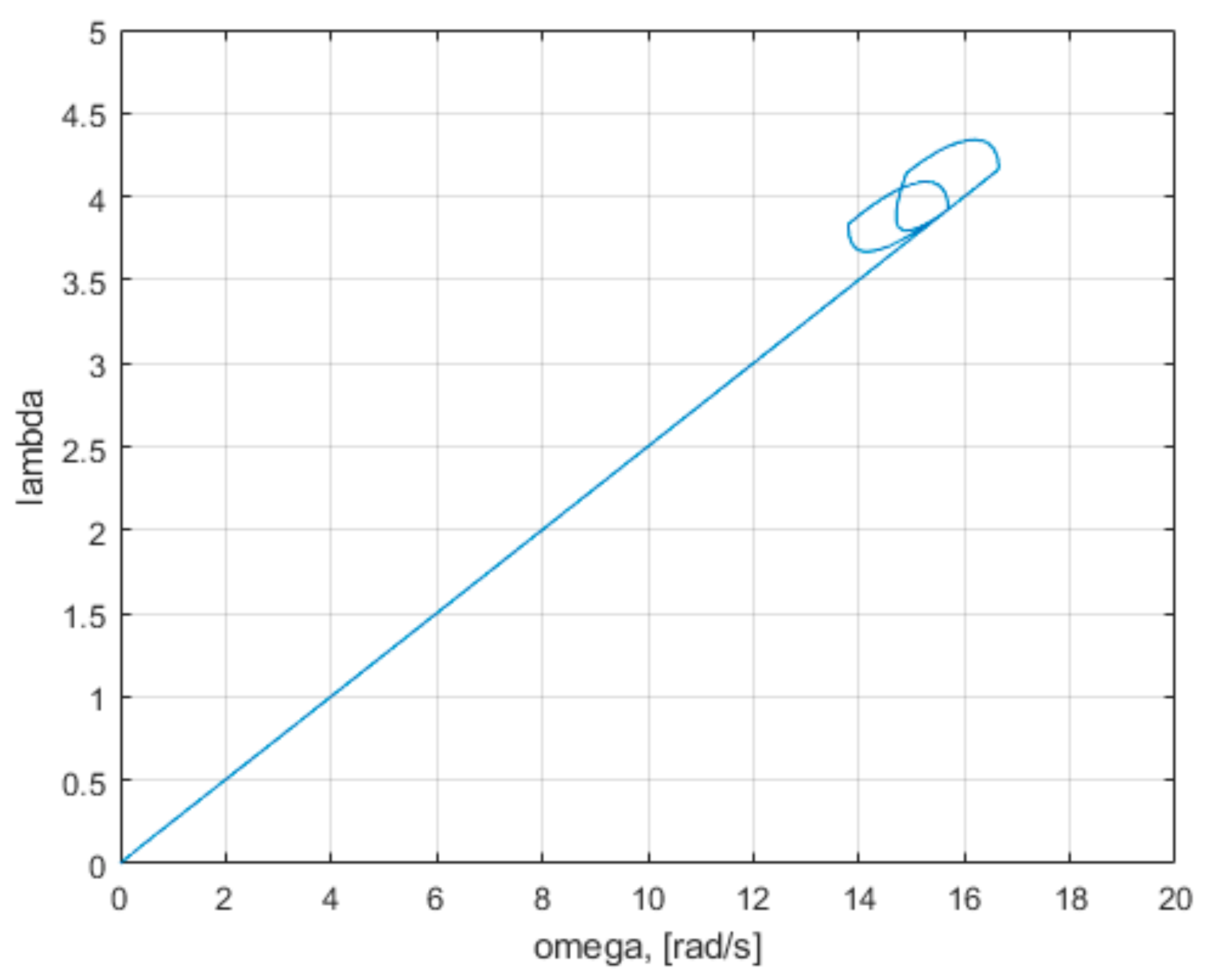
Control methods lead the turbine on various state trajectories, to the maximum power points from the characteristics in Figure 6 for various wind speeds v. The plane of Figure 6 may be considered as a phase plane or a state plane. The geometric representation of the trajectories of the dynamical system in the phase plane may be seen as a phase portrait. Each set of initial conditions is represented by a different curve or point. 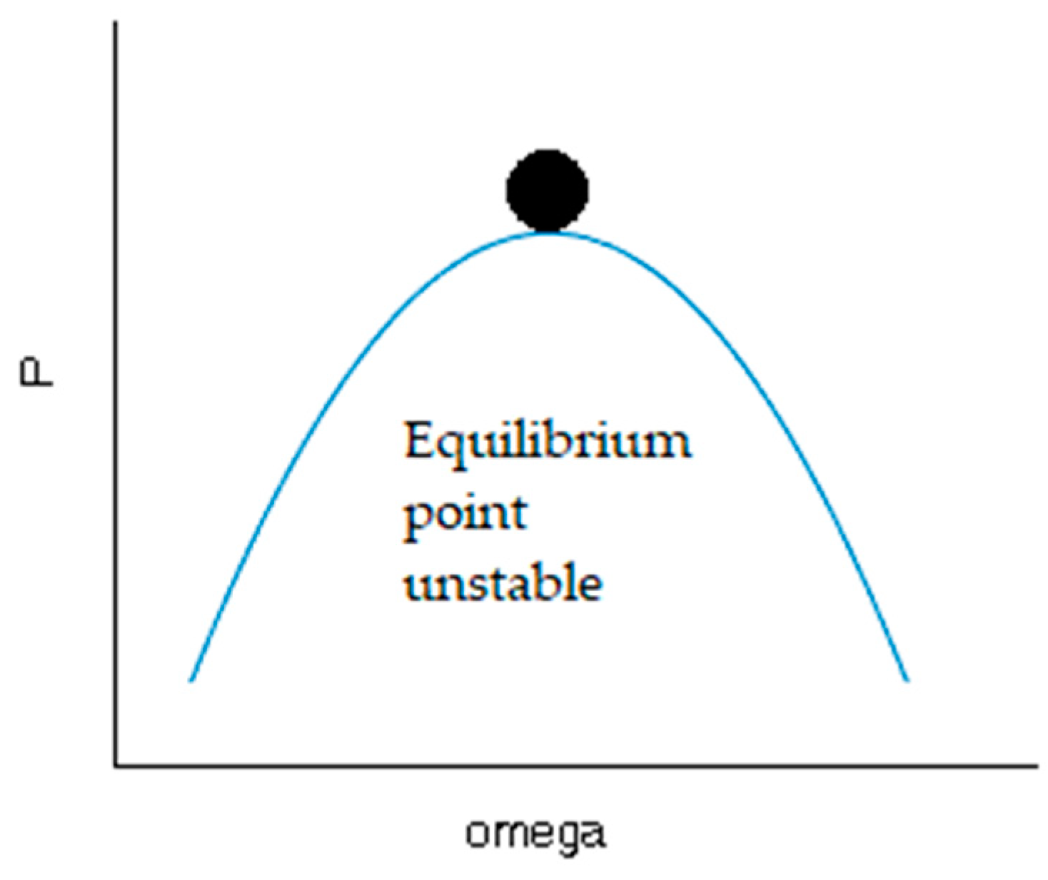The maximum power co-ordinate points (P_max, ω) in the phase plane are equilibrium points. However, these equilibrium points are unstable, according to the classic example from Figure 9.

The turbine has an infinite number of unstable equilibrium points. The main disadvantage of turbine control systems is due to this fact, namely, that it is desired that the operating points of the system be precisely these points of unstable equilibrium. The tendency of the system in the equilibrium point is important, if the system does not return to the equilibrium point, if a small initial condition offset is used, or it is moved away from the equilibrium point. The systems that regulate themselves back to their original operating point when perturbed are normally preferred. In this case, the system does not have this natural tendency, and a feedback control is added to change system behavior from unstable to stable. An analogy can be made between control of a wind turbine and that of a reverse pendulum, namely, in both cases the system is brought to the point of unstable equilibrium. In the literature, there are various mathematical methods of control, which lead the system on various state trajectories and try to keep it in the operating points of maximum power.

Sudden changes in wind speed lead to limit cycles in turbine operation. Limit cycles can reduce the performances of control systems. Oscillations could cause fatigue and damage to mechanical components. Limit cycles may also affect comfort and, ultimately, safety. It is necessary to know if limit cycles occur and to study their stability.

Generator and power converter models are simplified in this study. It is considered that the time constants of the generator and the converter are much smaller than the time constant of the turbine, and they do not influence the regulation. Moreover, in the simulation, the path from regulator to process is considered as a proportional element. Thus, the torque introduced by the generator M_G is proportional to the reference current:

$$M_G=Ki*$$

(10)

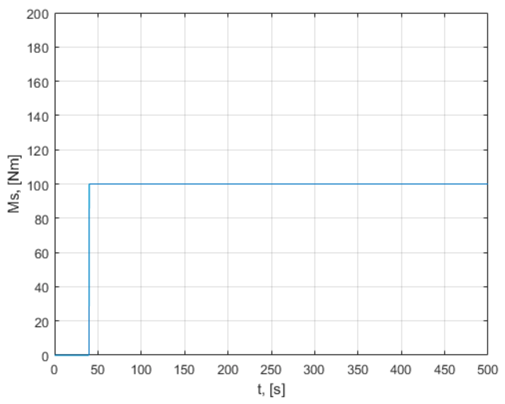
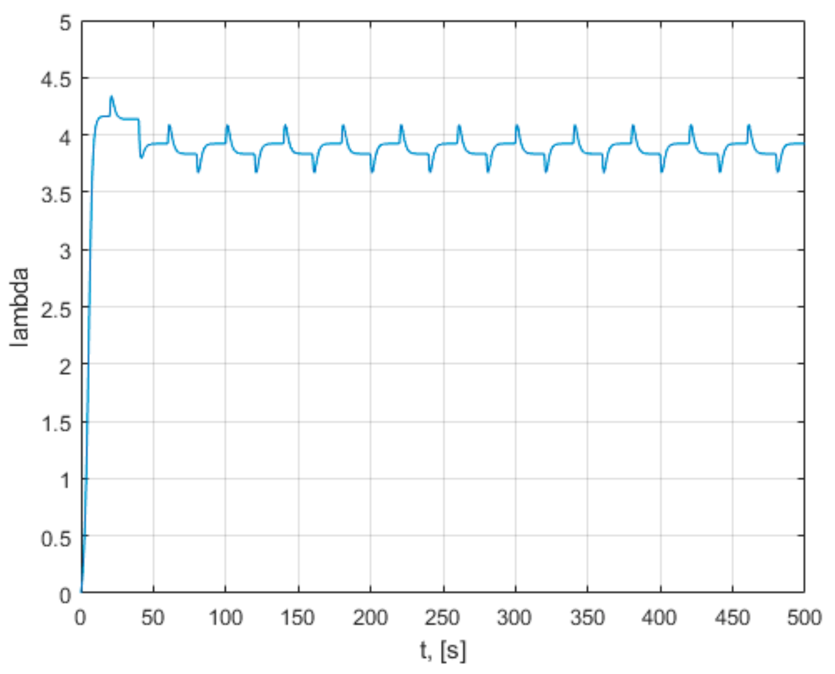
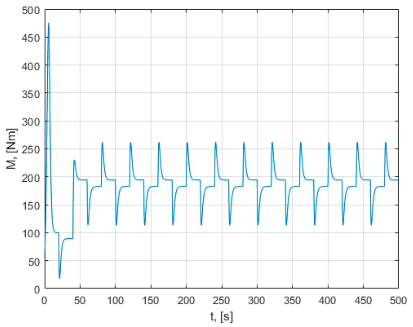
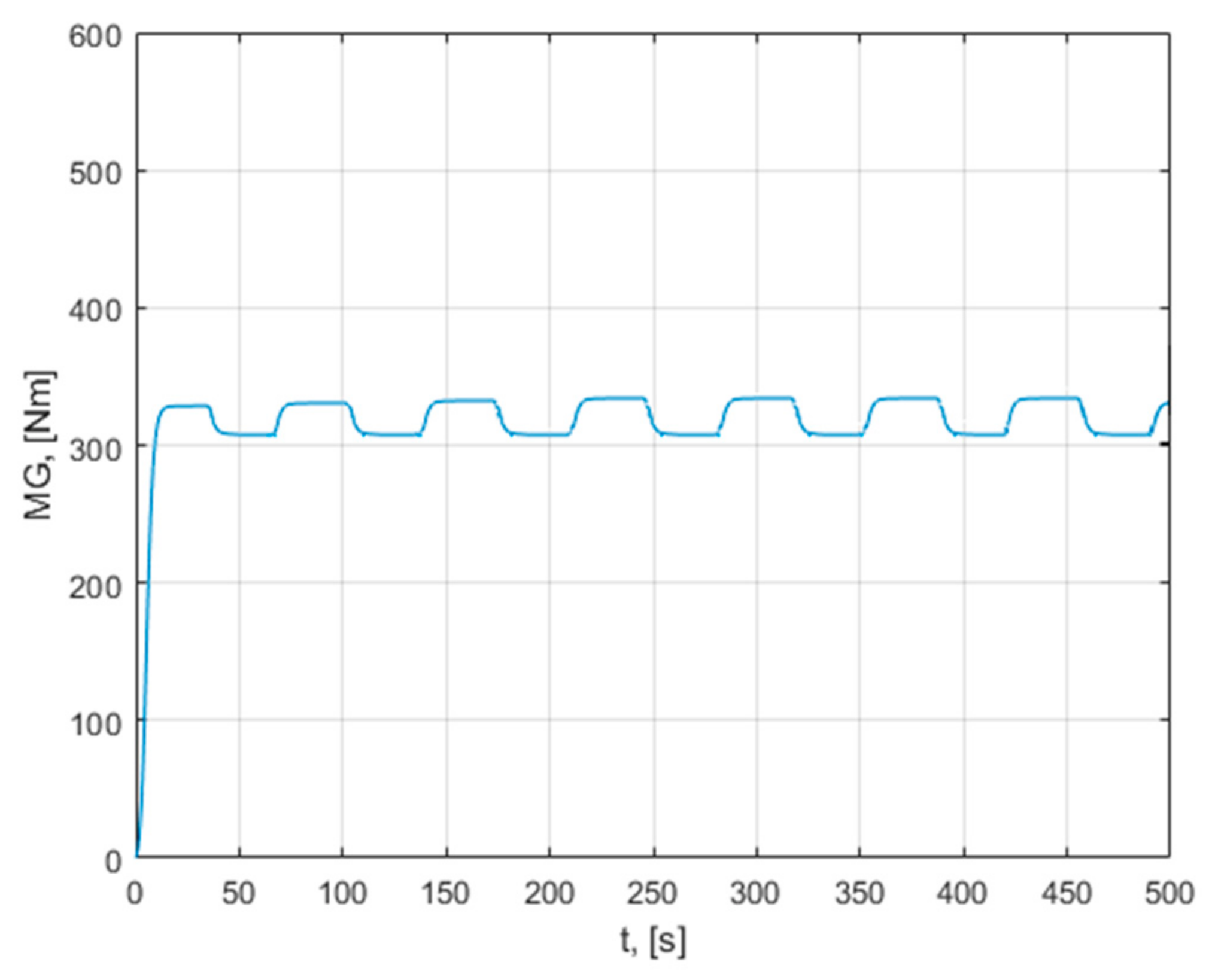
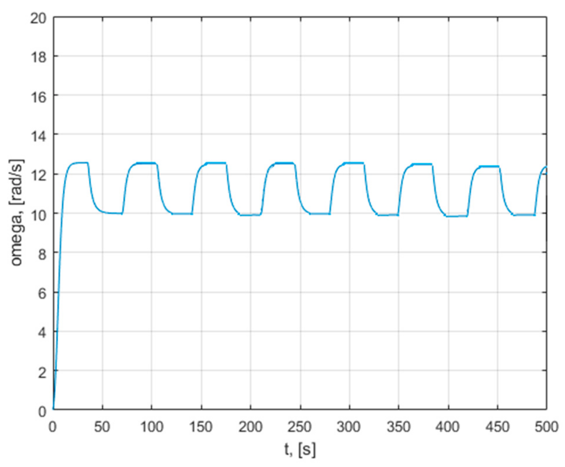
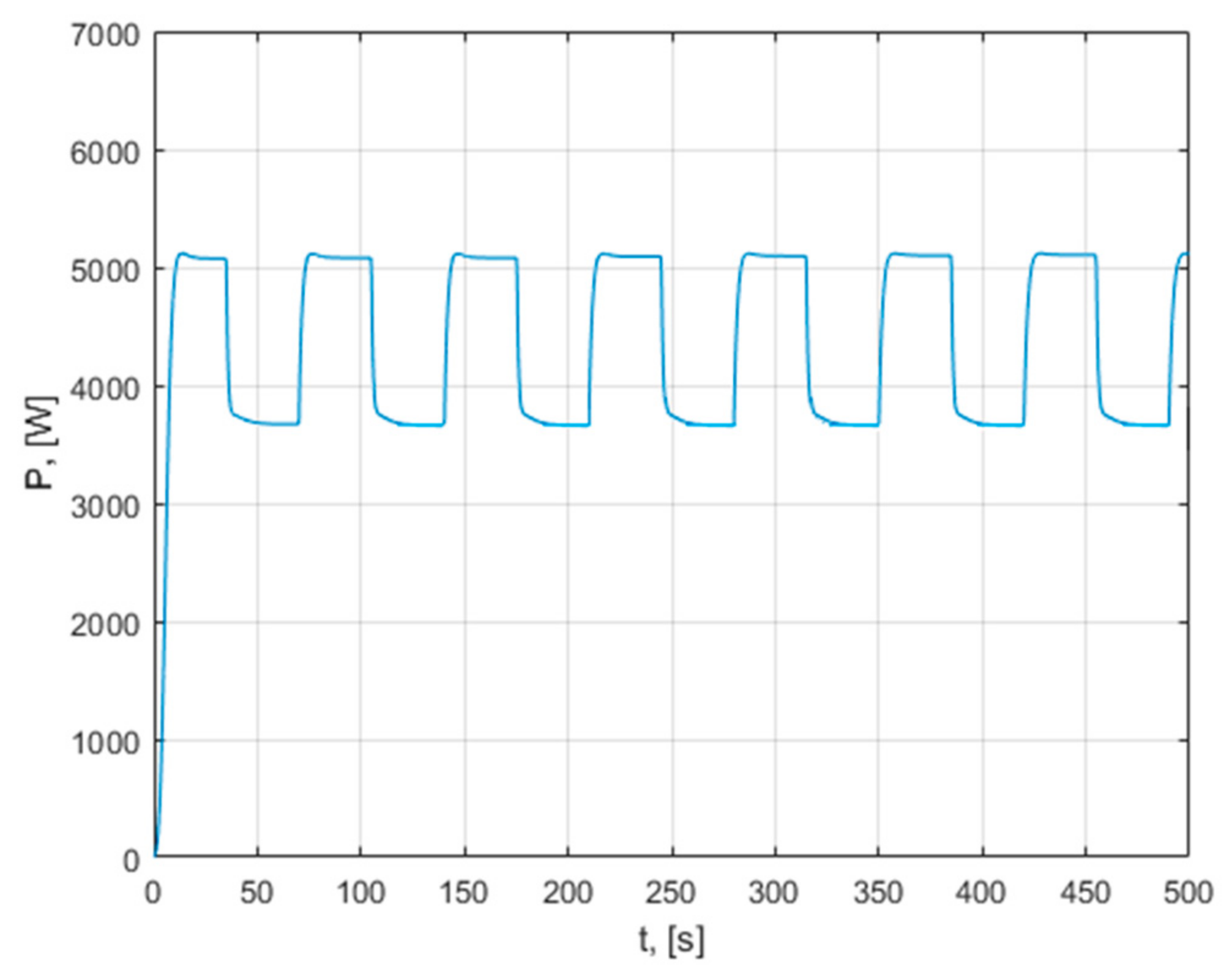
As a basis for comparison for the methods analyzed in the paper, an unfavorable case of operation of the wind turbine is taken. The turbine is considered to be working at high wind speeds, but with a constant, low value load torque. The results of the simulation analysis of this case are presented in Appendix A. As can be seen from those characteristics, the turbine does not reach the maximum power points in the permanent regime, which leads to the need for some maxim power point tracking methods.

2.5. Performance Criterion

The control efficiency study is based on the following performance criterion, which is the energy generated by the system:

$$W={\displaystyle \int P(t)dt\cong {\displaystyle \underset{0}{\overset{tf}{\int }}P(t)dt}}$$

(11)

where P is the developed mechanical power, t_f is the duration of the process analysis, and W is the developed mechanical energy. The electric generator has an efficiency that is maximum at rated power and decreases as the rotational speed decreases. The criterion has the measure unit (kWh), as well the energy. The control performance is better when the value of the criterion, in the same functioning conditions, is higher.

3. Methods

3.1. Maximum Power Point Tracking Method

3.1.1. Functioning Points

Many works that present the method of maximum power point tracking have been published in the literature [1,2,3,4,5,6,12,13]. The maximum power P_max is obtained for different wind speeds v at certain rotational speeds ω, as is presented in Figure 6. So, the maximum power may be reached by controlling the rotational speed of the turbine ω by changing the load power of the electric generator. Figure 10 is used to present the principle of the method. Each power–speed characteristic from Figure 6 has a maximum. Figure 10 presents the principle of tracking for a single power characteristic at a constant wind speed. The functioning point of the wind turbine may be situated on the mechanical characteristic, as in Figure 10: at the left of the point of maximum power M_m(ω_m, P_max), as the points M₁(ω₁, P₁) and M₂(ω₂, P₂), or at the right, as the points M₃(ω₃, P₃) and M₄(ω₄, P₄). The power may increase or decrease around the point of maximum.

3.1.2. Mathematical Condition for Maximum Power

The maximum power requirement can be reached as follows. The power characteristic has the form P = f(ω). The maximum is obtained when the power derivative related to the speed is zero:

$$\frac{dP}{d\mathsf{\omega }}=0$$

(12)

where:

$$\frac{dP}{dt}:\frac{d\mathsf{\omega }}{dt}=0$$

(13)

So, the equivalent condition of maximum may be considered when the maximum of the power derivative related to time is zero:

$$\frac{dP}{dt}=0$$

(14)

3.1.3. The Law of Speed Changing

The law of speed changing can be obtained based on the following reasoning. The modification of the operating point M(ω, P) is done by changing the rotation speed ω. The further to the left or right of the point M_m, the lower the power. The rotation speed change is made according to the second law of dynamics, given by the relation (8). In this relation, it is observed that the variation of the rotation speed in time dω/dt, or the acceleration of the turbine axis, is proportional to the difference between the engine torque developed M and the resistant torque M_G, introduced by the generator, and the inverse proportional to M_G:

$$\frac{d\mathsf{\omega }}{dt}\propto M-M_G\propto -M_G$$

(15)

Turbine torque is proportional to wind speed:

$$M\propto v$$

(16)

The torque of the generator M_G is proportional to the intensity of the current i supplied by the generator:

$$M_G\propto i$$

(17)

So, at constant wind speed and turbine torque, the generator torque M_G and current i must decrease to increase the rotational speed ω. In addition, in order for the rotational speed ω to decrease, the torque of the generator M_G and its current i must increase. Thus, if the generator is loaded with a higher load, its current i increases and the rotation speed ω decreases. In addition, if the generator has a lower load, its current i decreases and the rotation speed ω increases. The rotation speed variation, the acceleration ε = dω/dt, is a quantity inverse proportional to the generator torque M_G or current i. So, the increase in the current i or torque of the generator M_G leads to the decrease in the acceleration ε. If you want to increase the speed, a positive acceleration must be ensured. If a lower rotation speed ω is desired, a negative acceleration ε must be provided. Considering the constant wind speed v, the turbine torque M results are also constant. In addition, the rotation speed change is accomplished only by changing the torque of generator.

3.1.4. Physical Variables

The physical quantities that are taken into account in the driving reasoning are as follows. In the above reasoning there are three physical variables, namely: motor shaft rotation speed ω(t), mechanical power P(t) developed by the turbine, and the reference current of the generator i*(t). The variables are continuous in time, but, in a discrete time control system, they have values at sampling moments ω(kh), P(kh), and i*(kh), where h is the sampling period, considered constant. The following notations can be made: ω_k = ω(t_k) = ω(kh), P_k = P(t_k) = P(kh), i*_k = i*(t_k) = i*(kh), where t_k = kh, k = 0, 1, 2, …. The differences in these variables at two consecutive time points are noted as follows:

$$\begin{array}{l}\Delta {\mathsf{\omega }}_k={\mathsf{\omega }}_k-{\mathsf{\omega }}_{k-1}\\ \Delta P_k=P_k-P_{k-1}\\ \Delta i_k=i_k-i_{k-1}\end{array}$$

(18)

3.1.5. The Mathematical Condition of Maximum Power in Discrete Time

The condition, in discrete time, of reaching the maximum power point is obtained as follows:

$$\frac{\Delta P_k}{\Delta {\mathsf{\omega }}_k}=0$$

(19)

and, respectively:

$$\frac{\Delta P_k}{\Delta t_k}=0$$

(20)

where Δt_k = h, that is:

$$\frac{\Delta P_k}{h}=0$$

(21)

So, the condition in discrete time for the system to operate at the maximum point is:

$$\Delta P_k=0$$

(22)

If the system operates to the left of the maximum point, then the speed ω_k must increase and its variation must be positive: Δω_k > 0, and the prescribed current i* must decrease and its variation must be negative: Δi_k+1 < 0. If the system operates to the right of the maximum point then the speed ω_k must decrease and its variation must be negative: Δω_k < 0, so the prescribed current i*_k must increase and its variation must be positive: Δi_k+1 > 0.

3.1.6. Operating Cases

Possible operating cases for various changes in the position of the operating point on the characteristic (ω, P) are presented below.

1. The operating point M moves from moment k − 1 from M₁ to moment k in M₂. In this case, the speed increases: Δω_k−1 > 0 and the power increases: ΔP_k−1 > 0. As both speed and power increase, the system moves to its maximum power point. The direction of the change in speed, of increase, must be maintained. You can speed up the process by increasing the acceleration, decreasing the current, and prescribing Δi_k < 0. When the speed is approaching the maximum point, the acceleration must be decreased, increasing the current Δi_k > 0. However, increasing the current could cause a change in the direction of acceleration, which would lead to a decrease in speed. The choice is Δi_k = 0.

2. The operating point M moves from moment k − 1 from M₂ to moment k in M₁. In this case, the speed decreases Δω_k−1 < 0 and the power decreases ΔP_k−1 < 0. Because the power decreases and the speed decreases, it means that the system deviates from the maximum point. The direction of the speed modification must be changed, and the speed must increase. So, the acceleration has to be positive. The generator torque must decrease. The current must decrease. So, it must be prescribed Δi_k < 0.

3. The operating point M moves from moment k − 1 from M₃ to moment k in M₄. In this case, the speed increases Δω_k−1 > 0 and the power decreases ΔP_k−1 < 0. Because the power decreases and the speed increases, it means that the system deviates from the maximum point. The direction of the speed change must be changed, and the speed must decrease. So, the acceleration must be negative. The generator torque must increase. The current must increase. So, it must be prescribed Δi_k > 0.

4. The operating point M moves from moment k − 1 from M₄, from the right of the maximum pint, to moment k in M₃, to the left of the maximum point. In this case, the speed decreases Δω_k−1 < 0 and the power increases ΔP_k−1 > 0. Because the power increases and the speed decreases, it means that the system is heading towards the maximum point. The direction of the speed change must be maintained, and the speed must continue to decrease. So, the acceleration must be negative. The generator torque must increase, or remain the same. The current must increase or remain the same when approaching the maximum point. So, Δi_k > 0 or Δi_k = 0 must be prescribed. The speed approaching the maximum point can be decreased by decreasing the acceleration (in module) by increasing the current. In this case, however, the direction of acceleration can be reversed and the speed can increase. The choice is Δi_k = 0.

5. The operating point M moves from the moment k − 1 from a point to the left of the maximum point to the moment k to a point to the right the maximum point of the same power. In this case, the speed increases Δω_k−1 > 0 and the power does not change ΔP_k = 0. As the power does not change and the speed increases, it is observed that the system operates around the maximum point. An oscillation phenomenon may occur around the maximum point specific to control systems with nonlinear two-position regulators. The direction of the speed change must be changed. The speed must decrease. So, the acceleration must be negative. The generator torque must increase. The current must increase. So, it must be prescribed Δi_k > 0.

6. The operating point M moves at the moment k − 1 from a point from the right of the maximum point to the moment k to a point to the left of the maximum point of the same power. In this case, the speed decreases Δω_k−1 < 0 and the power does not change ΔP_k−1 = 0. Since the power does not change and the speed decreases, it is observed that the system operates around the maximum point. As in case 5, an oscillation phenomenon may occur around the maximum point specific to control systems with nonlinear two-position regulators. The direction of the speed change must be changed. The speed must increase. So, the acceleration has to be positive. The generator torque must drop. The current must decrease. So, it must be prescribed Δi_k < 0.

7. The condition for the system to operate at the equilibrium point, the maximum point of preference, is that neither the speed, the power, nor the current change in time: Δω_k = 0, ΔP_k = 0, Δi_k = 0. This condition can theoretically also be achieved if the system operates at another point of the feature, without changing its speed over time. This is due to the fact that, in this case, condition (12) is not respected, but only (14). In this case, it is observed that condition (22) leads to an indeterminacy that does not allow the maximum to be reached in all cases.

8. If the speed does not change at two consecutive times Δω_k−1 = 0 but the power increases ΔP_k−1 > 0, it means that the system switches to operate at a point located on another, higher characteristic, due to the increase in wind speed. The torque developed by the turbine increases as the power generated increases. Because the speed does not change and the acceleration is zero, it means that the generator introduces a torque equal to that of the turbine, and it also increases its torque, and, therefore, the current. In this case, the current can be maintained Δi_k = 0 or increased Δi_k > 0 to decrease the acceleration. The second option is chosen.

9. If the speed does not change at two consecutive time points Δω_k = 0 but the power decreases ΔP_k < 0, it means that the system switches to operate at a point located on another lower characteristic, due to the decrease in the wind speed. The torque developed by the turbine decreases as the power generated decreases. Because the speed does not change, the acceleration is zero, it means that the generator introduces a torque equal to that of the turbine, and it also decreases its torque, and, therefore, the current. In this case, the current can be maintained Δi_k = 0.

3.1.7. The Rules of the Maximum Power Point Tracking

The above reasoning can be reproduced by the following rules:

• If Δω_k > 0 and ΔP_k > 0 then Δi_k+1 = 0;
• If Δω_k < 0 and ΔP_k < 0 then Δi_k+1 < 0;
• If Δω_k > 0 and ΔP_k < 0 then Δi_k+1 > 0;
• If Δω_k < 0 and ΔP_k > 0 then Δi_k+1 = 0;
• If Δω_k > 0 and ΔP_k = 0 then Δi_k+1 > 0;
• If Δω_k < 0 and ΔP_k = 0 then Δi_k+1 < 0;
• If Δω_k = 0 and ΔP_k = 0 then Δi_k+1 = 0;
• If Δω_k = 0 and ΔP_k > 0 then Δi_k+1 > 0;
• If Δω_k = 0 and ΔP_k < 0 then Δi_k+1 = 0.

The reasoning can be described by the

Table 1. The rules of maximum power point tracking.

Δik+1		ΔPk−1
		−	0	+
Δωk−1	−	− (2)	− (6)	0 (4)
	0	0 (9)	0 (7)	+ (8)
	+	+ (3)	+ (5)	0 (1)

as follows:

It is recommended that there be no discontinuities between the rules in this table. This observation is important in choosing the rules.

3.2. Nonlinear Control Using On–Off Controller with Dead Band

One of the solutions with a simple control algorithm is control with an on–off controller with dead band [2]. In this case, the controller has the block diagram presented in Figure 11, with two inputs, ω (w in figure) and P, and one output i*.

Because the measured variables are used in the control system, rotational speed ω and power P, from which the differences Δω and ΔP are obtained, two blocks are placed at the inputs of the on–off block, with the help of which the differences are calculated, in discrete time, with the ztransfer function:

$$y(z)=\frac{z-1}{z}u(z)$$

(23)

This transfer function has, in the discrete time domain, an input–output relation of the form:

$$y_{k+1}=u_{k+1}-u_k$$

(24)

Since the controller must supply as the process control variable the prescribed current of the generator i*, which is proportional to the torque desired to be introduced by the generator M_G, the variable at the output of the fuzzy block is integrated, by approximation, by means of a block with a z transfer function:

$$y(z)=\frac{h.z}{z-1}u(z)$$

(25)

which, in the discrete time domain, has the relation:

$$y_{k+1}=y_k+h{u}_{k+1}$$

(26)

From the relation (26), it is observed that the command variable i* is obtained by summing the values at the previous moments of the current difference di*, multiplied by the sampling period h. To adjust the way the controller works on the input paths dω and dP and at its output, amplification blocks are placed, with the coefficients K_dw, K_dP, and K_i, respectively. It is considered that the variables at the entrances dω and dP have real values, with linear variation (from −1 to 1), and the variable at the output di has only three values: −1, 0, 1. The on–off block implements the rules shown in

Table 2. The rules of the on–off block.

Δik+1		ΔPk−1
		-	0	+
Δωk−1	-	−1 (2)	−1 (6)	0 (4)
	0	0 (9)	0 (7)	+1 (8)
	+	+1 (3)	+1 (5)	0 (1)

.

So, the output has the behavior of a relay with three states, −1, 0 and 1, or an on–off element with dead band.

The characteristic of the control variable di is shown in Figure 12.

The control surface of the regulator is shown in Figure 13.

The behavior of the control system is adjusted using the parameters of the controller K_dw, K_dP, and K_i, respectively. Thus, the influence of the input quantities dω and dP is adjusted with the help of the input parameters K_dw and K_dP. In addition, the amplitude of the command given to the installation is adjusted with the help of the amplification coefficient K_i.

3.3. Fuzzy Control

The use of fuzzy control is often found in the literature in the field of wind turbines [6,7,8]. For the fuzzy control system, the structure introduced by Mamdani is adopted, as in Figure 14 [19,20].

The fuzzy block of Figure 14 has a fuzzification interface at the input, followed by inference, which is accomplished with a base of rules. At the output, it has a defuzzification interface.

The input quantities x are the speed difference Δω and the power difference ΔP, denoted dω and dP:

$$x=\left[\begin{array}{c}d\mathsf{\omega }\\ dP\end{array}\right]$$

(27)

The output variable is the reference current difference Δi, denoted di.

The speed ω can only take positive values between 0 and a maximum value ω_m of permanent regime and, for short durations, can take higher values up to the maximum value of transient regime ω_l. Likewise, the power P can only take positive values between 0 and a maximum value of continuous regime P_m and a maximum value of transient regime P_l. The reference current i* can only take positive values between 0, a maximum value of permanent mode i_m, and a maximum value of transient mode i_l.

Differences of the physical variables Δω, ΔP, and Δi can take both negative and positive values. Thus, they can take a maximum value in a continuous regime, which can be plus or minus the maximum steady state value of the physical variables: +/−ω_m, +/−P_m, +/−i_m. In addition, they can take a maximum transient value that can be plus or minus the maximum transient value of the physical variables +/−ω_l, +/−P_l, +/−i_l. For the differences of the physical variables, the discourse universes are:

Δω ∈ U_ω = [−ω_l, ω_l]
ΔP ∈ U_P = [−P_l, P_l]
Δi ∈ U_i = [−i_l, i_l]

(28)

The discourse universes are scaled by division to the maximum values in permanent mode ω_m, P_m, i_m.

The membership functions of the fuzzy values x_f and di_f are shown below. Each fuzzy variable x_f and di_f corresponds to a physical variable x and di of the controller, respectively. From the reasoning in Section 3.1.7, it results that the differences of the physical variables can take negative, zero, and positive values. Therefore, three fuzzy values denoted N, Z, and P are chosen for each of the three fuzzy variables of the fuzzy controller. The following functions from Figure 15 were chosen as membership functions, defined on the above scaled discourse universes.

The rule base is adopted according to the reasoning in Section 3.1.7 and Table 1, and it is presented in

Table 3. The rule base of the fuzzy controller.

di		ΔP
		N	Z	P
Δω	N	N	N	Z
	Z	Z	Z	P
	P	P	P	Z

.

N, Z, and P are fuzzy values defined with the membership functions on the universes of discourse. The inference is made with the maximum–minimum method. Defuzzification is carried out with the center of gravity method. The graph of the surface of the fuzzy system, which represents the multi-input–single output (MISO) transfer characteristic of the fuzzy block, is shown in Figure 16.

The fuzzy block developed above is a non-inertial system. The dynamic fuzzy controller is developed as follows. Its block diagram is shown in Figure 17.

The relationships that describe the fuzzy controller are:

$$\begin{gathered} i^{\ast }\left(z\right)=K_i\frac{hz}{z-1}·d{i}^{\ast } \\ d{i}^{\ast }\left(z\right)=f_{BF}\left(\overline{dw},\overline{dP}\right) \\ \overline{dw}\left(z\right)=K_{dw}\frac{z-1}{z}w\left(z\right) \\ \overline{dP}\left(z\right)=K_{dP}\frac{z-1}{z}P\left(z\right) \end{gathered}$$

(29)

where f_BF is a nonlinear function of the fuzzy block, with two input variables and one output variable.

Because the fuzzy controller operates on universes of discourse of the form [−1, 1] at its inputs, limiting blocks with saturation have been placed. The other blocks are identical, as in the case of on–off control.

The fuzzy controller was implemented in Simulink using the fuzzy logic designer toolbox.

3.4. Neural Predictive Control

The neural predictive control structure for wind turbine maximum power point tracking uses a neural network model of the wind turbine, seen as a nonlinear plant, to predict future wind turbine maximum power point tracking [9,10,21,22,23,24]. The neural controller calculates the control input di that optimizes wind turbine performance over a specified future time horizon. The first step in model predictive control is the wind turbine identification [25], the determination of the neural network wind turbine model. In the second step, the wind turbine model is used by the control system for prediction of future maximum power point tracking.

3.4.1. Neural Identification of Wind Turbine

The neural identification of wind turbine, or the system from i* to P, is made by training a neural network to represent the forward dynamics of the wind turbine. The modeling error e_m between the wind turbine output and the neural network model output is used as the neural network training variable. The structure of neural identification of the wind turbine is presented in Figure 18.

At identification, a uniformly distributed random signal, repeatable for a chosen period, with amplitude in the value range of the control input variable value i* is used. The neural network wind turbine model uses previous inputs i*(t) and previous wind turbine outputs P(t) to predict future values of the wind turbine output P(t + 1).

The structure of the neural model of the wind turbine is given in Figure 19.

The neural network has two layers. The input variables are time delayed, with the blocks TD, to obtain values at previous times. The inputs of the neural networks are the power P(t) and the command current i*(t). The weight matrices of neurons from the first layer are W₁¹ and W₂¹, and the weight matrix of the neuron from the second layer is W₁². The neurons have bias matrices b₁¹ and, respectively, b₁². The activation function from the first layer is the hyperbolic tangent (sigmoid) function f_a1 and, for the second layer, is the linear function f_a2:

$$\begin{gathered} f_{a1}(h)=\frac{1-e^{-2h}}{1+e^{-2h}} \\ {f}_{a2}(h)=h \end{gathered}$$

(30)

The relationship that describes the neural network is:

$$P_m\left(t+1\right)=f_{a2}(b_1^2+W_1^2·f_{a1}\left(b_1^1+W_1^{1}TD\left(P\left(t\right)\right)+W_2^{1}TD\left(i^{\ast }\left(t\right)\right)\right)$$

(31)

The neural network may be trained offline using data collected from the operation of the wind turbine. As a characteristic of neural networks, after each training, the weights and biases of the network have other values. The optimum structure of the neural network is chosen after some iterative trainings.

3.4.2. Predictive Control

A receding horizon technique [21] is used for the model predictive control. The neural model of the wind turbine predicts the wind turbine response over a specified time horizon. The predictions are used by a numerical optimization algorithm to determine the control signal that minimizes the following performance criterion over the specified horizon:

$$J={\displaystyle \sum }_{k=1}^{n_1}{\left(P_r\left(t+k\right)-P_m\left(t+k\right)\right)}^2+r{\displaystyle \sum }_{k=1}^{n_i}{\left(i^{\prime }\left(t+k-1\right)-i^{\prime }\left(t+k-2\right)\right)}^2$$

(32)

where n₁ and n_i define the horizons over which the tracking error and the control increments are evaluated. The i’ variable is the tentative control signal, P_r is the desired power response, and P_m is the neural model response. The r = 0.5 value determines the contribution that the sum of the squares of the control increments has on the performance index.

The block diagram of the neural predictive control structure is presented in Figure 20.

The controller consists of the neural model of the wind turbine and an optimization block. The optimization block determines the values of i that minimize J, and then the optimal i as the control input to the wind turbine. The desired response is given by the maximum power characteristic (5).

The neural network predictive control structure was implemented in Simulink using deep learning toolbox software.

4. Results

4.1. On–Off Control

The characteristics obtained for the on–off control structure: the characteristics of the variables dw (dω), dP, and di of the on–off block; the characteristic of generator torque M_G proportional to the control input of the reference current i*; the characteristic of rotation speed ω at the turbine shaft; the characteristic of mechanical power P generated by the turbine; and the characteristic of power versus speed (ω, P), which describes the state trajectory of the power point, are presented below, respectively, in Figure 21, Figure 22, Figure 23, Figure 24 and Figure 25.

It is observed that, at start, the control variable M_G is not strong enough to bring the speed to the value corresponding to the maximum power point. However, after a while, the installation enters a steady state in which the operating point follows the maximum power point with a certain error.

4.2. Fuzzy Control

The characteristics obtained for fuzzy control structure: the characteristics of the variables dw (dω), dP from the inputs of the fuzzy block, and di from the output of the fuzzy block; the characteristic of generator torque M_G proportional to the control input of the reference current i*; the characteristic of rotational speed ω of the turbine shaft; the characteristic of mechanical power P generated by the turbine; and the characteristics of power versus speed (ω, P), which describes the state trajectory of the power point, are presented below, respectively, in Figure 26, Figure 27, Figure 28, Figure 29 and Figure 30.

It is observed that the installation enters a steady state from the start, in which the operating point follows the maximum power point, with a smaller error than in the case of on–off control.

4.3. Neural Predictive Control

The following are the results of an example of the development of the neural predictive control system. Thus, a horizon cost n₁ = 7 and a horizon control n_i = 2 were chosen. Data of wind turbine identification are: size of hidden layer = 7; sampling interval = 0.2 s; number of delayed wind turbine input = 2; number of delayed wind turbine output = 2; number of training samples = 8000; number of epochs = 200. The Levenberg–Marquardt training method was used. Training performance was determined based on the mean squared error. The characteristics of neural predictive controller development: training data for wind turbine identification; the characteristics of training data for the neural controller; the characteristics of validation data for the neural controller; the characteristics of neural network performance indicated by the mean squared error; the characteristics of neural network training state; and the characteristics of neural network regression are presented below, respectively, in Figure 31, Figure 32, Figure 33, Figure 34, Figure 35 and Figure 36.

These results are obtained after some iterative training, choosing different neural network structures and different values for the parameters. The neural model and neural controller structures were chosen for the minimum mean squared error.

The characteristics of the neural network predictive control system: reference power P_r and generated power P, and power versus speed (ω, P) are presented bellow in Figure 37 and Figure 38.

The output of generated power P follows the reference power P_r with a certain error. The operating point moves on suboptimal state trajectories.

Figure 39 shows, on the same graph, the speed–power characteristics for comparison.

It is observed that the operating point passes from the power characteristic at a speed of 10 m/s to the power characteristic at a speed of 9 m/s. However, none of the methods lead the system on the maximum power curve given by the relation (5).

4.4. Performance Indicator Values

The values of the mechanical energy generated during the simulation, taken as a performance criterion, were calculated for case 1 without regulation, and for the three control methods: case 2—on-off control; case 3—fuzzy control; and case 4—neural predictive control. The energy values generated in the four cases are presented in

Table 4. Performance indicator values.

Control Case		W (kWh)	Degree of Increase in the Generated Energy
1	Without control	0.755	1	-
2	On-off control	0.5749	1.531	0.956
3	Fuzzy control	0.6017	1.602	1
4	Neural predictive control	0.5805	1.545	0.964

.

The degree of increase in the generated energy is calculated in the first column, on the left, related to the energy generated without control, and, in the second column, on the right, related to the energy in the case of fuzzy control.

5. Discussion

The results and their interpretation from the perspective of this study and the working hypotheses are further discussed.

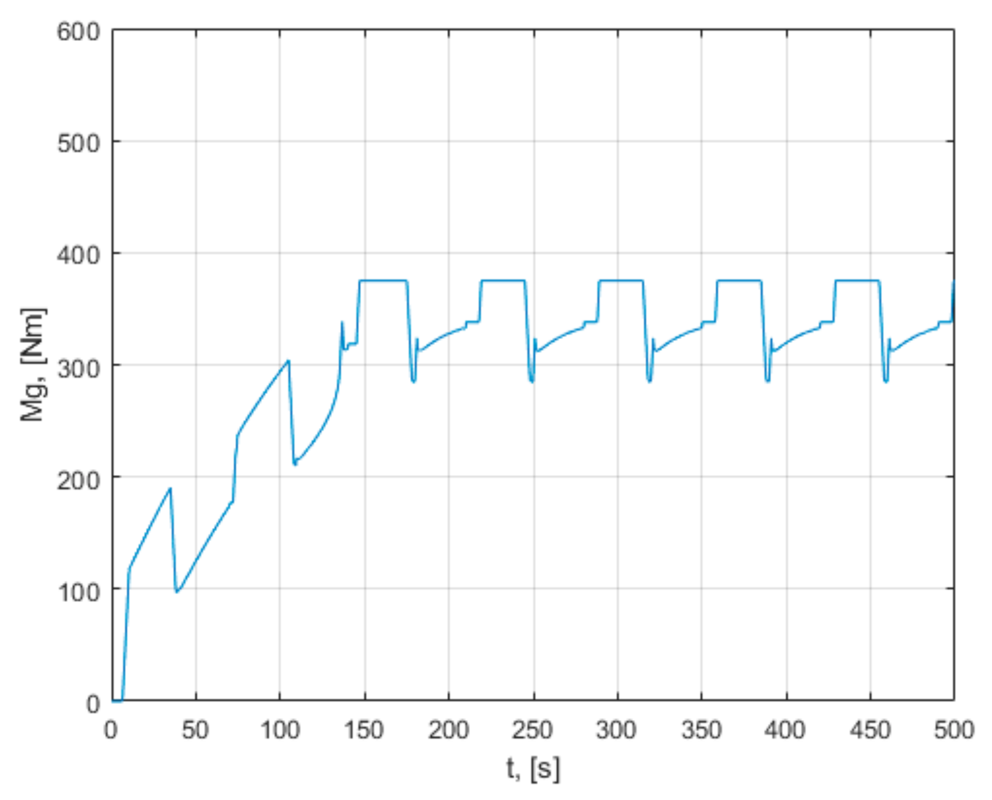
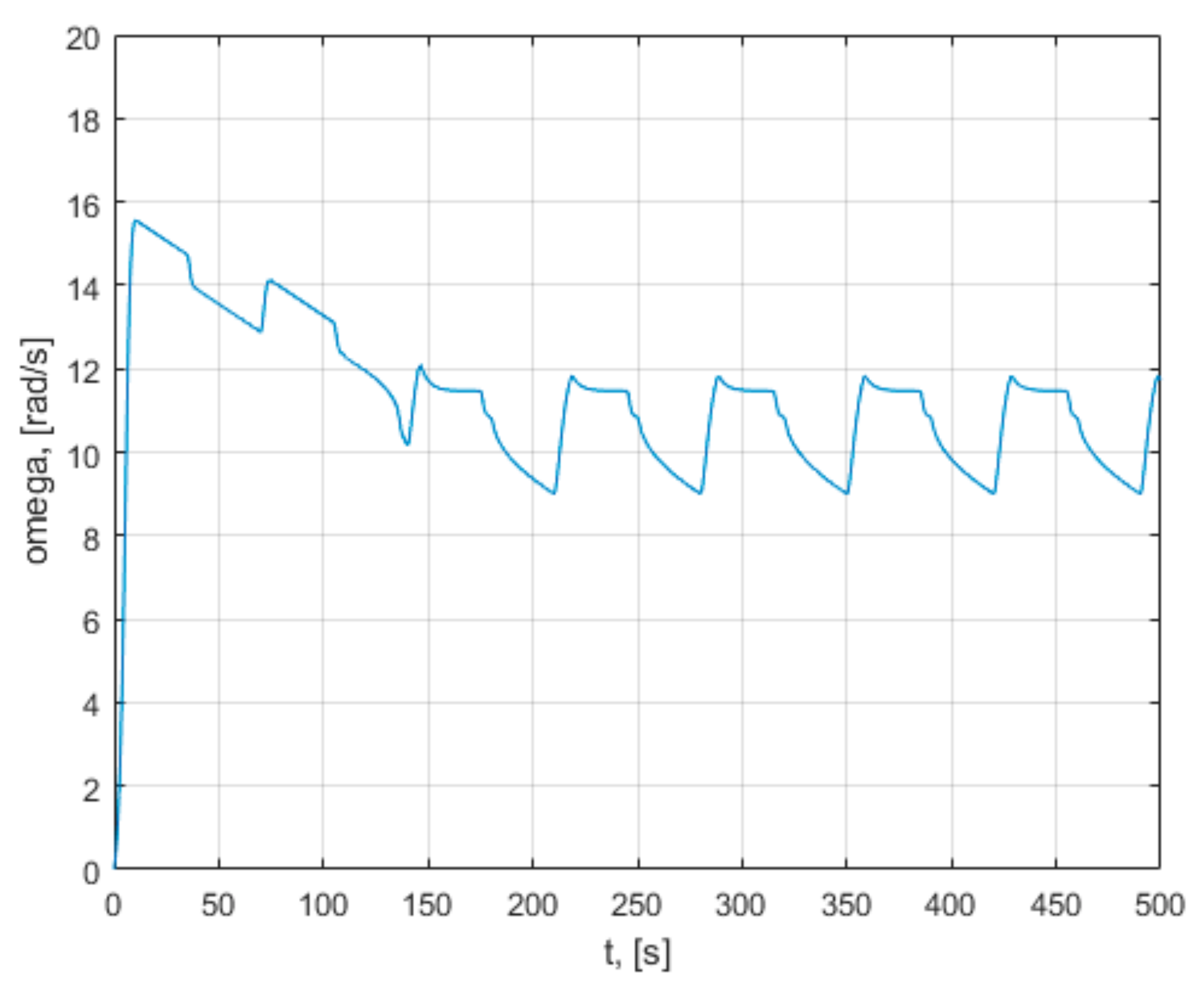
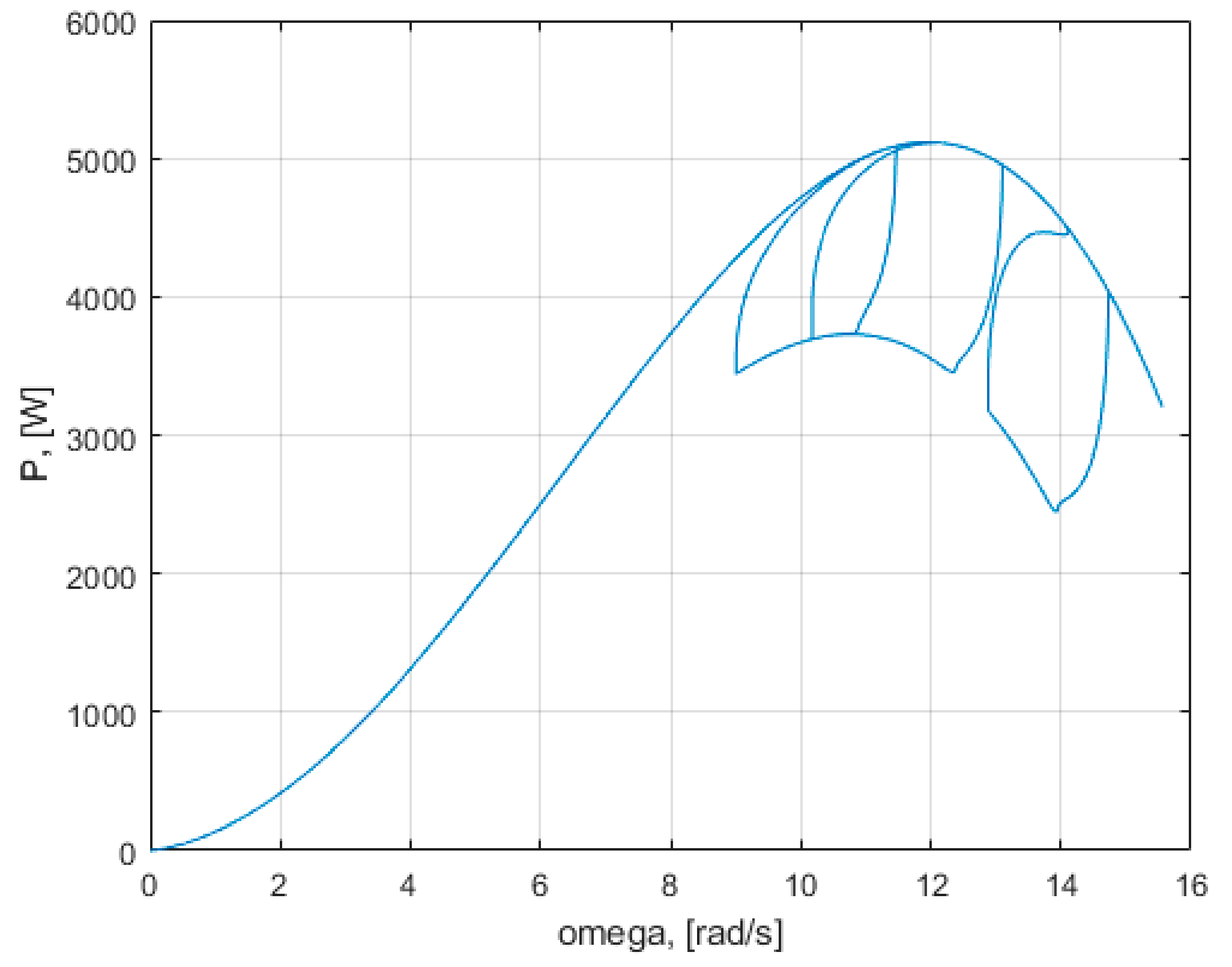
The characteristics obtained in a dynamic regime for an unfavorable operation case, in which a constant, low value of the load torque is considered, are presented in Appendix A. Those characteristics demonstrate that the turbine model behaves according to the presented relations. It is observed that the turbine variable values change with the change in wind speed and load torque. From the presented graphs, it is observed that the operating point of the turbine passes from one characteristic of the speed to another, together with the change in the wind speed and the change in the load torque. This simulation demonstrates that changing the load torque can change the rotational speed, the power generated, and the operating point. If the load torque increases, the operating point tends to move to the maximum power points. The peaks that appear on the characteristics of the variables are due to the sudden changes in the velocity v, which intervene in the calculations at the denominator of the relation of λ. In the condition in which the turbine operates at a low constant load torque, without being driven with maximum power point tracking, the installation reaches a steady state, with operating points far from the maximum power point. This makes it necessary to use methods of maximum power point tracking. The maximum co-ordinate power points (ω, P_max,) in the phase plane are unstable equilibrium points. The turbine has an infinite number of unstable equilibrium points. The main disadvantage of turbine control systems is due to this fact, namely, that it is desired that the operating points of the system be precisely these points of unstable equilibrium. The tendency of the system in the equilibrium point is important. The system does not return to the equilibrium point if a small initial condition offset is used or it is moved away from the equilibrium point.

A set of nine maximum power point tracking rules has been developed and implemented in the control methods. The control rules for tracking the maximum power point were developed based on a human reasoning, taking into account the physical phenomenon that occurs in the installation: the dynamics of the rotational movement of the turbine shaft and electromagnetic phenomena that occur in the electric generator.

The maximum power point tracking rules have been adapted for on–off control and for fuzzy control in a numerical manner.

The developed maximum power point tracking rules lead the turbine on various state trajectories closer to the maximum power point. The maximum power point tracking rules suit on–off driving with dead band, which has only three states.

The variables at the controller inputs have continuous values over time. The variable at the output of the regulator is in the form of a three-state pulse train. In the case of on–off control, in the first phase, in a transient state, the trajectories are further away from the optimal trajectory. The transient state lasts longer than in the case of the other two methods. It is observed that, in steady state, the operating point approaches the maximum. The operating point moves between the characteristics of 9 and 10 m/s.

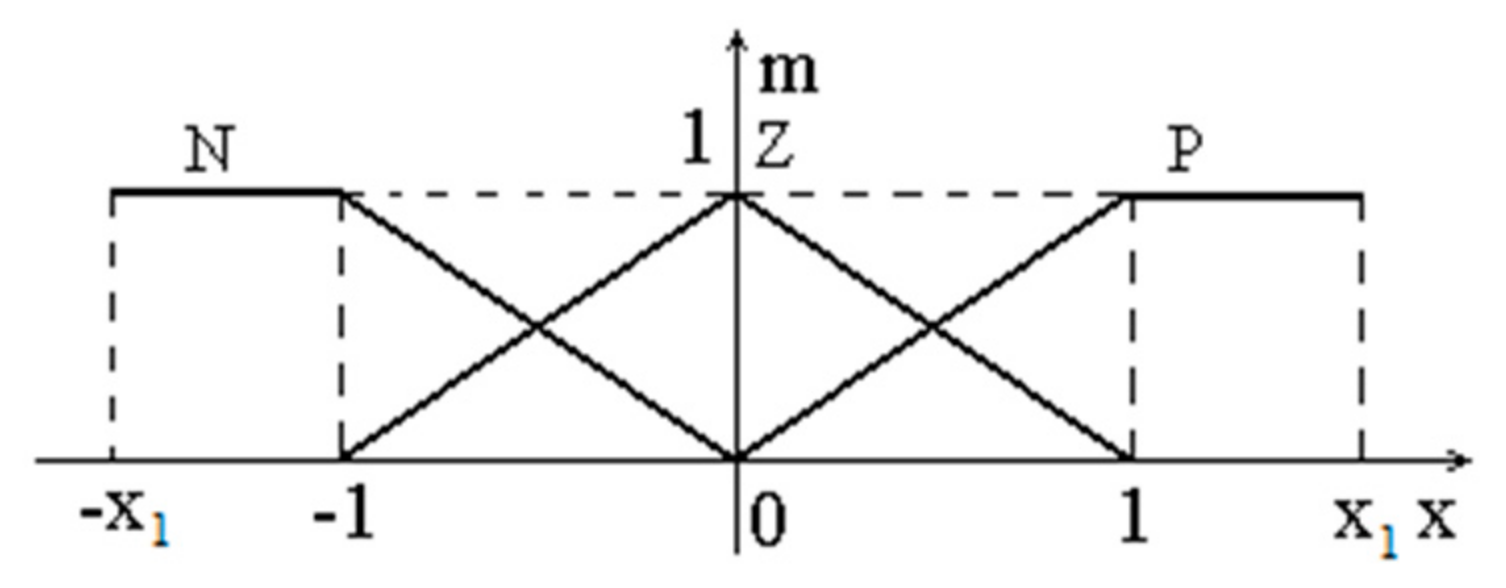
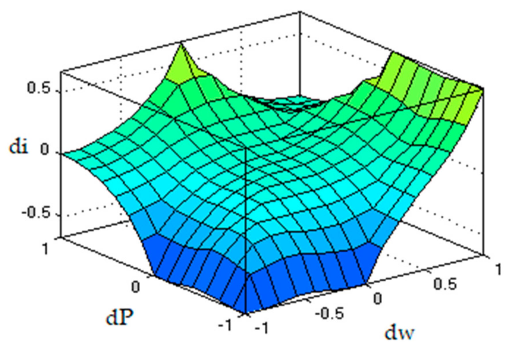
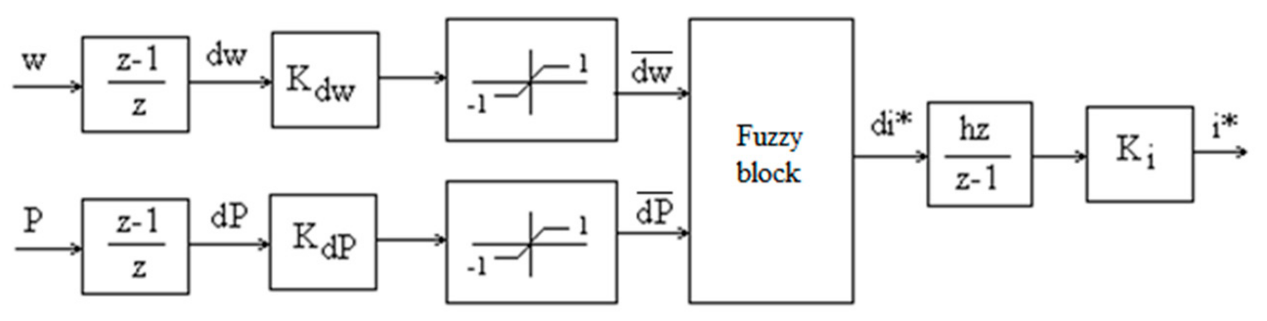
In this case, the behavior of the control system depends on the choice of the amplification coefficient of current reference. A block with Mamdani’s structure was used in the fuzzy controller. A base with nine rules was used, identical to the rules of the tracking method. Three fuzzy variables were used for each variable of the regulator, with three membership functions, triangular and trapezoidal. This structure gives the most nonlinear character of the fuzzy controller.

Unlike on–off control, fuzzy logic ensures interpolation between rules. In addition, in the case of fuzzy control, the state trajectories are closer to the ideal trajectory of the search for the maximum power point.

In the case of fuzzy regulation, a shorter transient regime was obtained following repeated simulation tests.

The operating point moves from the 10 m/s characteristic to the 9 m/s characteristic on the state trajectories close to the maximum power trajectory. The control system reaches the same points after the change in wind speed, close to the maximum point.

In this case, the choice of amplification coefficients of the fuzzy controller must be made carefully.

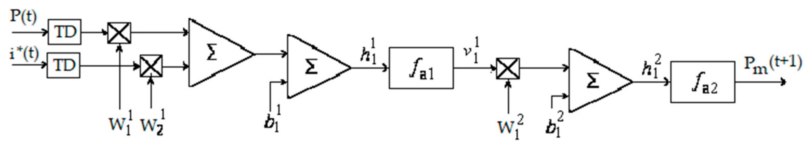
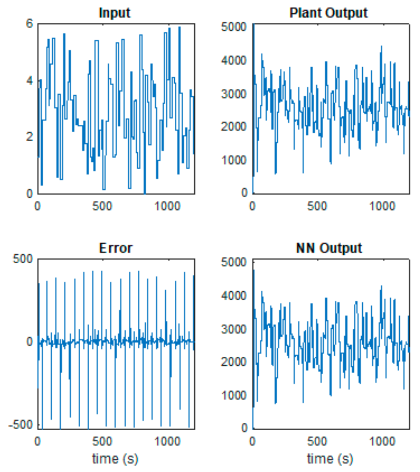
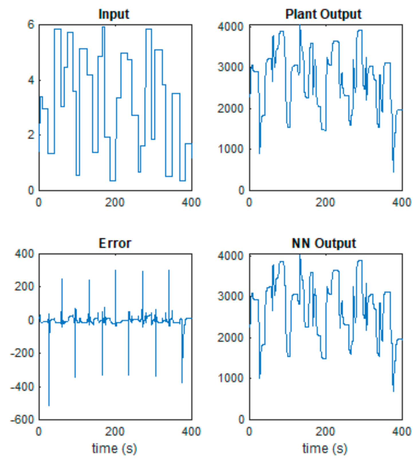
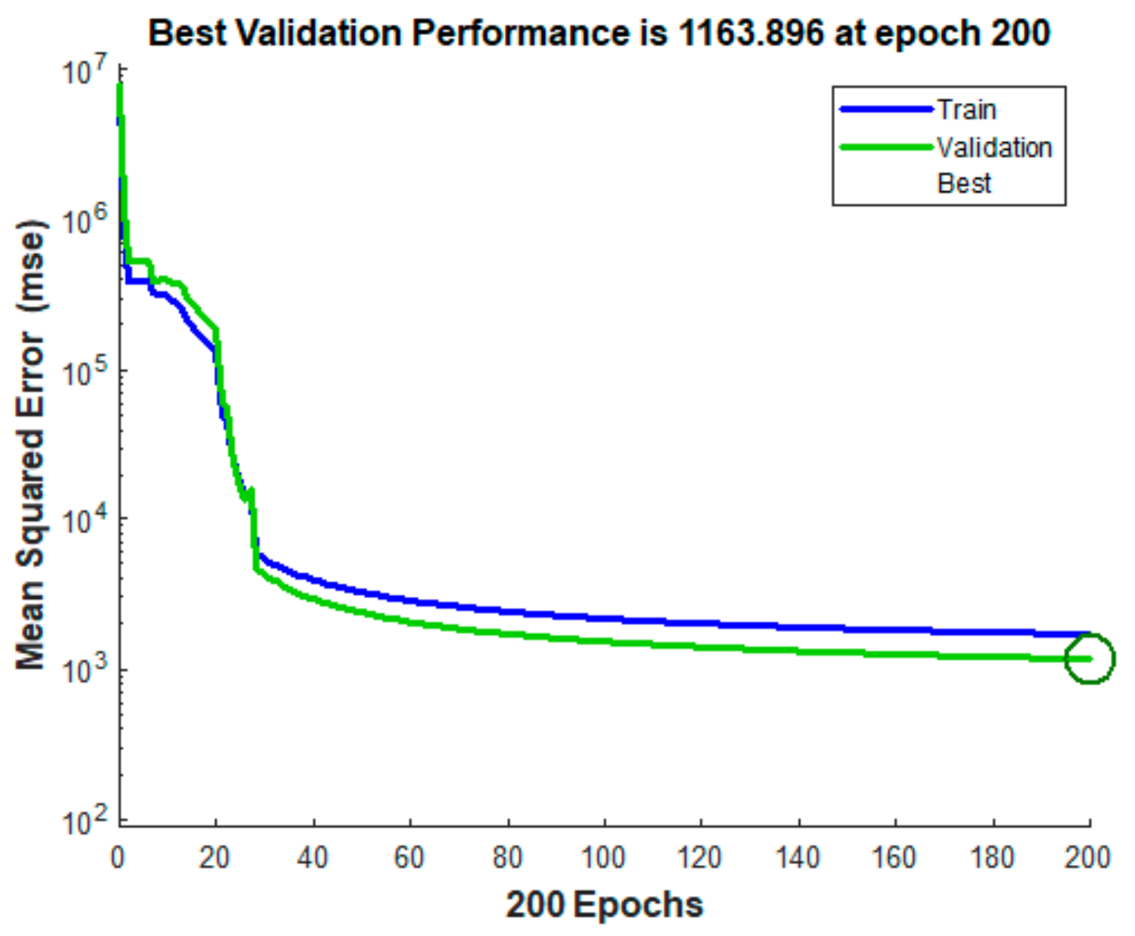
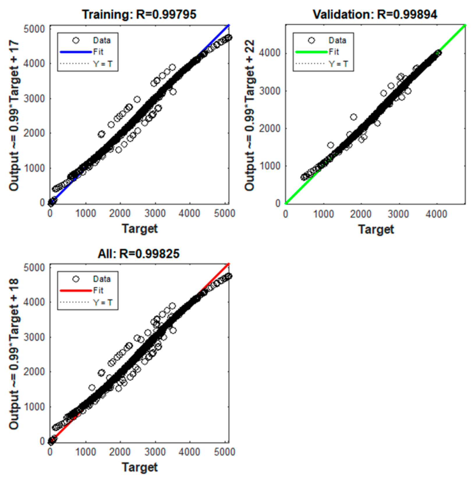
A fuzzy block with Sugeno’s structure, and other forms of membership functions, may also be tested as a future direction of research. It is recommended to test fuzzy controllers with more rules, more fuzzy variables, and more membership functions. For example, with five fuzzy values, such as: negative big, negative small, zero, positive small, positive big. This regulator could more precisely capture particular parts of the maximum power point tracking. However, it will lose the nonlinearity of the regulation, which is the main characteristic of the fuzzy controller. The use of deep learning techniques allows the identification of the wind turbine with a neural network model and the introduction of a neural predictive control method. The identification can be done offline using data taken from the wind turbine. The process of training the neural networks used as a model and as a regulator is a complex process, requiring several phases and a long computation time. This process requires significant computing resources, both a high computational speed and a high computational memory. The amplitudes of the uniformly distributed random signal must be chosen in the maximum value range of the system variables. The Levenberg–Marquardt neural training method ensures a small mean squared error is obtained after a shorter training time than in the case of other methods. It does not get stuck in local minima. In the presented example, a structure with the lowest value of mean squared error was chosen. From the simulations, it results that the presented solution has a longer duration of the transient state than in the case of fuzzy regulation. It is observed that the generated power follows the prescribed power with a certain error, and the state trajectories are around the optimal trajectory. A better identification of the process and a better dimensioning of the prediction law could be tried. Other neural network structures with different numbers of layers and neurons can be tested as a future direction of research. Different trainings lead to different structures of the neural network and to different values of weights and biases.

Analyzing the characteristics (ω, P), it is observed that, in the first part of the transient state, all the control methods bring the operating point on the same characteristic for the same wind speed.

One of the main findings is that the energy generated increases significantly in cases that follow the maximum power point, up to 60%, compared to the case of operating at a low and constant load torque and without maximum power point tracking, as can be seen in Table 4.

A second finding is that the differences between the energies generated at the various analyzed methods of maximum power point tracking are small, as can be seen in Table 4. The maximum difference is 5%, compared to the fuzzy control. In addition, between neural control and on–off control, the difference is not more than 0.7%. If there are discrepancies in the amplification coefficients in practice, the characteristics may deteriorate. It must also be taken into account that efficiency of the electric generator is higher at the rated speed and decreases when the speed decreases.

Because the implementation of control techniques is numerical, the choice of the sampling period and the methods of numerical approximation of derivation and integration must be made appropriately with the dynamics of the process. The transient state is longer, as in the case of on–off control, due to the method, but also due to the amplification coefficients of the regulator and the sampling mode.

6. Conclusions

The paper analyzed three mathematical methods for maximum power point tracking, namely, on–off control, fuzzy control, and neural predictive control. The results obtained with the three control methods were compared based on the energy generated, chosen as a performance indicator. Working at variable speeds using the method of tracking, the maximum power point increases the energy generated. The increase is maximum compared to the worst case of operation, with low and constant load torque. However, if the load torque approaches the maximum power point, in the case of no regulation, the energy generated in this case increases, and the energy generated in the case of maximum power point tracking could not be significantly higher. The use of various control methods to track the maximum power point did not lead to major differences in the energy generated. However, the differences from the energetic point of view between the analyzed control methods are small. The analyzed methods fail to eliminate the main disadvantage that the maximum power point is an unstable equilibrium point. Finding a way to stabilize the control system in the maximum power point could be a direction of research. Most of the time, during the entire control process, these methods lead the system on various trajectories in suboptimal states. Moreover, the big challenge of choosing the coefficients of the regulators remains. Future directions of research may be to try other set of rules, finding more detailed rules of maximum power point tracking that capture behaviors in narrow domains, and to make new comparative studies.