Robust Stabilization and Observer-Based Stabilization for a Class of Singularly Perturbed Bilinear Systems

Abstract

An infinite-bound stabilization of a system modeled as singularly perturbed bilinear systems is examined. First, we present a Lyapunov equation approach for the stabilization of singularly perturbed bilinear systems for all ε∈(0, ∞). The method is based on the Lyapunov stability theorem. The state feedback constant gain can be determined from the admissible region of the convex polygon. Secondly, we extend this technique to study the observer and observer-based controller of singularly perturbed bilinear systems for all ε∈(0, ∞). Concerning this problem, there are two different methods to design the observer and observer-based controller: one is that the estimator gain can be calculated with known bounded input, the other is that the input gain can be calculated with known observer gain. The main advantage of this approach is that we can preserve the characteristic of the composite controller, i.e., the whole dimensional process can be separated into two subsystems. Moreover, the presented stabilization design ensures the stability for all ε∈(0, ∞). A numeral example is given to compare the new ε-bound with that of previous literature.

1. Introduction

As is well known, a large class of physical systems in biology, engineering, ecology, socio-economics, nuclear, thermal, and chemical processes can be properly described by bilinear models [1,2,3,4]. The above-mentioned systems are usually described by higher-order dimensional types. Due to the high-order dimensions of these factories, a large amount of computer memory and considerable operating time are required to process such a large-scale system. The singular perturbation method [5,6,7,8,9,10,11,12,13,14,15,16] is very useful for solving the problems of high dimensionality and stiffness when dealing with large-scale systems. Although the singularly perturbed systems have so many applications and combinations with other methodologies, apparently many basic issues remain to further address. Especially, stability analysis and controller design are fundamental issues for singularly perturbed systems. It is well known that stabilizing the slow and fast subsystems will not guarantee the stability of the resulting closed-loop system for all singular parameters. Therefore, it is of great importance to find the singular parameter bound for the stability of reduced and closed-loop systems. Many papers have tried various ways to calculate the bound, but only sufficiently small bound for ε are available and some of them are rather conservative. The controller design of this type of model is costly to implement, and sometimes even impossible to implement.

However, thus far, there are few literatures on the stabilization of singularly perturbed bilinear systems [17,18,19,20]. Literature [17] uses Lyapunov’s theory to study the stabilization of singularly perturbed strictly bilinear systems. Asamoah and Jamshidi [18] extended the results of [19] to singularly perturbed bilinear systems, but some of the results in [17] were proven wrong by [19]. These papers [17,18,19] only guarantee the stability for ε∈(0, 1). The above results [17,18,19] seem to be limited to continuous time. For discrete system, Ref. [20] presented two kinds of robust controllers for stabilizing singularly perturbed discrete bilinear systems. That is, all stable solutions can be implemented under the assumption that all states are available for measurement. This assumption is usually not true in practice, that is, the state of the system may not be able to achieve state feedback. Therefore, it is usually necessary to design an observer and a controller, which leads to the asymptotic stability of a given equilibrium point [21].

In this paper, an infinite ε-bound stabilization of a system modeled as singularly perturbed bilinear systems is examined. First, we present a Lyapunov equation for the stabilization of singularly perturbed bilinear systems for all ε∈(0, ∞). The method is based on the Lyapunov stability theorem. The state feedback constant gain can be determined from the admissible region of the convex polygon. Second, we extend this technique to study the observer and observer-based controller of singularly perturbed bilinear systems for all ε∈(0, ∞). Where two different methods are proposed to design the observer and observer-based control gains, one is the estimator’s gain can be calculated with known bounded input, and the other is the state feedback gain can be calculated with known observer’s gain. The main advantage of the developed schemes is that the whole dimensional design can be directly separated into two lower dimensions without the decomposition and composition of the slow and fast subsystems. Moreover, the presented design insures the stability for all ε∈(0, ∞). We show by example that the new ε-bound can yield the maximum robust stability bound than that of the result [18].

The following notations will be used throughout the paper: the identity matrix with dimension n is denoted by In, λ(A) stands for the eigenvalues of matrix A, $\parallel A\parallel$ denotes the norm of matrix A, i.e., $\parallel A\parallel =Max{[\lambda \left(A^{T}A\right)]}^{1/2}$.

2. Problem Formulation and Design Procedure

Consider the linear time-invariant singularly perturbed bilinear system

$$\left[\begin{array}{c}{\dot{x}}_1\left(t\right)\\ \epsilon {\dot{x}}_2\left(t\right)\end{array}\right]=\left[\begin{array}{cc}{A}_{11}& A_{12}\\ A_{21}& A_{22}\end{array}\right]\left[\begin{array}{c}{x}_1\left(t\right)\\ x_2\left(t\right)\end{array}\right]+\left[\begin{array}{cc}{N}_{11}& N_{12}\\ N_{21}& N_{22}\end{array}\right]\left[\begin{array}{c}{x}_1\left(t\right)\\ x_2\left(t\right)\end{array}\right]u\left(t\right)+\left[\begin{array}{c}{B}_1\\ B_2\end{array}\right]u\left(t\right)$$

$$y\left(t\right)=C_1{x}_1\left(t\right)+C_2{x}_2\left(t\right)$$

(1)

where $x_1\in R^{n_1}$, $x_2\in R^{n_2}$, n(= n₁ + n₂) is the order of the whole system, u ∈R is the control, $y\in R^m$ is the output and the matrices $A_{ij}$, $N_{ij}$, $B_i$ and $C_i$ are constant matrices with appropriate dimensions for i, j = 1, 2, and ε is the singular perturbation parameter.

2.1. Nonlinear State Feedback

First, the main objective of this subsection is to design a nonlinear state feedback controller for the given system (1) to be stable with ε∈(0, ∞). Here, we will apply a control of the form

$$u\left(t\right)=-\frac{k_1{D}_1{x}_1}{\sqrt{1+x_1^T{D}_1^T{D}_1{x}_1}}-\frac{k_2{D}_2{x}_2}{\sqrt{1+x_2^T{D}_2^T{D}_2{x}_2}}$$

(2)

to stabilize the system (1), where $D_i\in R^{1\times n_i}$ can be arbitrarily designed, and $K_i$ are constants. To investigate the stability of system (1), we choose the Lyapunov function candidate as

$$V\left(x_1, x_2\right)=x_1^T{P}_1{x}_1+\epsilon x_2^T{P}_2{x}_2$$

(3)

where $P_i\in R^{n_i\times n_i}$ are unique real symmetric positive-definite matrices satisfying the Lyapunov equations,

$$A_{ii}^T{P}_i+P_i{A}_{ii}=-2I_{n_i}$$

(4)

for i = 1, 2, and $A_{ii}$ are assumed to be stable.

Remark 1.

The system’s input can be deterministic signals with unknown upper bounds, i.e.,$u\left(t\right)\in \Omega$and$\Omega \triangleq \left\{u\left(t\right)|\left|u\left(t\right)\right|\le \left|k_1\right|+\left|k_2\right|\right\}$.

Substitution of (2) into (1) yields an alternative form

$$\left[\begin{array}{c}{\dot{x}}_1\\ {\dot{x}}_2\end{array}\right]=\left[\begin{array}{cc}{\overline{A}}_{11}& {\overline{A}}_{12}\\ {\overline{A}}_{21}& {\overline{A}}_{22}\end{array}\right]\left[\begin{array}{c}{x}_1\left(t\right)\\ x_2\left(t\right)\end{array}\right]$$

(5)

where

$${\overline{A}}_{ii}=A_{ii}-k_i{N}_{ii}\sin {\theta }_i-k_j{N}_{ii}\sin {\theta }_j-k_i{B}_i{D}_i\cos {\theta }_i$$

$${\overline{A}}_{ij}=A_{ij}-k_i{N}_{ij}\sin {\theta }_i-k_j{N}_{ij}\sin {\theta }_j-k_j{B}_i{D}_j\cos {\theta }_j$$

$$\sin {\theta }_i=\frac{x_i^T{D}_i^T}{\sqrt{1+x_i^T{D}_i^T{D}_i{x}_i}},·\cos {\theta }_i=\frac{1}{\sqrt{1+x_i^T{D}_i^T{D}_i{x}_i}} \mathrm{and} -{90}^{°}\le {\theta }_i\le {90}^{°} \mathrm{for} i=1, 2.$$

Before deriving the main result, one preliminary lemma is reviewed firstly.

Lemma 1 ([22]).

For any matrices X and Y with appropriate dimensions, we have

$$X^{T}Y+Y^{T}X\le \gamma X^{T}X+Y^{T}Y$$

(6)

for any constant γ >0.

Theorem 1.

Consider the singularly perturbed bilinear system (1) and assume that Aii is Hurwitz and$\parallel P_i{A}_{ij}{A}_{ij}^T{P}_i\parallel <1$, if$k_1$and$k_2$are selected inside the region of the convex polygon as shown in Figure 1, the nonlinear state feedback controller (2) stabilizes the system (1) in the entire state space for all ε∈(0, ∞), where the four intersections of convex polygon with$k_1$–axis and with$k_2$–axis are described follows,

$${\overline{k}}_1=\left(1-\parallel P_1{A}_{12}{A}_{12}^T{P}_1\parallel \right)/\left(2\parallel N_{11}^T{P}_1\parallel +2\parallel D_1^T{B}_1^T{P}_1\parallel +\parallel P_1{N}_{12}{N}_{12}^T{P}_1\parallel +2\right)$$

$${\widehat{k}}_1=\left(1-\parallel P_2{A}_{21}{A}_{21}^T{P}_2\parallel \right)/\left(2\parallel N_{22}^T{P}_2\parallel +\parallel P_2{N}_{21}{N}_{21}^T{P}_2\parallel +\parallel P_2{B}_2{D}_1{D}_1^T{B}_2^T{P}_2\parallel +1\right)$$

$${\overline{k}}_2=\left(1-\parallel P_1{A}_{12}{A}_{12}^T{P}_1\parallel \right)/\left(2\parallel N_{11}^T{P}_1\parallel +\parallel P_1{N}_{12}{N}_{12}^T{P}_1\parallel +\parallel P_1{B}_1{D}_2{D}_2^T{B}_1^T{P}_1\parallel +1\right)$$

$${\widehat{k}}_2=\left(1-\parallel P_2{A}_{21}{A}_{21}^T{P}_2\parallel \right)/\left(2\parallel N_{22}^T{P}_2\parallel +2\parallel D_2^T{B}_2^T{P}_2\parallel +\parallel P_2{N}_{21}{N}_{21}^T{P}_2\parallel +2\right)$$

(7)

Proof. 

From (3), (5) and Lemma 1, the Lyapunov function’s derivative becomes

$$\begin{gathered} \dot{V}={\dot{x}}_1^T{P}_1{x}_1+x_1^T{P}_1{\dot{x}}_1+\epsilon {\dot{x}}_2^T{P}_2{x}_2+\epsilon x_2^T{P}_2{\dot{x}}_2 \\ ={\displaystyle \sum }_{i=1}^2[{({\overline{A}}_{ii}{x}_i+{\overline{A}}_{ij}{x}_j)}^T{P}_i{x}_i+x_i^T{P}_i\left({\overline{A}}_{ii}{x}_i+{\overline{A}}_{ij}{x}_j\right)] (\mathrm{for} j=1,2, \mathrm{and} j\ne i) \\ ={\displaystyle \sum }_{i=1}^2[2x_i^T\left(A_{ii}^T{P}_i-k_i{N}_{ii}^T{P}_i\sin {\theta }_i-k_j{N}_{ii}^T{P}_i\sin {\theta }_j-k_i{D}_i^T{B}_i^T{P}_i\cos {\theta }_i\right)x_i \\ +2x_j^T\left(A_{ij}^T{P}_i-k_i{N}_{ij}^T{P}_i\sin {\theta }_i-k_j{N}_{ij}^T\sin {\theta }_j-k_j{D}_j^T{B}_i^T{P}_i\cos {\theta }_j\right)x_i] \\ \le {\displaystyle \sum }_{i=1}^2{x}_i^T[-1+\parallel P_i{A}_{ij}{A}_{ij}^T{P}_i\parallel +\left|k_i\right|\left(2\parallel N_{ii}^T{P}_i\parallel +2\parallel C_i^T{B}_i^T{P}_i\parallel +\parallel P_i{N}_{ij}{N}_{ij}^T{P}_i\parallel +2\right) \\ +\left|k_j\right|\left(2\parallel N_{ii}^T{P}_i\parallel +\parallel P_i{B}_i{D}_j{D}_j^T{B}_i^T{P}_i\parallel +\parallel P_i{N}_{ij}{N}_{ij}^T{P}_i\parallel +1\right)]x_i \end{gathered}$$

It is easily verified that the following inequality holds such that $\dot{V}<0$

$$\begin{gathered} -1+\parallel P_i{A}_{ij}{A}_{ij}^T{P}_i\parallel +\left|k_i\right|\left(2\parallel N_{ii}^T{P}_i\parallel +2\parallel D_i^T{B}_i^T{P}_i\parallel +\parallel P_i{N}_{ij}{N}_{ij}^T{P}_i\parallel +2\right) \\ +\left|k_j\right|\left(2\parallel N_{ii}^T{P}_i\parallel +\parallel P_i{B}_i{D}_j{D}_j^T{B}_i^T{P}_i\parallel +\parallel P_i{N}_{ij}{N}_{ij}^T{P}_i\parallel +1\right)<0 \end{gathered}$$

(8)

From the above inequality (8), the eight pinnacles on the coordinate axes of $k_1-k_2$ plane form a convex polygon as shown in Figure 1. Hence, the controller (2), whose gains are selected inside the admissible region of Figure 1, can stabilize the system (1) for all ε∈(0, ∞). □

Remark 2.

Singular perturbation technique is usually a method to deal with two-time-scale systems, where the analysis of the whole system can be split, for “small” values of ε (or the limit$\epsilon \to 0$), into the analysis of two separate systems presented in the slow and fast time scales. One tries to design a controller for the whole system working on reduced order control problems for the two limit systems. In this paper, we do not utilize the time-scale properties of the system and this is another reason why asymptotic stability is guaranteed also for “large” ε, though the two-time-scale structure of the system may be destroyed. In fact, no information is given to determine whether or not the two-time-scale separation is preserved in the closed-loop case as ε approaches the maximum upper bound ε*. Note that we seek the maximum upper bound ε* for the closed-loop system to retain stable, the value of ε* with which we end up might turn out to be not so small (sometimes even infinite) [23]. As such, the calculation of ε* serves only one purpose, namely it guarantees that the system (1) is well behaved in the generalized stability sense for all ε∈(0, ε*).

Remark 3.

The hypotheses employed by Theorem 1, i.e., asymptotic stability of matrices$A_{11} and A_{22}$, and inequalities$\parallel P_1{A}_{12}{A}_{12}^T{P}_1\parallel <1, \parallel P_2{A}_{21}{A}_{21}^T{P}_2\parallel <1$, guarantee that the open-loop system is asymptotically stable for any value of ε∈(0,∞). One can notice that the polygon of admissible gains given in Theorem 1 includes the origin of the$k_1-k_2$plane. One query may raise. What is the reason to apply a closed-loop control to stabilize a stable system (1)? There is at least a main reason to show the necessity of the feedback control: It is well known that an open-loop system is sensitive for some parameter variations or external input disturbances. In other words, if u(t) = 0, the bilinear system becomes an open-loop linear system, which may be unstable easily under some external disturbances. But by the given nonlinear feedback control (2), the robust stability of the system will increase [2].

Remark 4.

There have been some papers as well [24,25,26] discussing the stabilization problem of the bilinear system with the open-loop stable system.

2.2. Observer and Observer-Based State Feedback

Furthermore, the objective of the subsection is to design a full state observer and observer-based feedback for the given system (1) to be stable with ε∈(0, ∞). Now, it is required to construct an observer dynamical equation for the system (1) as below:

$${\dot{\widehat{x}}}_1=A_{11}{\widehat{x}}_1+A_{12}{\widehat{x}}_2+N_{11}{\widehat{x}}_{1}u+N_{12}{\widehat{x}}_{2}u+B_{1}u+L_1\left(y-C_1{\widehat{x}}_1-C_2{\widehat{x}}_2\right)$$

$$\epsilon {\dot{\widehat{x}}}_2=A_{21}{\widehat{x}}_1+A_{22}{\widehat{x}}_2+N_{21}{\widehat{x}}_{1}u+N_{22}{\widehat{x}}_{2}u+B_{2}u+L_2\left(y-C_1{\widehat{x}}_1-C_2{\widehat{x}}_2\right)$$

(9)

where ${\widehat{x}}_1\in R^{n_1}, {\widehat{x}}_2\in R^{n_2}$ are the observer states, and $L_1\in R^{n_1\times q}$ and $L_2\in R^{n_2\times q}$ are suitable observing gain matrices that will be designed so as to ensure the estimated state ${\widehat{x}}_1\to x_1 \mathrm{and} {\widehat{x}}_2\to x_2$ as $t\to \infty$. It should also be added that the pair $\left(A_i,C_i\right)$ is detectable.

Here, we will apply an observer-based feedback of the form

$$\begin{gathered} u\left(t\right)=-\frac{k_1{D}_1{\widehat{x}}_1}{\sqrt{1+{\widehat{x}}_1^T{D}_1^T{C}_1{\widehat{x}}_1}}-\frac{k_2{D}_2{\widehat{x}}_2}{\sqrt{1+{\widehat{x}}_2^T{D}_2^T{D}_2{\widehat{x}}_2}} \\ =-k_1\sin {\widehat{\theta }}_1-k_2\sin {\widehat{\theta }}_2 \\ =-k_1\cos {\widehat{\theta }}_1{D}_1{\widehat{x}}_1-k_2\cos {\widehat{\theta }}_2{D}_2{\widehat{x}}_2 \end{gathered}$$

(10)

to stabilize the system (1), where $D_i\in R^{1\times n_i}$ can be arbitrarily designed, $k_i$ is constants, $\sin {\widehat{\theta }}_i=\frac{{\widehat{x}}_i^T{D}_i^T}{\sqrt{1+{\widehat{x}}_i^T{D}_i^T{D}_i{\widehat{x}}_i}},$ $\cos {\widehat{\theta }}_i=\frac{1}{\sqrt{1+{\widehat{x}}_i^T{D}_i^T{D}_i{\widehat{x}}_i}}$ and $-{90}^{°}\le {\widehat{\theta }}_i\le {90}^{°}$ for i = 1, 2.

Hence, we obtain the state and error $\left(e_1=x_1-{\widehat{x}}_1 \mathrm{and} e_2=x_2-{\widehat{x}}_2\right)$ equations which can be written as follows,

$$\left[\begin{array}{c}{\dot{x}}_1\\ \epsilon {\dot{x}}_2\end{array}\right]={\widehat{A}}_{11}\left[\begin{array}{c}{x}_1\\ x_2\end{array}\right]+{\widehat{A}}_{12}\left[\begin{array}{c}{e}_1\\ e_2\end{array}\right]$$

$$\left[\begin{array}{c}{\dot{e}}_1\\ \epsilon {\dot{e}}_2\end{array}\right]={\widehat{A}}_{21}\left[\begin{array}{c}{x}_1\\ x_2\end{array}\right]+{\widehat{A}}_{22}\left[\begin{array}{c}{e}_1\\ e_2\end{array}\right]$$

(11)

where

$${\widehat{A}}_{11}=\left[\begin{array}{cc}{\overline{A}}_{11}& {\overline{A}}_{12}\\ {\overline{A}}_{21}& {\overline{A}}_{11}\end{array}\right], {\widehat{A}}_{12}=\left[\begin{array}{cc}{k}_1{B}_1{D}_1\cos {\widehat{\theta }}_1& k_2{B}_1{D}_2\cos {\widehat{\theta }}_2\\ k_1{B}_2{D}_1\cos {\widehat{\theta }}_1& k_2{B}_2{D}_2\cos {\widehat{\theta }}_2\end{array}\right], {\widehat{A}}_{21}=0 \mathrm{and} {\widehat{A}}_{22}=\left[\begin{array}{cc}{\tilde{A}}_{11}& {\tilde{A}}_{12}\\ {\tilde{A}}_{21}& {\tilde{A}}_{22}\end{array}\right],$$

in which ${\tilde{A}}_{ii}={\overline{A}}_{ii}-k_i{N}_{ii}\sin {\widehat{\theta }}_i-k_j{N}_{ii}\sin {\widehat{\theta }}_j$, ${\tilde{A}}_{ij}={\overline{A}}_{ij}-k_i{N}_{ij}\sin {\widehat{\theta }}_i-k_j{N}_{ij}\sin {\widehat{\theta }}_j$, and ${\overline{A}}_{ii}=A_{ii}-L_i{C}_i, {\overline{A}}_{ij}=A_{ij}-L_i{C}_j$ for $i,j=1,2,i\ne j.$

For the stability of the system (11), the eigenvalues of ${\widehat{A}}_{11} \mathrm{and} {\widehat{A}}_{22}$ are designed within the unit circle, i.e., $|\lambda ({\widehat{A}}_{11})|<1$ and $|\lambda ({\widehat{A}}_{22})|<1$. The objective is to find the suitable estimator matrices $L_1$ and $L_2$ such that the estimated error approaches zero. This means that the estimated state ${\widehat{x}}_1$ and ${\widehat{x}}_2$ can approach the real state $x_1$ and $x_2$ for all ε∈(0, ∞), respectively.

In order to prove the stability of the error Equation (11), the Lyapunov function candidate is given by

$$V\left(e_1,e_2\right)=e_1^T{P}_{o1}{e}_1+\epsilon e_2^T{P}_{o2}{e}_2$$

(12)

where $P_{oi}\in R^{n_i\times n_i}$ are unique real symmetric positive-definite matrices satisfying the Lyapunov equations,

$${\overline{A}}_{ii}^T{P}_{oi}+P_{oi}{\overline{A}}_{ii}=-2I_{n_i}$$

(13)

for i = 1, 2, and ${\overline{A}}_{ii}$ are assumed to be stable.

Theorem 2.

For the singularly perturbed bilinear systems (1) with observer-based controller (10), in which$k_1$and$k_2$can be calculated from Theorem 1. If there exist$L_1$and$L_2$such that

$$\parallel P_{oi}{\overline{A}}_{ij}{\overline{A}}_{ij}^T{P}_{oi}\parallel <1-(2\parallel N_{ii}^T{P}_{oi}\parallel +\parallel P_{oi}{N}_{ij}{N}_{ij}^T{P}_{oi}\parallel +1)\left(\left|k_1\right|+\left|k_2\right|\right)$$

(14)

Then the system (11) is asymptotically stable for all ε∈(0, ∞).

Proof. 

The proof can be divided into two parts:

(i)

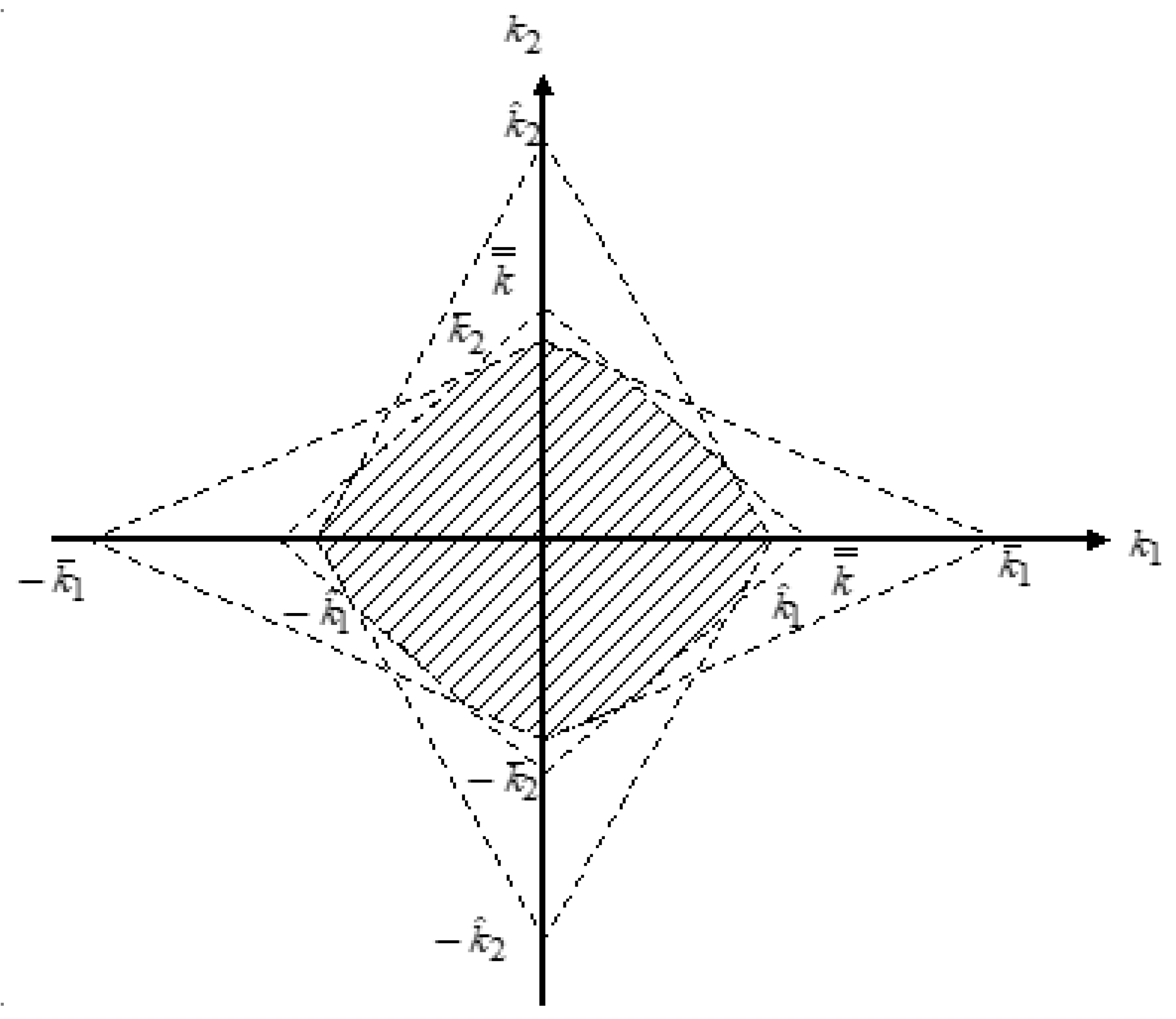
The stability of the system’s state Equation (11).

In fact, this result is the same as Theorem 1, i.e., if $x_1\in R^{n_1}$ are selected inside the region of the convex polygon as shown in Figure 1, then ${\widehat{A}}_{11}$ can be guaranteed to be stable.

(ii)

The stability of the error Equation (11).

From (11), (12) and Lemma 1, the Lyapunov function’s derivative becomes

$$\begin{gathered} \dot{V}\left(e_1,e_2\right)={\dot{e}}_1^T{P}_{oi}{e}_1+e_1^T{P}_{oi}{\dot{e}}_1+\epsilon {\dot{e}}_2^T{P}_{oi}{e}_2+\epsilon e_2^T{P}_{oi}{\dot{e}}_2 \\ ={\displaystyle \sum }_{i=1}^2[({\tilde{A}}_{ii}{e}_i+{\tilde{A}}_{ij}{e}_j{)}^T{P}_{oi}{e}_i+e_i^T{P}_{oi}({\tilde{A}}_{ii}{e}_i+{\tilde{A}}_{ij}{e}_j)]\hspace{1em}\left(\mathrm{for} j=1,2, \mathrm{and} j\ne i\right) \\ ={\displaystyle \sum }_{i=1}^2[2e_i^T({\overline{A}}_{ii}^T{P}_{oi}-k_i{N}_{ii}^T{P}_{oi}\sin {\widehat{\theta }}_i-k_j{N}_{ii}^T{P}_{oi}\sin {\widehat{\theta }}_j)e_i \\ +2e_j^T({\overline{A}}_{ij}^T-k_i{N}_{ij}^T{P}_{oi}\sin {\widehat{\theta }}_i-k_j{N}_{ij}^T{P}_{oi}\sin {\widehat{\theta }}_j)e_i] \\ \le {\displaystyle \sum }_{i=1}^2{e}_i^T[-1+\parallel P_{oi}{\overline{A}}_{ij}{\overline{A}}_{ij}^T{P}_{oi}\parallel +\left(\left|k_i\right|+\left|k_j\right|\right)(2\parallel N_{ii}^T{P}_{oi}\parallel +\parallel P_i{N}_{ij}{N}_{ij}^T{P}_i\parallel +1)]e_i \end{gathered}$$

It is easily verified that the following inequality holds such that $\dot{V}\left(e_1,e_2\right)<0$

$$\parallel P_{oi}{\overline{A}}_{ij}{\overline{A}}_{ij}^T{P}_{oi}\parallel <1-\left(\left|k_i\right|+\left|k_j\right|\right)(2\parallel N_{ii}^T{P}_{oi}\parallel +\parallel P_i{N}_{ij}{N}_{ij}^T{P}_i\parallel +1)$$

(15)

Hence, as $k_1$ and $k_2$ are to be calculated from Theorem 1, and matrices $L_1$ and $L_2$ can be chosen to satisfy the above inequality, then the state and error system (11) are both asymptotically stable for all ε∈(0, ∞). □

Remark 5.

It should be noted that in Theorem 2, the values$\left|k_1\right|+\left|k_2\right|$will affect the choices of$L_1$and$L_2$. In other words, the larger $\left|k_1\right|+\left|k_2\right|$is, the more negative  ${\overline{A}}_{ii}$ should be, and the smaller $\parallel P_{oi}{\overline{A}}_{ij}{\overline{A}}_{ij}^T{P}_{oi}\parallel$ should be.

Remark 6.

There has been some literature [27,28,29,30] discussing only the observer problem of the bilinear systems with bounded input, while the observer-based controller design can be developed as well in this paper.

The controller and observer can be designed in sequence in Theorem 2, but, we do not guarantee there exists $L_1$ and $L_2$ such that inequality (14) holds. In the following theorem, we change the sequence of design. In other words, first, matrices $L_1$ and $L_2$ can be arbitrarily designed such that ${\overline{A}}_{11}$ and ${\overline{A}}_{22}$ are both stable; second, the range of values $k_1 \mathrm{and} k_2$ can be determined by means of matrices $L_1$ and $L_2$ in Theorem 3.

Theorem 3.

For the singularly perturbed bilinear systems (1) with observer-based feedback (10), where$L_i$is designed such that  ${\overline{A}}_{ii}$ is stable. If  $k_1 and k_2$ are selected inside the region of the convex polygon as shown in Figure 2, then the observer-based feedback (10) stabilizes the system (1) in the entire state space for all ε∈(0,∞), where the six intersections of convex polygon with k₁–axis and with k₂–axis are described as Equation (7), and

$$\overline{k}=min({\overline{k}}_1,{\overline{k}}_2)$$

(16)

in which

$$\begin{gathered} {\overline{k}}_1=(1-\parallel P_{o1}{\overline{A}}_{12}{\overline{A}}_{12}^T{P}_{o1}\parallel )/\left(2\parallel N_{11}^T{P}_{o1}\parallel +\parallel P_{o1}{N}_{12}{N}_{12}^T{P}_{o1}\parallel +1\right) \\ {\overline{k}}_2=(1-\parallel P_{o2}{\overline{A}}_{21}{\overline{A}}_{21}^T{P}_{o2}\parallel )/\left(2\parallel N_{22}^T{P}_{o2}\parallel +\parallel P_{o2}{N}_{21}{N}_{21}^T{P}_{o2}\parallel +1\right) \end{gathered}$$

Proof. 

The proof can be also divided into two parts:

(i)

The stability of the system’s state Equation (11).

In fact, the inequalities (16) can be obtained from Theorem 1. The results guarantee that ${\widehat{A}}_{11}$ is stable.

(ii)

The stability of the error Equation (11).

After some mathematical manipulations from inequality (14), it is clear that ${\widehat{A}}_{22}$ is stable if inequality (16) holds. □

Remark 7.

For the structures of the observer (9) and observer-based feedback (10), there are two different procedures to find the parameter matrix$L_i$and constant gain  $k_i$. In Theorem 2, we can first design the feedback gain $k_i$ according to Theorem 1, then the $L_i$ can be calculated by means of inequality (14), but we cannot guarantee there exists  $L_i$ such that inequality (14) holds. On the contrary, in Theorem 3, the parameter matrix  $L_i$ can be designed such that ${\overline{A}}_{ii}$ is stable, then the feedback gain $k_i$ can be determined; hence, it is clear that the controller and observer are both compatible in Theorem 3.

3. Example

Consider a fourth-order singularly perturbed bilinear system:

$$\left[\begin{array}{c}{\dot{x}}_1^{\left(1\right)}\left(t\right)\\ {\dot{x}}_1^{\left(2\right)}\left(t\right)\\ \epsilon {\dot{x}}_2^{\left(1\right)}\left(t\right)\\ \epsilon {\dot{x}}_2^{\left(2\right)}\left(t\right)\end{array}\right]=\left[\begin{array}{cccc}-1& 0& 0.2& 0.1\\ -0.5& -1.5& 0.3& 0\\ 0& 0.2& -3& -1\\ 0.3& 0.1& 0& -2\end{array}\right]\left[\begin{array}{c}{x}_1^{\left(1\right)}\left(t\right)\\ x_1^{\left(2\right)}\left(t\right)\\ x_2^{\left(1\right)}\left(t\right)\\ x_2^{\left(2\right)}\left(t\right)\end{array}\right]+\left[\begin{array}{cccc}1& 0& 0.5& 1\\ 2& 1& 0& 2\\ 0.5& 1& 0& 0\\ 0& 2& 0& 0\end{array}\right]\left[\begin{array}{c}{x}_1^{\left(1\right)}\left(t\right)\\ x_1^{\left(2\right)}\left(t\right)\\ x_2^{\left(1\right)}\left(t\right)\\ x_2^{\left(2\right)}\left(t\right)\end{array}\right]u\left(t\right)+\left[\begin{array}{c}1\\ 0.5\\ 1\\ 2\end{array}\right]u\left(t\right)$$

$$y\left(t\right)=\left[\begin{array}{cc}1& 0\end{array}\right]\left[\begin{array}{c}{x}_1^{\left(1\right)}\left(t\right)\\ x_1^{\left(2\right)}\left(t\right)\end{array}\right]+\left[\begin{array}{cc}1& 0\end{array}\right]\left[\begin{array}{c}{x}_2^{\left(1\right)}\left(t\right)\\ x_2^{\left(2\right)}\left(t\right)\end{array}\right]$$

(17)

where $x_1={\left[\begin{array}{cc}{x}_1^{\left(1\right)}& x_1^{\left(2\right)}\end{array}\right]}^T$ and $x_2={\left[\begin{array}{cc}{x}_2^{\left(1\right)}& x_2^{\left(2\right)}\end{array}\right]}^T.$ First, according to the Lyapunov Equation (4), we can obtain $P_1=\left[\begin{array}{cc}1.0667& -0.1333\\ -0.1333& 0.6667\end{array}\right]$ and $P_2=\left[\begin{array}{cc}0.3333& -0.0667\\ -0.0667& 0.5333\end{array}\right]$. Let $D_i=\left[\begin{array}{cc}1& 1\end{array}\right]$ for i = 1, 2, and the four intersections, ${\overline{k}}_1=0.0927, {\overline{k}}_2=0.1129,$ ${\widehat{k}}_1=0.2361 \mathrm{and} {\widehat{k}}_2=0.1642$ can be calculated from (7). Therefore, we conclude that system (17) can be stabilized by the following feedback control law for all ε∈(0, ∞):

$$u\left(t\right)=-\frac{k_1\left(x_1^{\left(1\right)}+x_1^{\left(2\right)}\right)}{\sqrt{1+{(x_1^{\left(1\right)}+x_1^{\left(2\right)})}^2}}-\frac{k_2\left(x_2^{\left(1\right)}+x_2^{\left(2\right)}\right)}{\sqrt{1+{(x_2^{\left(1\right)}+x_2^{\left(2\right)})}^2}}$$

(18)

where k₁ and k₂ are selected inside the admissible region of the convex polygon as shown in Figure 3. Whereas the result of [14] promises the stability for ε∈(0, 1) only.

Furthermore, two different procedures for the design of observer and observer-based state feedback for the system (17) can be presented as follows.

(I)

First, by Theorem 1, let k₁ = 0.05, k₂ = 0.05, and choose $L_i={\left[\begin{array}{cc}1& 0\end{array}\right]}^T$ such that ${\widehat{A}}_{ii}$ is stable, from the Lyapunov Equation (13), we can obtain $P_{o1}=\left[\begin{array}{cc}0.5238& -0.0952\\ -0.0952& 0.6667\end{array}\right]$ and $P_{o2}=\left[\begin{array}{cc}0.25& -0.0417\\ -0.0417& 0.5208\end{array}\right]$. The inequality (14) can be held according to the above parameters, hence, an observer equation can be represented as below:

$$\begin{gathered} \left[\begin{array}{c}{\dot{\hat{x}}}_1^{\left(1\right)}\left(t\right)\\ {\dot{\hat{x}}}_1^{\left(2\right)}\left(t\right)\\ \epsilon {\dot{\hat{x}}}_2^{\left(1\right)}\left(t\right)\\ \epsilon {\dot{\hat{x}}}_2^{\left(2\right)}\left(t\right)\end{array}\right]=\left[\begin{array}{cccc}-1& 0& 0.2& 0.1\\ -0.5& -1.5& 0.3& 0\\ 0& 0.2& -3& -1\\ 0.3& 0.1& 0& -2\end{array}\right]\left[\begin{array}{c}{\hat{x}}_1^{\left(1\right)}\left(t\right)\\ {\hat{x}}_1^{\left(2\right)}\left(t\right)\\ {\hat{x}}_2^{\left(1\right)}\left(t\right)\\ {\hat{x}}_2^{\left(2\right)}\left(t\right)\end{array}\right]+\left[\begin{array}{cccc}1& 0& 0.5& 1\\ 2& 1& 0& 2\\ 0.5& 1& 0& 0\\ 0& 2& 0& 0\end{array}\right]\left[\begin{array}{c}{\hat{x}}_1^{\left(1\right)}\left(t\right)\\ {\hat{x}}_1^{\left(2\right)}\left(t\right)\\ {\hat{x}}_2^{\left(1\right)}\left(t\right)\\ {\hat{x}}_2^{\left(2\right)}\left(t\right)\end{array}\right]u\left(t\right)+\left[\begin{array}{c}1\\ 0.5\\ 1\\ 2\end{array}\right]u\left(t\right)+\left[\begin{array}{c}1\\ 0\\ 1\\ 0\end{array}\right](y\left(t\right) \\ -\left[\begin{array}{cccc}1& 0& 1& 0\end{array}\right]\left[\begin{array}{c}{\hat{x}}_1^{\left(1\right)}\left(t\right)\\ {\hat{x}}_1^{\left(2\right)}\left(t\right)\\ {\hat{x}}_2^{\left(1\right)}\left(t\right)\\ {\hat{x}}_2^{\left(2\right)}\left(t\right)\end{array}\right]) \end{gathered}$$

(19)

Therefore, we conclude that system (17) can be stabilized by the following feedback control law for all ε∈(0, ∞);

$$u(t)=-\frac{0.05({\widehat{x}}_1^{(1)}+{\widehat{x}}_1^{(2)})}{\sqrt{1+{({\widehat{x}}_1^{(1)}+{\widehat{x}}_1^{(2)})}^2}}-\frac{0.05({\widehat{x}}_2^{(1)}+{\widehat{x}}_2^{(2)})}{\sqrt{1+{({\widehat{x}}_2^{(1)}+{\widehat{x}}_2^{(2)})}^2}}$$

(20)

(II)

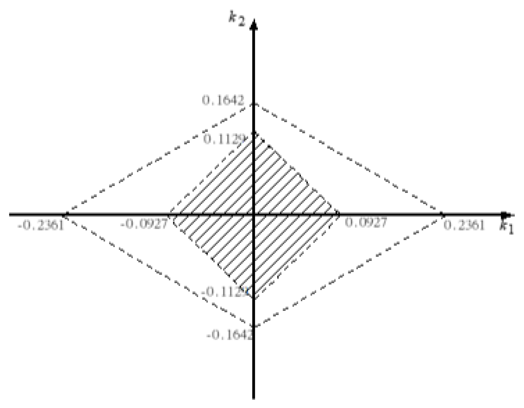
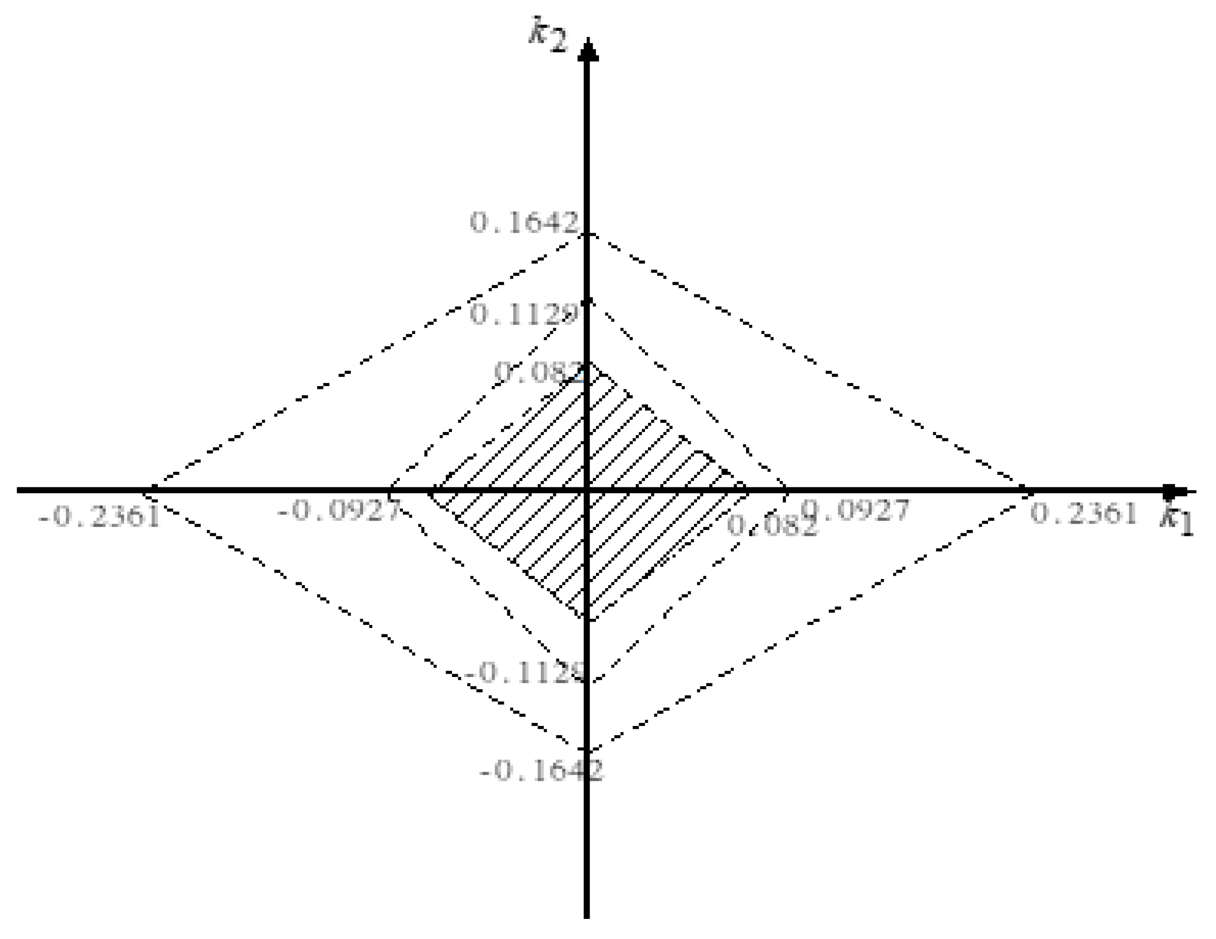
First, we can choose $L_i={\left[\begin{array}{cc}1& 1\end{array}\right]}^T$ such that ${\widehat{A}}_{ii}$ is stable, and matrices $P_{o1}=\left[\begin{array}{cc}0.7143& -0.2857\\ -0.2857& 0.6667\end{array}\right] \mathrm{and} P_{o2}=\left[\begin{array}{cc}0.2857& -0.1429\\ -0.1429& 0.5714\end{array}\right]$ can be also obtained. Hence, an observer of the system (17) for all ε∈(0, ∞) can be represented as below:

$$\begin{gathered} \left[\begin{array}{c}{\dot{\hat{x}}}_1^{\left(1\right)}\left(t\right)\\ {\dot{\hat{x}}}_1^{\left(2\right)}\left(t\right)\\ \epsilon {\dot{\hat{x}}}_2^{\left(1\right)}\left(t\right)\\ \epsilon {\dot{\hat{x}}}_2^{\left(2\right)}\left(t\right)\end{array}\right]=\left[\begin{array}{cccc}-1& 0& 0.2& 0.1\\ -0.5& -1.5& 0.3& 0\\ 0& 0.2& -3& -1\\ 0.3& 0.1& 0& -2\end{array}\right]\left[\begin{array}{c}{\hat{x}}_1^{\left(1\right)}\left(t\right)\\ {\hat{x}}_1^{\left(2\right)}\left(t\right)\\ {\hat{x}}_2^{\left(1\right)}\left(t\right)\\ {\hat{x}}_2^{\left(2\right)}\left(t\right)\end{array}\right]+\left[\begin{array}{cccc}1& 0& 0.5& 1\\ 2& 1& 0& 2\\ 0.5& 1& 0& 0\\ 0& 2& 0& 0\end{array}\right]\left[\begin{array}{c}{\hat{x}}_1^{\left(1\right)}\left(t\right)\\ {\hat{x}}_1^{\left(2\right)}\left(t\right)\\ {\hat{x}}_2^{\left(1\right)}\left(t\right)\\ {\hat{x}}_2^{\left(2\right)}\left(t\right)\end{array}\right]u\left(t\right)+\left[\begin{array}{c}1\\ 0.5\\ 1\\ 2\end{array}\right]u\left(t\right) \\ +\left[\begin{array}{c}1\\ 1\\ 1\\ 1\end{array}\right](y\left(t\right)-\left[\begin{array}{cccc}1& 0& 1& 0\end{array}\right]\left[\begin{array}{c}{\hat{x}}_1^{\left(1\right)}\left(t\right)\\ {\hat{x}}_1^{\left(2\right)}\left(t\right)\\ {\hat{x}}_2^{\left(1\right)}\left(t\right)\\ {\hat{x}}_2^{\left(2\right)}\left(t\right)\end{array}\right]) \end{gathered}$$

(21)

Second, according to Theorem 3, the six intersections, ${\overline{k}}_1=0.0927,$ ${\overline{k}}_2=0.1129,$ ${\widehat{k}}_1=0.2361,$ ${\widehat{k}}_2=0.1642$ and $\overline{k}=0.0927$ can be calculated from (16). Therefore, we conclude that system (17) can be stabilized by the following feedback control law for all ε∈(0, ∞):

$$u\left(t\right)=-\frac{k_1\left({\widehat{x}}_1^{\left(1\right)}+{\widehat{x}}_1^{\left(2\right)}\right)}{\sqrt{1+{({\widehat{x}}_1^{\left(1\right)}+{\widehat{x}}_1^{\left(2\right)})}^2}}-\frac{k_2\left({\widehat{x}}_2^{\left(1\right)}+{\widehat{x}}_2^{\left(2\right)}\right)}{\sqrt{1+{({\widehat{x}}_2^{\left(1\right)}+{\widehat{x}}_2^{\left(2\right)})}^2}}$$

(22)

where $k_1 \mathrm{and} k_2$ are selected inside the admissible region of the convex polygon, as shown in Figure 4.

4. Conclusions

According to the Lyapunov stability theorem, the designs of observer and observer-based stabilizers are presented for the singularly perturbed bilinear systems in this paper. The main advantage of this paper is that the whole $n_1+n_2$ dimensional process can be separated into two parts ($n_1$ and $n_2$ dimensional), which do not require the slow-fast decomposition. i.e., the main advantage of the proposed approach is that the whole dimensional design can be directly separated into two lower dimensions without the decomposition and composition of the slow and fast subsystems. Besides, this paper has three major contributions as well for the observer and controller design of the singularly perturbed bilinear systems. The first one is that the matrix $N_{22}=0$ is moved [18]. The second one is that the observer and closed-loop system are both stable for all ε∈(0, ∞), by those methods, the singular perturbation parameter is treated as a structured uncertainty. The last one is that we propose two different procedures for determining observer matrix $L_i$ and feedback gain $k_i$ in the structures of the observer (9) and the observer-based stabilizer (10), respectively.

References

- Mohler, R.R. Nonlinear Systems, Vol. II, Applications to Bilinear Control; Prentice Hall: Englewood Cliffs, NJ, USA, 1991. [Google Scholar]
- Wang, W.-J.; Chiou, J.-S. A non-linear control design for the discrete-time multi-input bilinear systems. Mechatronics 1991, 1, 87–94. [Google Scholar] [CrossRef]
- Benesty, J.; Paleologu, C.; Dogariu, L.-M.; Ciochină, S. Identification of Linear and Bilinear Systems: A Unified Study. Electronics 2021, 10, 1790. [Google Scholar] [CrossRef]
- Nie, Z.; Gao, F.; Yan, C.-B. A Multi-Timescale Bilinear Model for Optimization and Control of HVAC Systems with Consistency. Energies 2021, 14, 400. [Google Scholar] [CrossRef]
- Kokotovic, P.V.; Khalil, H.K.; O’Reilly, J. Singular Perturbation Methods in Control: Analysis and Design; Academic Press: London, UK, 1986. [Google Scholar]
- Naidu, D.S. Singular Perturbation Methodology in Control Systems; IEE and Perter Peregrinus: Stevenage Herts, UK, 1988. [Google Scholar]
- Chao, C.-T.; Chen, D.-H.; Chiou, J.-S. Stabilization and the Design of Switching Laws of a Class of Switched Singularly Perturbed Systems via the Composite Control. Mathematics 2021, 9, 1664. [Google Scholar] [CrossRef]
- Bobodzhanov, A.; Kalimbetov, B.; Safonov, V. Generalization of the Regularization Method to Singularly Perturbed Integro-Differential Systems of Equations with Rapidly Oscillating Inhomogeneity. Axioms 2021, 10, 40. [Google Scholar] [CrossRef]
- Liu, W.; Wang, Y.; Tian, Y. Feedback Stabilization for Discrete-Time Singularly Perturbed Systems via Limited Information with Data Packet Dropout. IEEE Access 2021, 9, 40585–40594. [Google Scholar] [CrossRef]
- Cerpa, E.; Prieur, C. Singular Perturbation Analysis of a Coupled System Involving the Wave Equation. IEEE Trans. Autom. Control 2020, 65, 4846–4853. [Google Scholar] [CrossRef]
- Song, J.; Niu, Y. Dynamic Event-Triggered Sliding Mode Control: Dealing with Slow Sampling Singularly Perturbed Systems. IEEE Trans. Circuits Syst. II Express Briefs 2020, 67, 1079–1083. [Google Scholar] [CrossRef]
- Dragan, V. On the Linear Quadratic Optimal Control for Systems Described by Singularly Perturbed Itô Differential Equations with Two Fast Time Scales. Axioms 2019, 8, 30. [Google Scholar] [CrossRef] [Green Version]
- Abdullazade, N.N.; Chechkin, G.A. Perturbation of the Steklov problem on a small part of the boundary. J. Math. Sci. 2014, 196, 441–450. [Google Scholar] [CrossRef]
- Borisov, D.I.; Cardone, G.; Checkhin, G.A.; Koroleva, Y.O. On elliptic operators with Steklov condition perturbed by Dirichlet condition on a small part of boundary. Calc. Var. Partial. Differ. Equ. 2021, 60, 1–44. [Google Scholar] [CrossRef]
- Chechkina, A.G. On singular perturbation of a Steklov-type problem with asymptotically degenerate spectrum. Dokl. Math. 2011, 84, 695–698. [Google Scholar] [CrossRef]
- Chechkina, A.G. Homogenization of spectral problems with singular perturbation of the Steklov condition. Izvestiya: Mathematics 2017, 81, 199–236. [Google Scholar] [CrossRef]
- Tzafestat, S.G.; Anagonostou, K.E. Stabilization of singularly perturbed strictly bilinear systems. IEEE Trans. Automat. Contr. 1984, 29, 943–946. [Google Scholar] [CrossRef]
- Asamoah, F.; Jamshidi, M. Stabilization of a class of singularly perturbed bilinear systems. Int. J. Contr. 1987, 46, 1589–1594. [Google Scholar] [CrossRef]
- Li, T.-H.S.; Sun, Y.-Y. Comments on: Stabilization of a class of singularly perturbed bilinear systems. Int. J. Contr. 1988, 48, 1357–1358. [Google Scholar] [CrossRef]
- Chiou, J.-S.; Kung, F.-C.; Li, T.-H.S. Robust stabilization of a class of singularly perturbed discrete bilinear systems. IEEE Trans. Automat. Contr. 2000, 45, 1187–1191. [Google Scholar] [CrossRef]
- Pan, S.-J.; Tsai, J.S.-H.; Pan, S.-T. Application of Genetic Algorithm on Observer-Based D-Stability Control for Discrete Multiple Time-Delay Singularly Perturbation Systems. Int. J. Innov. Comput. Inf. Control 2011, 7, 3345–3358. [Google Scholar]
- Zhou, K.; Khargonekar, P.P. Robust stabilization of linear systems with norm-bounded time-varying uncertainty. Sys. Control Lett. 1988, 10, 17–20. [Google Scholar] [CrossRef]
- Saydy, L. New stability/performance results for singularly perturbed system. Automatica 1996, 32, 807–818. [Google Scholar] [CrossRef]
- Longchamp, R. Controller design for bilinear systems. IEEE Trans. Automat. Control 1980, 25, 547–548. [Google Scholar] [CrossRef]
- Genesio, R.; Tesi, A. The output stabilization of SISO bilinear systems. IEEE Trans. Automat. Control 1988, 33, 950–952. [Google Scholar] [CrossRef]
- Benallou, A.; Mellichamp, D.A.; Seborg, D.E. Optimal stabilizing controllers for bilinear systems. Int. J. Control 1988, 48, 1487–1501. [Google Scholar] [CrossRef]
- Hara, S.; Fumta, K. Minimal order state observers for bilinear systems. Int. J. Control 1976, 24, 705–718. [Google Scholar] [CrossRef]
- Funahashi, Y. Stable state estimator for bilinear system. Int. J. Control 1979, 29, 181–188. [Google Scholar] [CrossRef]
- Derese, I.; Noldus, E.J. Existence of bilinear state observers for bilinear system. IEEE Trans. Automat. Control 1981, 26, 590–592. [Google Scholar] [CrossRef]
- Derse, I.; Stevens, P.; Noldus, E.J. Observers for bilinear systems with bounded input. Int. J. Syst. Sci. 1979, 10, 649–668. [Google Scholar] [CrossRef]
Publisher’s Note: MDPI stays neutral with regard to jurisdictional claims in published maps and institutional affiliations. |
© 2021 by the authors. Licensee MDPI, Basel, Switzerland. This article is an open access article distributed under the terms and conditions of the Creative Commons Attribution (CC BY) license (https://creativecommons.org/licenses/by/4.0/).
Share and Cite
Chen, D.-H.; Chao, C.-T.; Chiou, J.-S. Robust Stabilization and Observer-Based Stabilization for a Class of Singularly Perturbed Bilinear Systems. Mathematics 2021, 9, 2380. https://doi.org/10.3390/math9192380
Chen D-H, Chao C-T, Chiou J-S. Robust Stabilization and Observer-Based Stabilization for a Class of Singularly Perturbed Bilinear Systems. Mathematics. 2021; 9(19):2380. https://doi.org/10.3390/math9192380
Chicago/Turabian StyleChen, Ding-Horng, Chun-Tang Chao, and Juing-Shian Chiou. 2021. "Robust Stabilization and Observer-Based Stabilization for a Class of Singularly Perturbed Bilinear Systems" Mathematics 9, no. 19: 2380. https://doi.org/10.3390/math9192380
APA StyleChen, D.-H., Chao, C.-T., & Chiou, J.-S. (2021). Robust Stabilization and Observer-Based Stabilization for a Class of Singularly Perturbed Bilinear Systems. Mathematics, 9(19), 2380. https://doi.org/10.3390/math9192380