Evolutionary Derivation of Runge–Kutta Pairs of Orders 5(4) Specially Tuned for Problems with Periodic Solutions

Abstract

The purpose of the present work is to construct a new Runge–Kutta pair of orders five and four to outperform the state-of-the-art in these kind of methods when addressing problems with periodic solutions. We consider the family of such pairs that the celebrated Dormand–Prince pair also belongs. The chosen family comes with coefficients that all depend on five free parameters. These latter parameters are tuned in a way to furnish a new method that performs best on a couple of oscillators. Then, we observe that this trained pair outperforms other well known methods in the relevant literature in a standard set of problems with periodic solutions. This is remarkable since no special property holds such as high phase-lag order or an extended interval of periodicity.

1. Introduction

The Initial Value Problem (IVP) is

$$y^{\prime }=f(x,y),y\left(x_0\right)=y_0$$

(1)

with $x_0\in \mathbb{R}$ and the vectors $y,y^{\prime }\in {\mathbb{R}}^m$. The function f is defined as $f:\mathbb{R}\times {\mathbb{R}}^m\to {\mathbb{R}}^m.$

Runge–Kutta (RK) pairs are perhaps the most used numerical methods for addressing (1). They usually presented in a so-called Butcher tableau [1,2] as given below.

$$\begin{array}{rr}c& A\\ \hfill & b\\ \hfill & \widehat{b}\end{array}$$

In this type of tableau, we have $b^T,{\widehat{b}}^T,c\in {\mathbb{R}}^s$ while $A\in {\mathbb{R}}^{s\times s}.$ Then, the method shares s stages and in case that A is strictly lower triangular, it is evaluated explicitly. The numerical approximations of the solution step from $(x_n,y_n)\in {\mathbb{R}}^{1+m}$ to $x_{n+1}=x_n+h_n$ by producing two numerical estimations for $y\left(x_{n+1}\right).$ Namely, $y_{n+1}\in {\mathbb{R}}^m$ and ${\widehat{y}}_{n+1}\in {\mathbb{R}}^m$, given by

$$y_{n+1}=y_n+h_n\sum _{i=1}^s{b}_i{f}_i,$$

and

$${\widehat{y}}_{n+1}=y_n+h_n\sum _{i=1}^s{\widehat{b}}_i{f}_i,$$

with

$$f_i=f(x_n+c_i{h}_n,y_n+h_n\sum _{j=1}^{i-1}{a}_{ij}{f}_j),$$

for $i=1,2,\cdots ,s.$ These two approximations $y_{n+1}\in {\mathbb{R}}^m$ and ${\widehat{y}}_{n+1}\in {\mathbb{R}}^m$ are of algebraic orders p and $q<p$, respectively. This means that when expanding them in Taylor series, they attain orders $O\left(h^p\right)$ and $O\left(h^q\right)$, respectively, with h being the proper step–length. Then, a local error estimation

$${ϵ}_n=h_n^{p-q-1}·{\parallel y_{n+1}-{\widehat{y}}_{n+1}\parallel }_{\infty },$$

is formed in every step and is combined in an algorithm for changing the steplength.

$$h_{n+1}=0.8·h_n^{}·{\left(\frac{t}{{ϵ}_n}\right)}^{1/p},$$

with t a small positive number which is set by the user and is named tolerance. The safety factor $0.8$ is in common use in such formulas and offers increased reliability to the results. Whenever ${ϵ}_n<t$, we use the above formula for defining the length of the next step forward. In reverse, when ${ϵ}_n\ge t$ we again use it without advancing the solution in this case and using instead the value $h_{n+1}$ as a new trial step $h_n$. Information in the issue can be found with details in  [3]. As an abbreviation these methods are named RKp(q) airs.

Carl David Tolmé Runge [4] and Martin Wilhelm Kutta [5] introduced the methods bearing their names almost in the turning of the 19th century. For almost 60 years the these methods were implemented with constant step sizes. Richardson extrapolation appeared in the meantime [6] and was used in a kind of step control through doubling and halving [7]. Runge–Kutta pairs appeared 60 years ago. The first series of well-known Runge–Kutta pairs of orders 5(4), 6(5), and 8(7) were presented by Fehlberg [8,9]. In the early 1980s, Dormand and Prince gave their celebrated pairs [10,11].

Non-stiff problems having the form (1) are well suited for being efficiently solved by Runge–Kutta pairs. There is a number of different pairs sharing various orders. We may explain this by the accuracy on demand. Thus, the lesser the accuracy required, the lesser order pairs are chosen. Otherwise, for stringent accuracies at quadruple precision, a high order pair has to be preferred.

Here, we concentrate on RK5(4) pairs which are the first choice when middle tolerances are used. Our special interest is in problems of the form (1) with periodic/oscillatory solutions. In the following, we focus on producing a RK5(4) pair that best address the latter type of problems.

The paper is organized in sections as follows.

• Introduction
• Theory of Runge–Kutta pairs for orders 5(4)
• Training the coefficients
• Numerical tests
• Conclusions

2. Theory of Runge–Kutta Pairs for Orders 5(4)

Runge–Kutta pairs of orders five and four are perhaps the most used ones. The coefficients of these pairs have to satisfy 25 order conditions when the almost obligatory

$$A·e=c,e=[1,1,\cdots ,1]\in {\mathbb{R}}^s$$

(2)

holds. Namely, 17 order conditions for the higher order formula and another 8 conditions for the fourth order formula. For a seven stages (i.e., $s=7$) pair with an FSAL (First Stage As Last) property there are 28 coefficients after considering (2). Over the years, various techniques for solving this system have been presented. The solutions form different families. Dormand and Prince presented such a family and perhaps the most famous pair of all in [10]. Papakostas and Papageorgiou studied this family extensively [12]. Then, we may choose arbitrarily the coefficients $c_2,c_3,$$c_4,$$c_5,$${\widehat{b}}_7$ and produce all the rest coefficients explicitly. The particular pair DP5(4) appeared in [10] shares small principal truncation error coefficients and it is implemented in the builtin function ode45 of MATLAB [13].

We now proceed presenting explicit formulas for the remaining coefficients that only depend on the five free parameters.

$$b_3=\frac{c_4(5-10c_5)+5c_5-3}{60(c_3-1)c_3(c_3-c_4)(c_3-c_5)},b_4=\frac{5c_3(2c_5-1)-5c_5+3}{60(c_4-1)c_4(c_3-c_4)(c_4-c_5)},$$

$$\begin{array}{ccc}\hfill b_5& =& \frac{5c_3(2c_4-1)-5c_4+3}{60(c_5-1)c_5(c_3-c_5)(c_5-c_4)},\hfill \\ \hfill b_6& =& \frac{5c_3(c_4(6c_5-4)-4c_5+3)-20c_4{c}_5+15c_4+15c_5-12}{60(c_3-1)(c_4-1)(c_5-1)},\hfill \end{array}$$

$${\widehat{b}}_3=\frac{\left(\begin{array}{c}\frac{\left(\begin{array}{c}10(6{\widehat{b}}_7-1)c_3^2{c}_4\\ +c_3(-8{\widehat{b}}_7(7c_4+1)\\ +8c_4+1)+2(8{\widehat{b}}_7-1)c_4\end{array}\right)\left(\begin{array}{c}5c_3(c_4(6c_5-4)-4c_5+3)\\ -20c_4{c}_5+15c_4+15c_5-12\end{array}\right)}{5\left(c_3-1\right)\left(\begin{array}{c}10c_3^2{c}_4\\ -c_3(8c_4+1)+2c_4\end{array}\right)}\\ -12{\widehat{b}}_7(c_4-1)(c_5-1)+2c_4(3c_5-2)-4c_5+3\end{array}\right)}{12c_3(c_3-c_4)(c_3-c_5)},$$

$${\widehat{b}}_4=\frac{\left(\begin{array}{c}-\frac{\left(\begin{array}{c}10(6{\widehat{b}}_7-1)c_3^2{c}_4\\ +c_3(-8{\widehat{b}}_7(7c_4+1)+8c_4+1)\\ +2(8{\widehat{b}}_7-1)c_4\end{array}\right)\left(\begin{array}{c}5c_3(c_4(6c_5-4)-4c_5+3)\\ -20c_4{c}_5+15c_4+15c_5-12\end{array}\right)}{5(c_4-1)\left(\begin{array}{c}10c_3^2{c}_4\\ -c_3(8c_4+1)+2c_4\end{array}\right)}\\ +12{\widehat{b}}_7(c_3-1)(c_5-1)-2c_3(3c_5-2)+4c_5-3\end{array}\right)}{12c_4(c_3-c_4)(c_4-c_5)},$$

$${\widehat{b}}_5=\frac{\left(\begin{array}{c}\left\{\frac{\left(\begin{array}{c}10(6{\widehat{b}}_7-1)c_3^2{c}_4\\ +c_3(-8{\widehat{b}}_7(7c_4+1)+8c_4+1)\\ +2(8{\widehat{b}}_7-1)c_4\end{array}\right)\left(\begin{array}{c}5c_3(c_4(6c_5-4)-4c_5+3)\\ -20c_4{c}_5+15c_4+15c_5-12\end{array}\right)}{5(c_5-1)\left(\begin{array}{c}10c_3^2{c}_4\\ -c_3(8c_4+1)+2c_4\end{array}\right)}\right\}\\ -12{\widehat{b}}_7(c_3-1)(c_4-1)+2c_3(3c_4-2)-4c_4+3\end{array}\right)}{12c_5(c_3-c_5)(c_4-c_5)},$$

$${\widehat{b}}_6=-\frac{\left\{\begin{array}{c}\left(10(6{\widehat{b}}_7-1)c_3^2{c}_4+c_3(-8{\widehat{b}}_7(7c_4+1)+8c_4+1)+2(8{\widehat{b}}_7-1)c_4\right)·\\ (5c_3(c_4(6c_5-4)-4c_5+3)-20c_4{c}_5+15c_4+15c_5-12)\end{array}\right\}}{60(c_3-1)(c_4-1)(c_5-1)\left(10c_3^2{c}_4-c_3(8c_4+1)+2c_4\right)},$$

$$a_{3,2}=\frac{c_3^2}{2c_2},a_{4,2}=\frac{c_4^2(3c_3-2c_4)}{2c_2{c}_3},a_{4,3}=\frac{c_4^2(c_4-c_3)}{c_3^2},$$

$$a_{5,2}=\frac{c_5\left(15c_3^2{c}_4(2c_5-1)+c_3\left(c_4\left(6-20c_5^2\right)+(3-5c_5)c_5\right)+2c_4{c}_5(5c_5-3)\right)}{2c_2{c}_3(5c_3(2c_4-1)-5c_4+3)},$$

$$a_{5,3}=-\frac{c_5(c_3-c_5)\left(10c_3^2{c}_4(2c_5-1)+c_3\left(\begin{array}{c}-5c_4^2(4c_5-3)\\ +c_4(4-15c_5)+2c_5\end{array}\right)+2c_4^2(5c_5-3)\right)}{2c_3^2(c_3-c_4)(5c_3(2c_4-1)-5c_4+3)},$$

$$a_{5,4}=\frac{(5c_3-2)c_5(c_3-c_5)(c_4-c_5)}{2c_4(c_3-c_4)(5c_3(2c_4-1)-5c_4+3)},$$

$$a_{6,2}=\frac{15c_3^2{c}_4(2c_5-1)+c_3(c_4(16-30c_5)-5c_5+3)+2c_4(5c_5-3)}{2c_2{c}_3(5c_3(c_4(6c_5-4)-4c_5+3)-20c_4{c}_5+15c_4+15c_5-12)},$$

$$a_{6,3}=-\frac{(c_3-1)·\left(\begin{array}{c}-c_3^2\left(5c_4^2(4c_5-3)+20c_4{c}_5^2+c_4-2\right)\\ +c_3\left(c_4^2(25c_5-16)+c_4\left(40c_5^2-45c_5+16\right)-2\left(5c_5^2-7c_5+3\right)\right)\\ 10c_3^3{c}_4(2c_5-1)+2c_4^2(3-5c_5)c_5\end{array}\right)}{2c_3^2(c_3-c_4)(c_3-c_5)(5c_3(c_4(6c_5-4)-4c_5+3)-20c_4{c}_5+15c_4+15c_5-12)},$$

$$a_{6,4}=\frac{(c_3-1)(c_4-1)\left(5c_3\left(c_4-4c_5^2+5c_5-2\right)-2\left(c_4-5c_5^2+7c_5-3\right)\right)}{2c_4(c_3-c_4)(c_4-c_5)(5c_3(c_4(6c_5-4)-4c_5+3)-20c_4{c}_5+15c_4+15c_5-12)},$$

$$a_{6,5}=\frac{(c_3-1)(c_4-1)(c_5-1)(5c_3(2c_4-1)-5c_4+3)}{c_5(c_3-c_5)(c_4-c_5)(5c_3(c_4(6c_5-4)-4c_5+3)-20c_4{c}_5+15c_4+15c_5-12)},$$

$$b_1=1-b_3-b_4-b_5-b_6,{\widehat{b}}_1=1-{\widehat{b}}_3-{\widehat{b}}_4-{\widehat{b}}_5-{\widehat{b}}_6-{\widehat{b}}_7,$$

$$a_{21}=c_2,a_{31}=c_3-a_{32},a_{41}=c_4-a_{42}-a_{43},$$

$$a_{51}=c_5-a_{52}-a_{53}-a_{54},a_{61}=c_6-a_{62}-a_{63}-a_{64}-a_{65},$$

and finally the FSAL property holds

$$a_{7j}=b_j,j=1,2,\cdots ,6.$$

This means that although $s=7,$ the method wastes only six stages per step and the seventh stage is reused as first stage of the next step.

The question raising now is how to choose the free parameters. Traditionally, the method developers try to minimize some norm for the principal term of the local truncation error, i.e., the terms of $h^6$ in the residual of Taylor error expansions corresponding to the fifth order method of the underlying RK pair. Another choice is to increase the phase-lag order. This means that we try to reduce the gap in the angle among the numerical and the theoretical solution in a free oscillator [14]. The latter approach is well suited for usage in problems with periodic solutions.

3. Training the Coefficients

We intent to derive a particular RK5(4) pair that belongs to the family discussed above. The resulting pair has to perform best on harmonic oscillators and other problems with periodic solutions. For achieving this, we will first try to find a pair that performs best on a couple of harmonic oscillators. Then, we will check if this performance expands to other problems with periodic solutions.

Thus, we concentrate on the harmonic oscillator

$$y^{″}=-{\mu }^{2}y,y\left(0\right)=1,y^{\prime }\left(0\right)=0,x\in [0,10\pi ],$$

with theoretical solution $y\left(x\right)=cos\mu x$. This problem can be transformed to a first-order system,

$$\left[\begin{array}{c}{y}_1^{\prime }\\ y_2^{\prime }\end{array}\right]\left[\begin{array}{cc}0\hfill & 1\hfill \\ -{\mu }^2\hfill & 0\hfill \end{array}\right]\left[\begin{array}{c}{y}_1\\ y_2\end{array}\right],y_1\left(0\right)=1,y_2\left(0\right)=0,x\in [0,10\pi ],$$

and then solved it numerically by a RK5(4) pair picked from the family of solutions we are concerned here. We use tolerance $t={10}^{-11}$ and $\mu =3$ and $\mu =7$. The choice of $\mu$ is tailored by the numerical tests we will present below. The values selected are best placed when $\mu \in [0,10]$. Notice that the above selection of $\mu$ is for the training phase. It is hoped that the resulted method will furnish better results for every $\mu$.

We record the number $k_1$ and $k_2$ of stages (i.e., function evaluations) needed and the global errors $g_1$ and $g_2$ observed over the grid (mesh) in the interval of integration, respectively (i.e for both selections of $\mu$). Then, we form two efficiency measures

$$u_j=k_j·g_j^{1/5},j=1,2$$

(3)

in the sense that higher values mean lower efficiency. These measures were introduced in [15] for comparing pairs of the same order.

Now we may set as fitness function the sum $u_1+u_2$ which is meant to be minimized. Thus, the fitness function consists of two runs of an Initial Value Problem. The value $u_1+u_2$ changes according to the selection of the free parameters $c_2,c_3,$$c_4,$$c_5$, and ${\widehat{b}}_7.$ We actually do not care at this stage for ${\widehat{b}}_7$, as this coefficient actually affects only the tolerance. Indeed we may choose

$${\tilde{b}}_7=\lambda ·{\widehat{b}}_7,\lambda \ne 0,$$

and set a new $\tilde{b}=\lambda \widehat{b}+(1-\lambda )b,$ as the new fourth order formula. Then, the tolerance simply becomes $\lambda t.$

This idea was originally appeared in [16]. Here, for the minimization of $u_1+u_2$ we tried Differential Evolution [17]. We have already got positive results using this approach for methods in integrating of orbits [18,19]. In these latter works, we trained the coefficients of the methods on a Kepler orbit. Then we observed very pleasant results over a set of Kepler orbits as long on other known orbital problems.

DE is an iterative procedure and in every iteration, named generation g, we work with a “population” of individuals ${\left(c_2^{\left(g\right)},c_3^{\left(g\right)},c_4^{\left(g\right)},c_5^{\left(g\right)},{\widehat{b}}_7^{\left(g\right)}\right)}_i$, $i=1,2,\cdots ,P$ with P the population size. An initial population ${\left(c_2^{\left(0\right)},c_3^{\left(0\right)},c_4^{\left(0\right)},c_5^{\left(0\right)},{\widehat{b}}_7^{\left(0\right)}\right)}_i$, $i=1,2,\cdots ,P$ is randomly created in the first step of the method. We have also set as fitness function the measure $u_1+u_2$ obtained after two runs of harmonic oscilator. The fitness function is then evaluated for each individual in the initial population. In each generation (iteration) g, a three-phase sequential scheme updates all of the individuals involved. These phases are Differentiation, Crossover, and Selection. For further details in the issue see in [20]. We used MATLAB Software DeMat [21] for implementing the latter technique.

The optimization furnished five values for the parameters. The result is rather robust, i.e., we get almost the same optimal value for u even for neighboring parameters. Thus, we present the selected parameters in 6 significant decimal digits below,

$$c_2=\frac{6618}{21991},c_3=\frac{3679}{11497},c_4=\frac{25691}{30789},c_5=\frac{5444}{5589},{\widehat{b}}_7=\frac{11}{400}.$$

The resulting pair is presented in Table 1.

Table 1. Coefficients of NEW5(4) pair, accurate for double precision computations.

0
$\frac{6618}{21991}$	$\frac{6618}{21991}$
$\frac{3679}{11497}$	$\frac{105068699}{701077884}$	$\frac{87461119}{514086615}$
$\frac{25691}{30789}$	$-\frac{156758655}{1553593837}$	$-\frac{1971428717}{769326967}$	$\frac{1150666171}{328963002}$
$\frac{5444}{5589}$	$-\frac{492306695}{897757177}$	$-\frac{4668023671}{453052236}$	$\frac{11886685592}{971735195}$	$-\frac{563000739}{1384986010}$
1	$-\frac{1277080003}{2297156422}$	$-\frac{19858667372}{1842147371}$	$\frac{12595531818}{990040061}$	$-\frac{479293713}{1359193574}$	$-\frac{43409699}{1295767884}$
1	$\frac{118291366}{1206413123}$	0	$\frac{224782023}{473511539}$	$\frac{563088416}{949003535}$	$-\frac{735589742}{998947995}$	$\frac{326830465}{573133003}$
5th-order	$\frac{118291366}{1206413123}$	0	$\frac{224782023}{473511539}$	$\frac{563088416}{949003535}$	$-\frac{735589742}{998947995}$	$\frac{326830465}{573133003}$
4th-order	$\frac{34973117}{364942645}$	0	$\frac{660068138}{1367732753}$	$\frac{376526469}{703576622}$	$-\frac{319022417}{656211193}$	$\frac{219368109}{635728846}$	$\frac{11}{400}$

For the above selection of free parameters, we got

$$u_1^{\mathrm{NEW}54}=88.37,u_2^{\mathrm{NEW}54}=284.89,$$

while for DP5(4) we observed

$$u_1^{\mathrm{DP}54}=279.28,u_2^{\mathrm{DP}54}=797.55$$

i.e.,

$$\frac{u_1^{\mathrm{DP}54}}{u_1^{\mathrm{NEW}54}}+\frac{u_2^{\mathrm{DP}54}}{u_2^{\mathrm{NEW}54}}=\frac{279.28}{88.37}+\frac{797.55}{284.89}\approx 3.16+2.80=5.96,$$

meaning that DP5(4) is $216\%$ (interpreting number $3.16$) and $180\%$ (interpreting number $2.80$), respectively, more expensive for delivering the same accuracy in the two oscillators chosen above.

The Euclidean norm of the principal truncation error coefficients for the new pair is $\parallel T^{\left(6\right)}{\parallel }_2\approx 2.82\times {10}^{-4}$ which is a little smaller than the corresponding value $\parallel T^{\left(6\right)}{\parallel }_2\approx 3.99\times {10}^{-4}$ for DP5(4). The absolute stability interval is $(-3.55,0]$ which is rather in normal magnitude. No extra phase-lag order is observed as $b{A}^{4}c=\frac{13128101}{9439496880}\ne \frac{1}{840}$. See in [14] for details on phase-lag property.

In conclusion, it seems that no extra property is present. The new pair appeared in Table 1 does not possess something interesting. It is hard to believe its special performance after seeing its traditional characteristics.

Other authors have also tried recently to train coefficients of RK methods [22]. However, in that later paper, only second- and third-order methods are considered [4,5] with constant step sizes and over single problems (e.g., Van der Pol). The learning algorithm given there remains to be tested on current and stiffer cases. Our proposal for Differential evolution comes after several papers through the years [16].

4. Numerical Tests

We tested the following two pairs chosen from the family studied above.

• DP5(4) pair given in [10].
• NEW5(4) pair given here in Table 1.

DP5(4) has proven over the years to be perhaps the best pair of orders five and four. Other pairs also exist but the difference with DP5(4) is very small. We do not consider pairs that exploit the knowledge of frequency since this property is not considered here.

All the pairs were run for tolerances ${10}^{-5},{10}^{-6},\cdots ,{10}^{-11},$ and the efficiency measures of the form (3) were recorded. Notice that actually all the problems are transformed in systems of first order equations.

The problems we tested are the following.

1–5. The model problem

$$y^{″}\left(x\right)=-{\mu }^{2}y\left(x\right),y\left(0\right)=1,y^{\prime }\left(0\right)=0,x\in [0,10\pi ],$$

with theoretical solution $y\left(x\right)=cos\left(\mu x\right)$. This problem was run for five different selections of $\mu$. Thus, when we use $\mu =1$ the problem is numbered as 1st problem. Then we choose $\mu =3$ and the problem is numbered as 2nd problem. In consequence when $\mu =5$ the problem is numbered as 3rd problem, when $\mu =7$ the problem is numbered as 4th problem, and when $\mu =9$ the problem is numbered as 5th problem.

6. The inhomogeneous problem

$$y^{″}\left(x\right)=-100y\left(x\right)+99sinx,y\left(0\right)=1,y^{\prime }\left(0\right)=11,x\in [0,10\pi ],$$

with theoretical solution $y\left(x\right)=cos\left(10x\right)+sin\left(10x\right)+sinx$.

7. The Bessel equation

The well-known Bessel equation

$$y^{″}\left(x\right)=-y\left(x\right)·\frac{1+400x^2}{4x^2},$$

is verified by a theoretical solution of the form [14]

$$y\left(x\right)=J_0\left(10x\right)·\sqrt{x},$$

with $J_0$ the zeroth order Bessel function of the first kind. This equation in also integrated in the interval $[0,10\pi ]$.

8. The Duffing equation

Next, we choose the equation

$$\begin{array}{ccc}\hfill y^{″}\left(x\right)& =& \frac{1}{500}·cos(1.01x)-y\left(x\right)-y{\left(x\right)}^3,\hfill \\ \hfill y\left(0\right)& =& 0.2004267280699011,y^{\prime }\left(0\right)=0,\hfill \end{array}$$

with an approximate analytical solution given in [23],

$$y\left(x\right)\approx \left\{\begin{array}{c}6·{10}^{-16}cos\left(11.11x\right)+4.609·{10}^{-13}cos\left(9.09x\right)\hfill \\ +3.743495·{10}^{-10}cos\left(7.07x\right)+3.040149839·{10}^{-7}cos\left(5.05x\right)\hfill \\ +2.469461432611·{10}^{-4}cos\left(3.03x\right)0.2001794775368452cos\left(1.01x\right)\hfill \end{array}\right\}$$

We again solved the above equation in the interval $\left[0,10\pi \right]$.

9. semi-Linear system.

The nonlinear problem proposed by Franco and Gomez [24] follows.

$$\begin{array}{ccc}\hfill y^{″}\left(t\right)& =& \left(\begin{array}{cc}-199& -198\\ 99& 98\end{array}\right)·y(x)+\left(\begin{array}{}{(y_1+y_2)}^2+{sin}^2(10x)-1\\ {(y_1+2y_2)}^2-{10}^{-6}sin{}^2(x)\end{array}\right),\hfill \\ \hfill x& \in & [0,10\pi ],\hfill \end{array}$$

with theoretical solution

$$y(t)=\left(\begin{array}{c}2cos\left(10x\right)-{10}^{-3}sin\left(x\right)\\ -cos\left(10x\right)+{10}^{-3}sin\left(x\right)\end{array}\right).$$

10. Van der Pol oscillator.

The equation we solved is

$$y^{″}=0.1·(1-y{\left(x\right)}^2)y^{\prime }\left(x\right)-y\left(x\right),y\left(0\right)=-0.2,y^{\prime }\left(0\right)=0,x\in [0,10\pi ],$$

and no analytical solution is known. Thus, the error at grid was estimated using an eighth-order pair from [25] at tolerance ${10}^{-14}$.

We calculated seventy (i.e., 7 tolerances times 10 problems) efficiency measures for each pair. We set NEW54 as the reference pair. Then, we divide each efficiency measure of DP5(4) with the corresponding efficiency measure of NEW5(4). The results are recorded in Table 2. The two underlined numbers correspond to the ratios found in the phase of training above as the training was done for problems 2 and 4 and tolerance ${10}^{-11}$. Numbers greater than 1 are in favor of the second pair. ${\widehat{b}}_7$ was chosen so that the total function evaluations spend for both pairs over all 70 runs is almost equal. The rightmost column shows the mean over all tolerances for each problem. The overall average observed ratio is $1.85$ meaning that DP5(4) is about $85\%$ more expensive. This is quite remarkable since much effort has been put over the years for achieving even 10–20% of efficiency [25]. In reverse, this means that about ${log}_{10}1.{85}^5\approx 1.34$ digits were gained in average at the same costs [15].

Table 2. Efficiency measures ratios of DP5(4) vs. NEW5(4) over the interval $[0,10\pi ]$.

	Tolerances
Problem	${\mathbf{10}}^{-\mathbf{5}}$	${\mathbf{10}}^{-\mathbf{6}}$	${\mathbf{10}}^{-\mathbf{7}}$	${\mathbf{10}}^{-\mathbf{8}}$	${\mathbf{10}}^{-\mathbf{9}}$	${\mathbf{10}}^{-\mathbf{10}}$	${\mathbf{10}}^{-\mathbf{11}}$	Mean
1	$1.33$	$1.45$	$1.60$	$1.76$	$1.93$	$2.12$	$2.65$	$1.83$
2	$1.36$	$1.48$	$1.63$	$1.79$	$1.96$	$2.17$	$\underline{3.16}$	$1.94$
3	$1.37$	$1.50$	$1.64$	$1.80$	$1.98$	$2.20$	$2.74$	$1.89$
4	$1.38$	$1.51$	$1.65$	$1.81$	$1.99$	$2.22$	$\underline{2.80}$	$1.91$
5	$1.39$	$1.51$	$1.66$	$1.82$	$1.99$	$2.23$	$2.24$	$1.83$
6	$1.41$	$1.54$	$1.68$	$1.85$	$2.02$	$2.35$	$1.75$	$1.80$
7	$1.32$	$1.44$	$1.57$	$1.72$	$1.89$	$2.08$	$2.67$	$1.81$
8	$1.14$	$1.4$	$1.65$	$1.93$	$2.19$	$2.38$	$2.40$	$1.87$
9	$1.52$	$1.67$	$1.84$	$2.00$	$2.17$	$2.54$	$1.98$	$1.96$
10	$1.25$	$1.36$	$1.49$	$1.62$	$1.77$	$1.94$	$2.24$	$1.67$

Because of the problems used for training, it is obvious that we expect better results when there is a larger linear part and a smaller nonlinear part. However, NEW5(4) outperformed DP5(4) even in the clearly nonlinear problems. We also mention that we got more or less similar results for longer integrations. Especially the results for the interval $[0,20\pi ]$ are shown in Table 3. The overall average observed is $1.84$ and the results slightly differ from those of the previous Table.

Table 3. Efficiency measures ratios of DP5(4) vs. NEW5(4) over the interval $[0,20\pi ]$.

	Tolerances
Problem	${\mathbf{10}}^{-\mathbf{5}}$	${\mathbf{10}}^{-\mathbf{6}}$	${\mathbf{10}}^{-\mathbf{7}}$	${\mathbf{10}}^{-\mathbf{8}}$	${\mathbf{10}}^{-\mathbf{9}}$	${\mathbf{10}}^{-\mathbf{10}}$	${\mathbf{10}}^{-\mathbf{11}}$	Mean
1	$1.33$	$1.45$	$1.60$	$1.75$	$1.92$	$2.11$	$2.64$	$1.83$
2	$1.36$	$1.49$	$1.63$	$1.78$	$1.96$	$2.16$	$3.17$	$1.94$
3	$1.37$	$1.50$	$1.64$	$1.80$	$1.97$	$2.18$	$2.58$	$1.86$
4	$1.38$	$1.51$	$1.65$	$1.81$	$1.98$	$2.19$	$2.79$	$1.90$
5	$1.39$	$1.51$	$1.66$	$1.82$	$1.99$	$2.23$	$2.42$	$1.86$
6	$1.41$	$1.54$	$1.68$	$1.85$	$2.03$	$2.36$	$1.80$	$1.81$
7	$1.32$	$1.44$	$1.57$	$1.72$	$1.89$	$2.07$	$2.65$	$1.81$
8	$1.08$	$1.36$	$1.66$	$1.98$	$2.33$	$2.58$	$2.58$	$1.94$
9	$1.52$	$1.67$	$1.84$	$2.00$	$2.17$	$2.44$	$1.73$	$1.91$
10	$1.24$	$1.28$	$1.34$	$1.44$	$1.58$	$1.75$	$2.17$	$1.54$

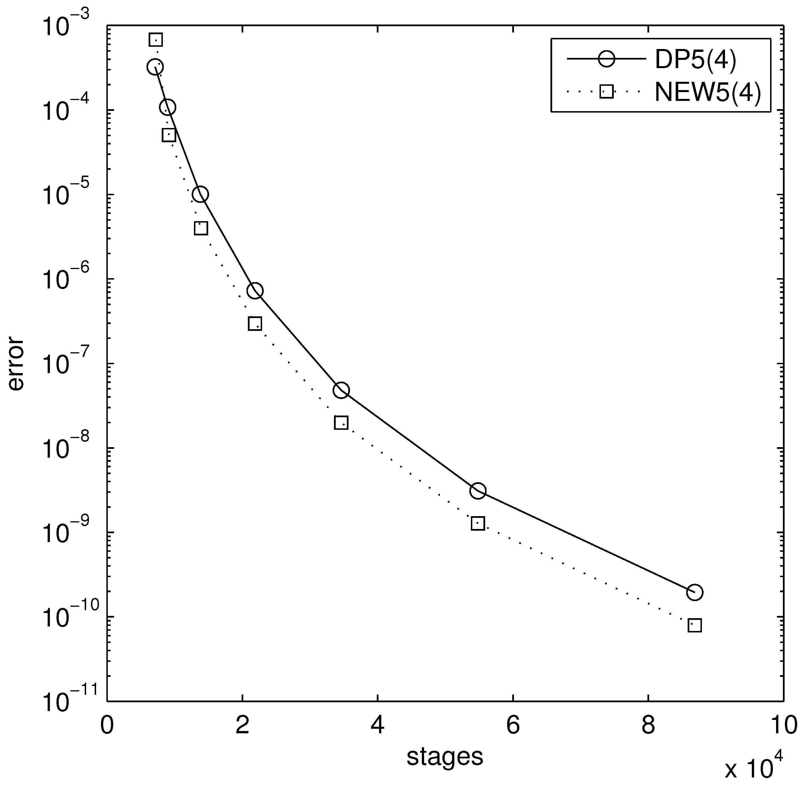
As a final test, we included a more challenging problem which appears frequently in similar works [14,23], namely, the hyperbolic PDE,

$$\begin{array}{ccc}\hfill \frac{\vartheta u}{\vartheta x}& =& \frac{\vartheta u}{\vartheta r},u(x,0)=0,u(0,r)=sin{\pi }^2{r}^2,\hfill \\ \hfill 0& \le & r\le 1,x\ge 0,\hfill \end{array}$$

is discretized by symmetric differences (with $\Delta r=1/50$) to the system of ODEs

$$\left[\begin{array}{c}{y}_1^{\prime }\hfill \\ y_2^{\prime }\hfill \\ \\ \\ y_{50}^{\prime }\hfill \end{array}\right]=\frac{1}{2}·\frac{1}{(1/50)}\left[\begin{array}{ccccc}0\hfill & -1\hfill & & & \\ 1\hfill & 0\hfill & -1\hfill & & \\ & & & & \\ & & 1\hfill & 0\hfill & -1\hfill \\ & & -1\hfill & 4\hfill & -3\hfill \end{array}\right]·\left[\begin{array}{c}{y}_1\hfill \\ y_2\hfill \\ \\ \\ y_{50}\hfill \end{array}\right].$$

The 500th zero of the 20th component in the above problem is reached for

$$x_{500}=33.50999699533,$$

which is found by a very accurate integration at stringent tolerances. We integrated the methods to that point. The results presented as stages vs. error in a semi-log form and are given in Figure 1.

Figure 1. Results of DP5(4) vs. NEW5(4) for the Hyperbolic PDE.

The results are very promising. Some future research may use optimization on a wider range of tolerances and model problems. Perhaps a pair spending a parameter for fulfilling the phase-lag property and then trained for periodic problems would furnish even more interesting results. Of course, application of this technique on other classes of problems is also possible, e.g., orbits.

5. Conclusions

We proposed the proper training the coefficients of Runge–Kutta pairs of orders five and four in order to perform best on problems with oscillatory solutions. We actually chose a couple of harmonic oscillators, an interval and a tolerance and tried to achieve an outstanding performance there. Thus, we concluded to a new pair which is found to outperform other representatives from this family in a wide range of relevant problems. This pair is supposed to be better than classical DP5(4) for problems with periodic solutions. If there are limitations remain to be clarified by applications in the future research.

References

1. Butcher, J.C. On Runge-Kutta processes of high order. J. Austral. Math. Soc. 1964, 4, 179–194. [Google Scholar] [CrossRef] [Green Version]
2. Butcher, J.C. Numerical Methods for Ordinary Differential Equations; John Wiley & Sons: Chichester, UK, 2003. [Google Scholar]
3. Shampine, L.F.; Watts, H.A. The Art of Writing a runge-kutta Cosde. II. Appl. Math. Comput. 1979, 5, 93–121. [Google Scholar]
4. Runge, C. Ueber die numerische Auflöung von Differentialgleichungen. Math. Ann. 1895, 46, 167–178. [Google Scholar] [CrossRef] [Green Version]
5. Kutta, W. Beitrag zur naherungsweisen Integration von Differentialgleichungen. Z. Math. Phys. 1901, 46, 435–453. [Google Scholar]
6. Richardson, L.F. The deferred approach to the limit. Part I.—Single lattice. Philos. Trans. R. Soc. Lond. Ser. A 1927, 226, 299–349. [Google Scholar]
7. Shampine, L.F. Local Error Estimation by Doubling. Computing 1985, 34, 179–190. [Google Scholar] [CrossRef]
8. Fehlberg, E. Klassische Runge-Kutta-Formeln fiinfter und siebenter 0rdnung mit Schrittweiten-Kontrolle. Computing 1969, 4, 93–106. [Google Scholar] [CrossRef]
9. Fehlberg, E. Klassische Runge-Kutta-Formeln vierter und niedrigererrdnung mit Schrittweiten-Kontrolle und ihre Anwendung auf Warmeleitungsprobleme. Computing 1970, 6, 61–71. [Google Scholar] [CrossRef]
10. Dormand, J.R.; Prince, P.J. A family of embedded Runge-Kutta formulae. J. Comput. Appl. Math. 1980, 6, 19–26. [Google Scholar] [CrossRef] [Green Version]
11. Prince, P.J.; Dormand, J.R. High order embedded Runge-Kutta formulae. J. Comput. Appl. Math. 1981, 7, 67–75. [Google Scholar] [CrossRef] [Green Version]
12. Papakostas, S.N.; Papageorgiou, G. A family of fifth order Runge-Kutta pairs. Math. Comput. 1996, 65, 1165–1181. [Google Scholar] [CrossRef] [Green Version]
13. Shampine, L.F.; Reichelt, M.W. The MATLAB ODE Suite. SIAM J. Sci. Comput. 1997, 18, 1–22. [Google Scholar] [CrossRef] [Green Version]
14. Papageorgiou, G.; Tsitouras, C.; Papakostas, S.N. Runge-Kutta pairs for periodic initial value problems. Computing 1993, 51, 151–163. [Google Scholar] [CrossRef]
15. Shampine, L.F. Some practical Runge-Kutta formulas. Math. Comput. 1986, 46, 135–150. [Google Scholar] [CrossRef]
16. Tsitouras, C. Neural Networks With Multidimensional Transfer Functions. IEEE Trans. Neural Netw. 2002, 13, 222–228. [Google Scholar] [CrossRef]
17. Storn, R.; Price, K. Differential evolution—A simple and efficient heuristic for global optimization over continuous spaces. J. Glob. Optim. 1997, 11, 341–359. [Google Scholar] [CrossRef]
18. Tsitouras, C.; Famelis, I.T. Using neural networks for the derivation of Runge–Kutta–Nyström pairs for integration of orbits. New Astron. 2012, 17, 469–473. [Google Scholar] [CrossRef]
19. Shen, Y.C.; Lin, C.L.; Simos, T.E.; Tsitouras, C. Runge–Kutta Pairs of Orders 6 (5) with Coefficients Trained to Perform Best on Classical Orbits. Mathematics 2021, 9, 1342. [Google Scholar] [CrossRef]
20. Famelis, I.T.; Alexandridis, A.; Tsitouras, C. High Accuracy Hybrid DE-PSO Algorithm for the construction of Runge–Kutta pairs. Enginr. Optim. 2017, 50, 1364–1379. [Google Scholar]
21. DeMat. Available online: https://www.swmath.org/software/24853 (accessed on 23 August 2021).
22. Guo, Y.; Dietrich, F.; Bertalan, T.; Doncevic, D.T.; Dahmen, M.; Kevrekidis, I.G. Personalized Algorithm Generation: A Case Study in Meta-Learning ODE Integrators. arXiv 2021, arXiv:2105.01303v1. [Google Scholar]
23. Simos, T.E.; Tsitouras, C.; Famelis, I.T. Explicit Numerov Type Methods with Constant Coefficients: A Review. Appl. Comput. Math. 2017, 16, 89–113. [Google Scholar]
24. Franco, J.M.; Gomez, I. Trigonometrically fitted nonlinear two-step methods for solving second order oscillatory IVPs. Appl. Math. Comput. 2014, 232, 643–657. [Google Scholar] [CrossRef]
25. Papakostas, S.N.; Tsitouras, C. High phase-lag order Runge-Kutta and Nyström pairs. SIAM J. Sci. Comput. 1999, 21, 747–763. [Google Scholar] [CrossRef]