
Calendar Effect and In-Sample Forecasting Applied to Mesothelioma Mortality Data


Abstract
:1. Introduction
1.1. Motivation
1.2. Literature Review
1.3. Aim and Outline
2. Materials and Methods
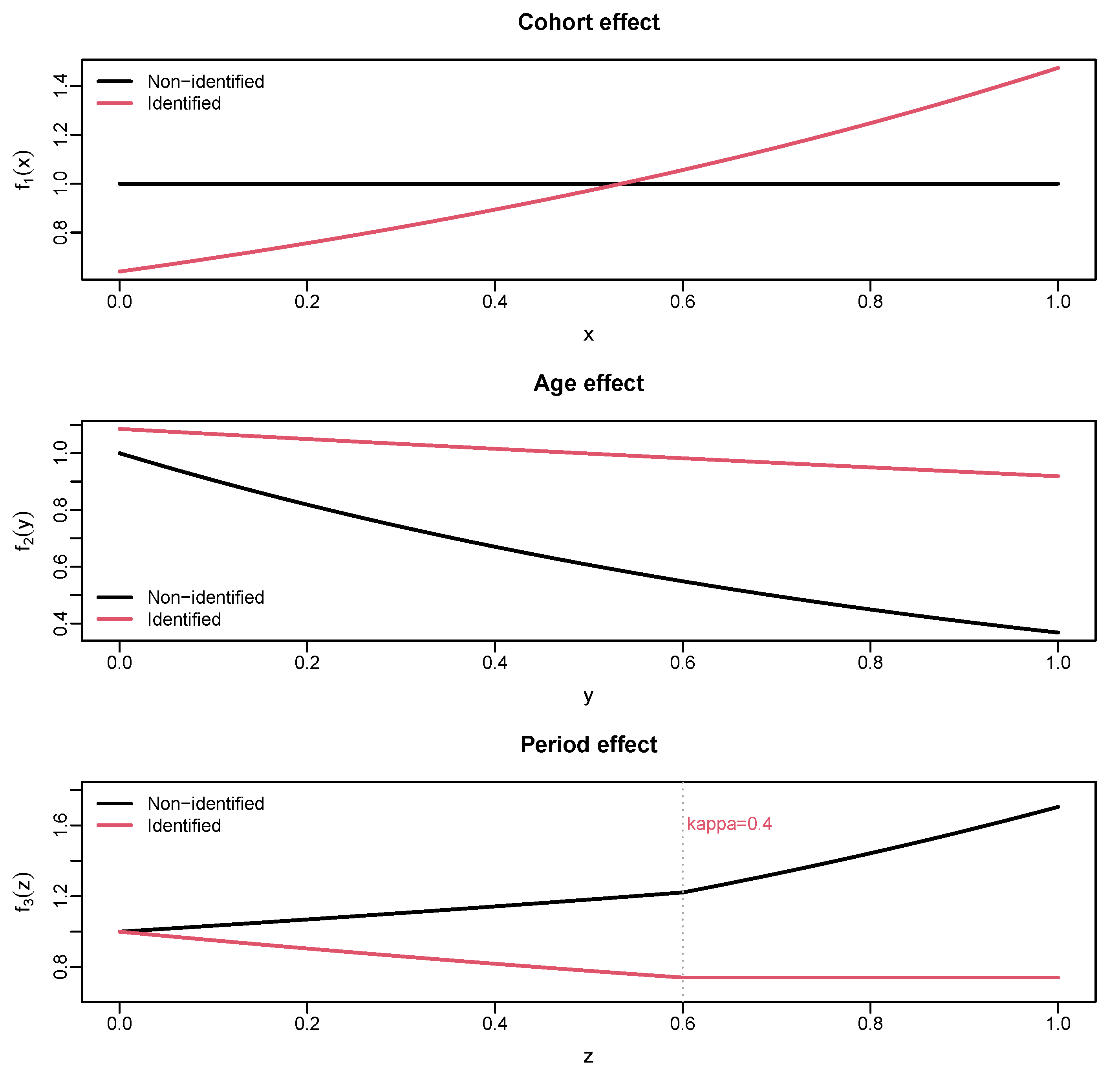
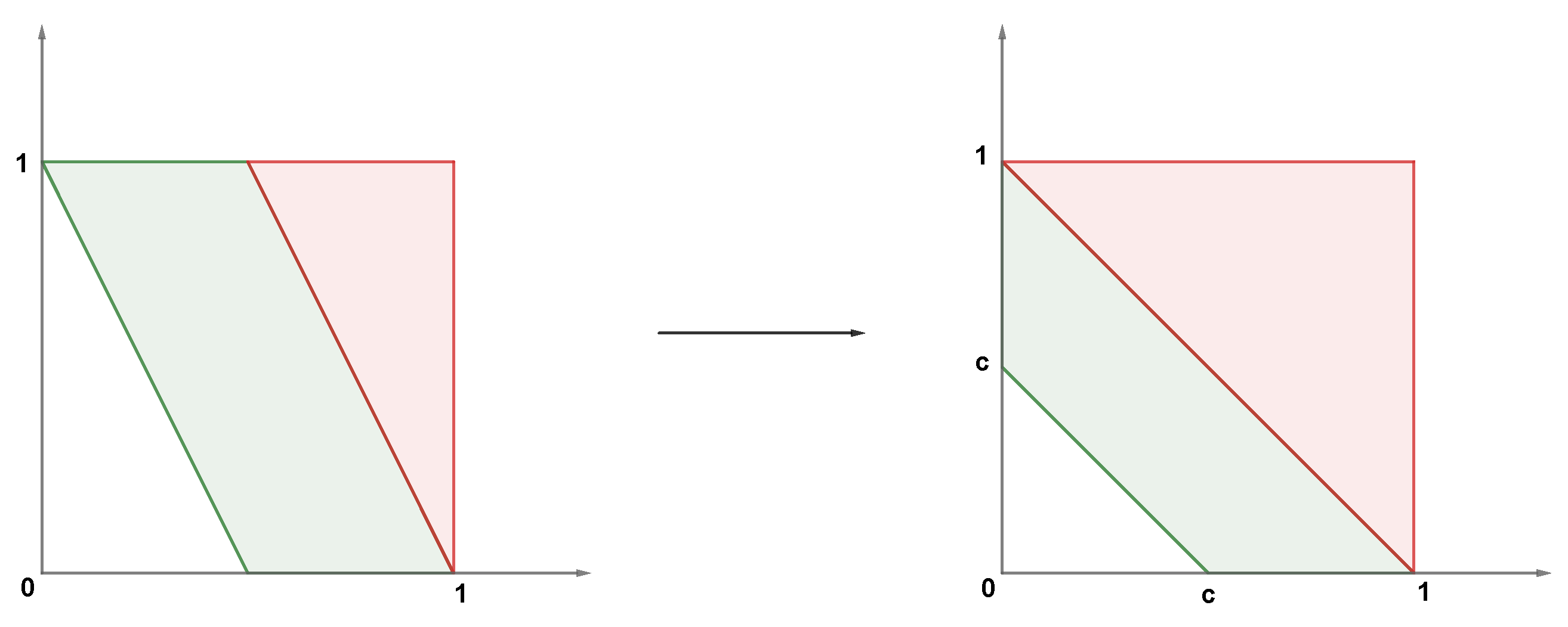
2.1. Density Model
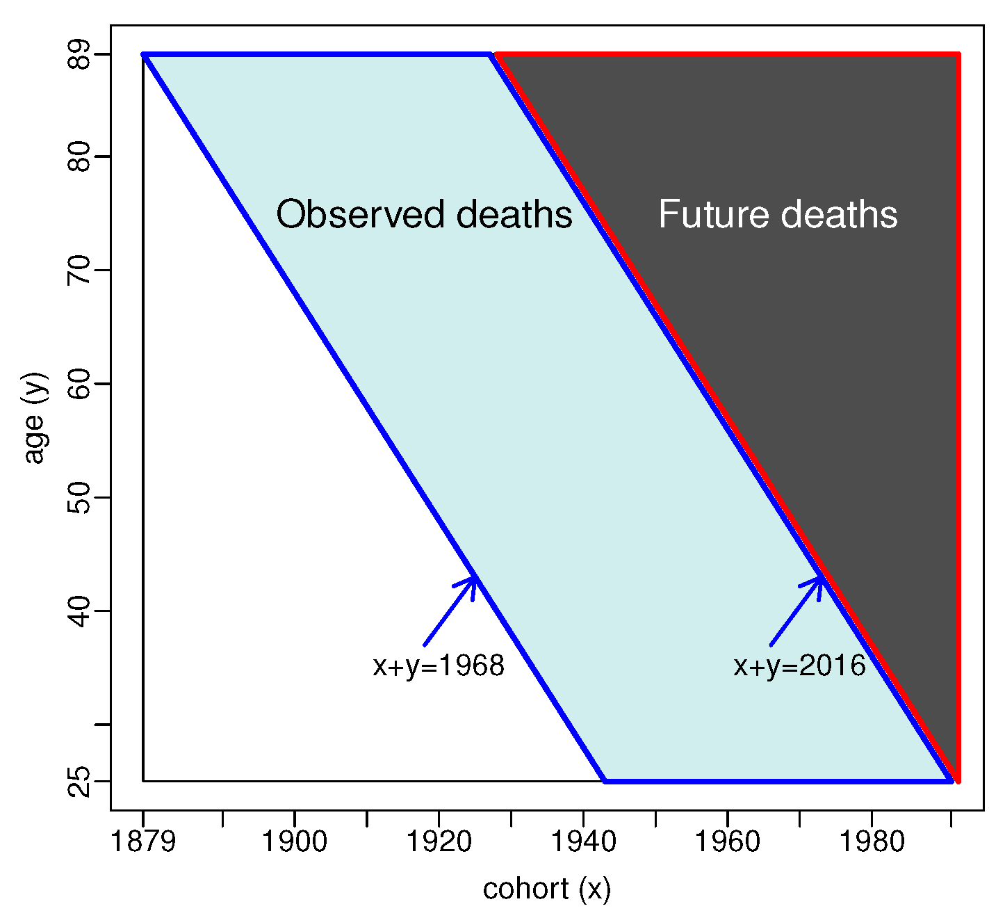
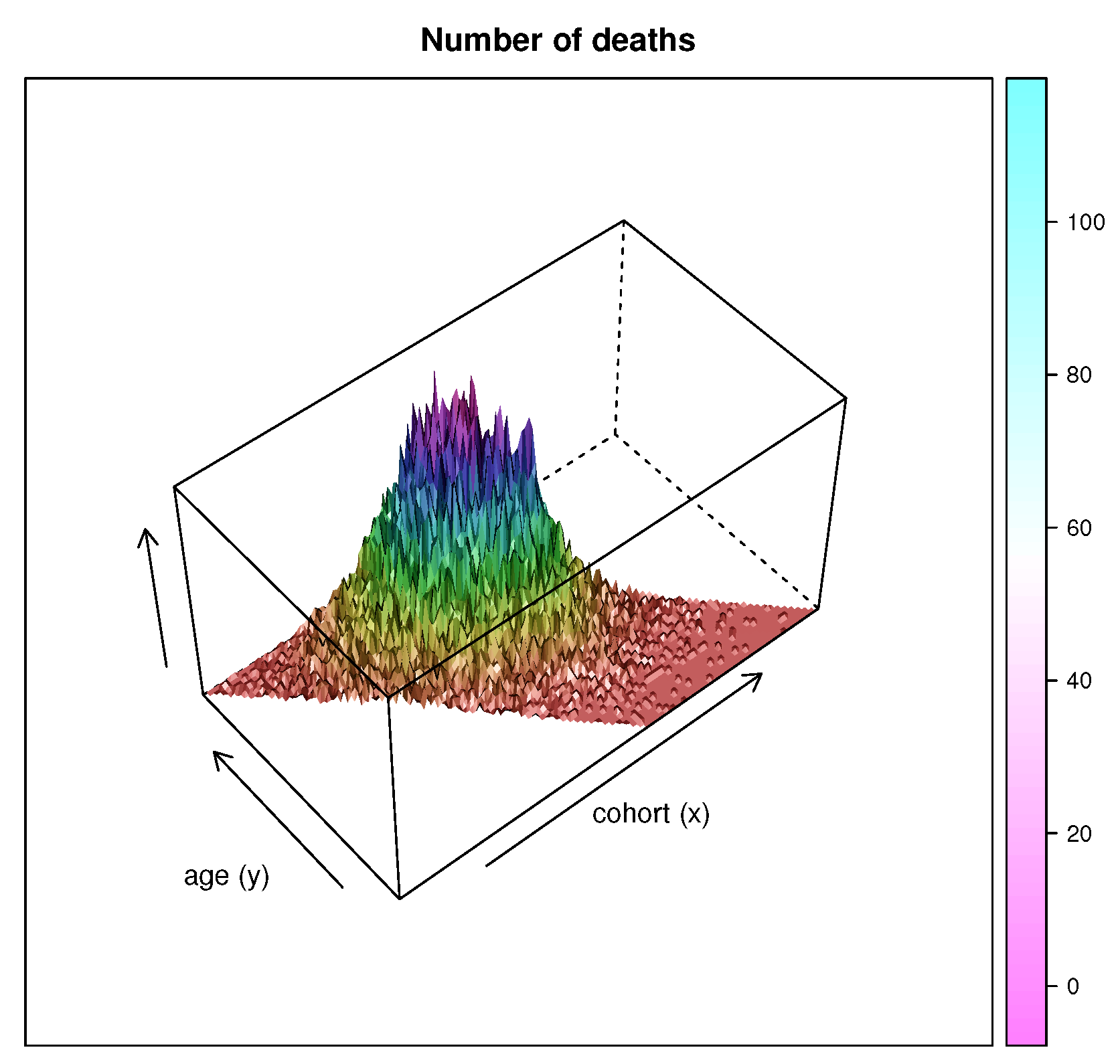
2.2. Data
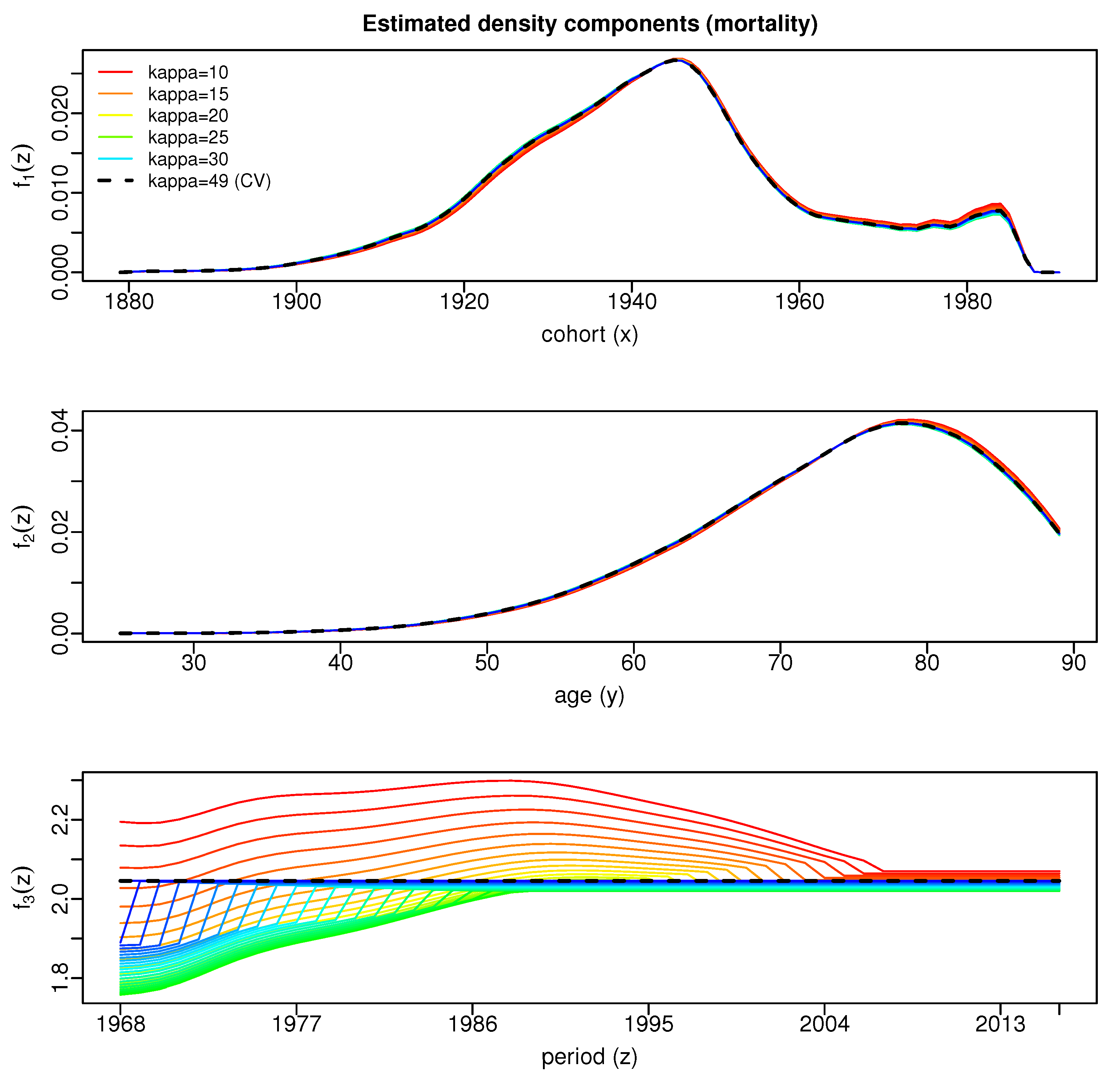
2.3. Estimation
- Step 0.
- Step r.
- Let , and be the backfitting estimates from the previous iteration step. Compute updates as follows.
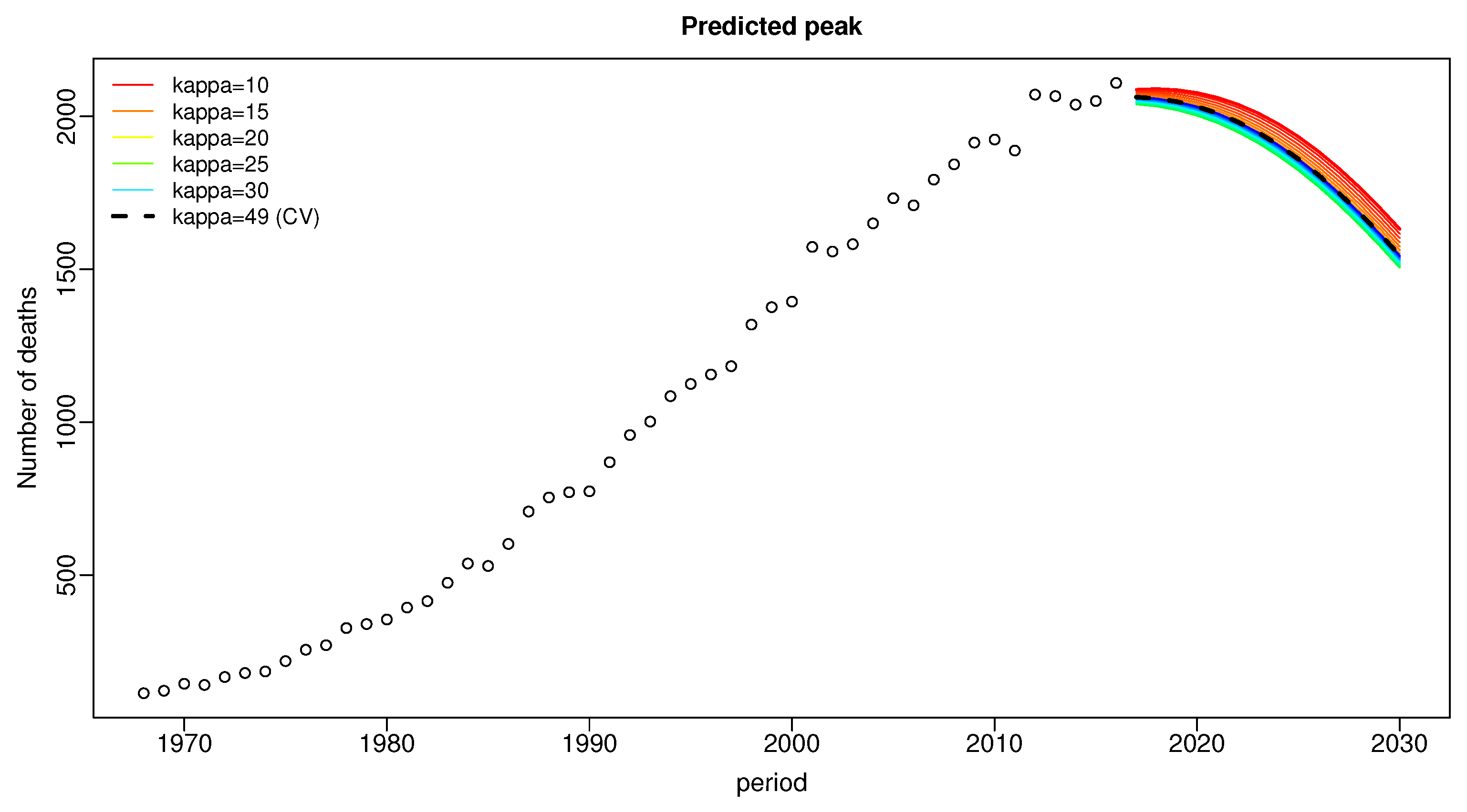
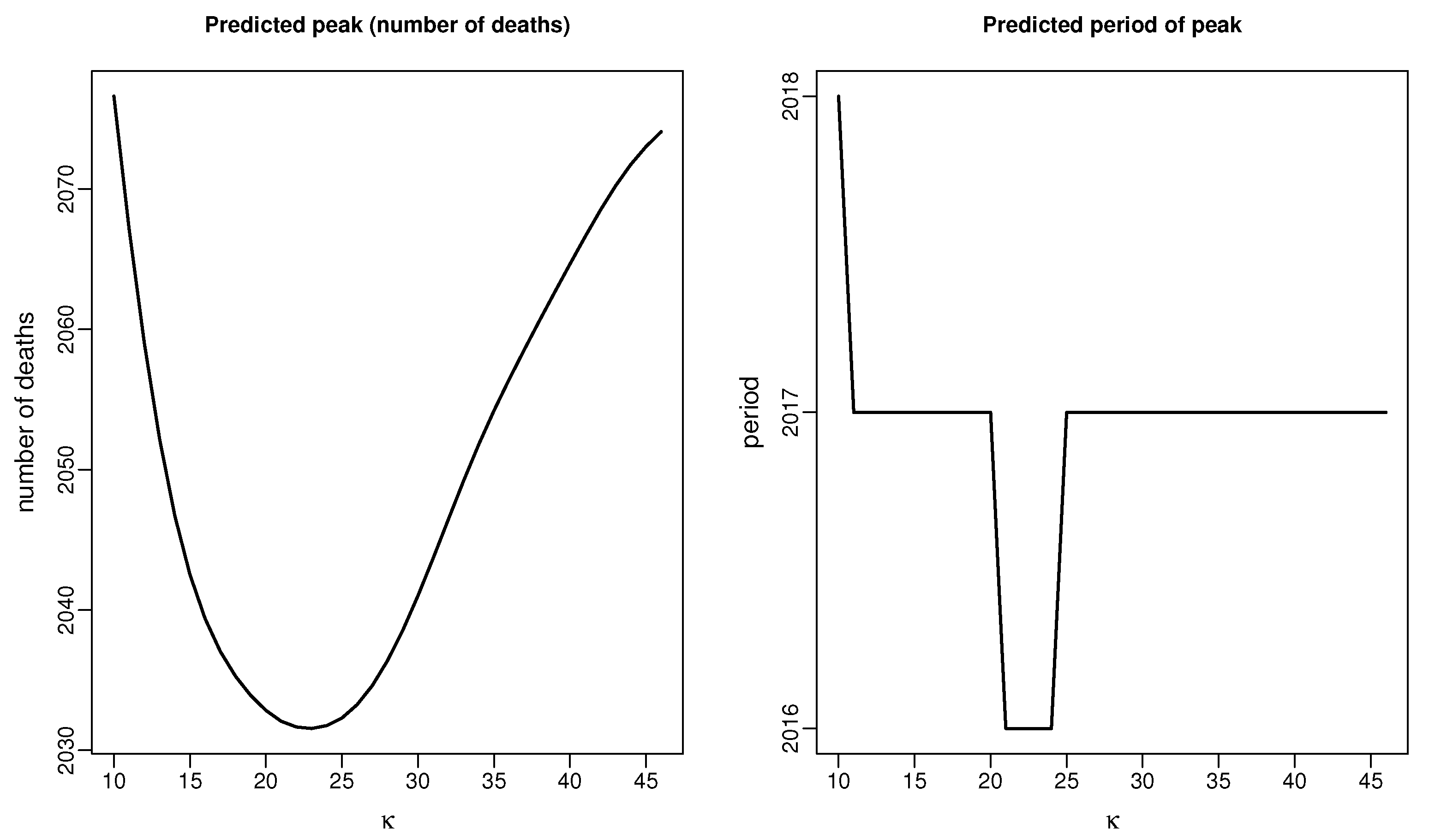
2.4. Forecasting
3. Results
4. Discussion and Conclusions
Author Contributions
Funding
Institutional Review Board Statement
Informed Consent Statement
Data Availability Statement
Acknowledgments
Conflicts of Interest
Appendix A
Appendix B. Two-Dimensional Local Linear Density Estimator
References
- Selby, K. Mesothelioma Statistics. Available online: https://www.asbestos.com/mesothelioma/statistics/ (accessed on 25 August 2021).
- O’Reilly, K.M.; Mclaughlin, A.M.; Beckett, W.S.; Sime, P.J. Asbestos-related lung disease. Am. Fam. Physician 2007, 75, 683–688. [Google Scholar]
- UK Asbestos Working Party. Update from UK Asbestos Working Party. Available online: www.actuaries.org.uk/practice-areas/general-insurance/research-working-parties/uk-asbestos (accessed on 18 December 2020).
- AM Best. Asbestos and Environmental Losses Continue. Available online: http://news.ambest.com/articlecontent.aspx?refnum=281133&altsrc=43 (accessed on 18 December 2020).
- Janssen, F. Advances in mortality forecasting: Introduction. Genus 2018, 74, 21. [Google Scholar] [CrossRef] [Green Version]
- Lee, R.; Carter, L. Modeling and forecasting U.S. mortality. J. Am. Stat. Assoc. 1992, 87, 659–671. [Google Scholar] [CrossRef]
- Hatzopoulos, P.; Haberman, S. A parameterized approach to modeling and forecasting mortality. Insur. Math. Econ. 2009, 44, 103–123. [Google Scholar] [CrossRef]
- Booth, H.; Tickle, L. Mortality modelling and forecasting: A review of methods. Ann. Actuar. Sci. 2008, 3, 3–43. [Google Scholar] [CrossRef]
- Hyndman, R.J.; Ullah, M. Robust forecasting of mortality and fertility rates: A functional data approach. Comput. Stat. Data Anal. 2007, 51, 4942–4956. [Google Scholar] [CrossRef] [Green Version]
- Renshaw, A.; Haberman, S. A cohort-based extension to the Lee-Carter model for mortality reduction factors. Insur. Math. Econ. 2006, 38, 556–570. [Google Scholar] [CrossRef]
- Russolillo, M.; Giordano, G.; Haberman, S. Extending the Lee-Carter model: A three-way decomposition. Scand. Actuar. J. 2011, 2011, 97–117. [Google Scholar] [CrossRef]
- Hodgson, J.; McElvenny, D.; Darnton, A.; Price, M.; Peto, J. The expected burden of mesothelioma mortality in Great Britain from 2002 to 2050. Br. J. Cancer 2005, 92, 587–593. [Google Scholar] [CrossRef]
- Tan, E.; Warren, N. Projection of mesothelioma mortality in Great Britain. In Health and Safety Executive, Research Report; HSE Books: Norwich, UK, 2009; p. 728. [Google Scholar]
- Tan, E.; Warren, N.; Darnton, A.J.; Hodgson, J.T. Projection of mesothelioma mortality in Britain using Bayesian methods. Br. J. Cancer 2010, 103, 430–436. [Google Scholar] [CrossRef] [PubMed]
- Miranda, M.D.M.; Nielsen, B.; Nielsen, J.P. Inference and forecasting in the age–period–cohort model with unknown exposure with an application to mesothelioma mortality. J. R. Stat. Soc. Ser. A Stat. Soc. 2015, 178, 29–55. [Google Scholar] [CrossRef] [Green Version]
- Trotta, A.; Santana, V.S.; Andreozzi, L. P010 Forecasting of Mesothelioma Mortality in Argentina, 2014–2023. Available online: http://dx.doi.org/10.1136/oemed-2016-103951.335 (accessed on 24 August 2021).
- Oddone, E.; Bollon, J.; Nava, C.R.; Consonni, D.; Marinaccio, A.; Magnani, C.; Gasparrini, A.; Barone-Adesi, F. Effect of Asbestos Consumption on Malignant Pleural Mesothelioma in Italy: Forecasts of Mortality up to 2040. Cancers 2021, 13, 3338. [Google Scholar] [CrossRef]
- Algranti, E.; Saito, C.A.; Carneiro, A.P.S.; Moreira, B.; Mendonça, E.M.C.; Bussacos, M.A. The next mesothelioma wave: Mortality trends and forecast to 2030 in Brazil. Cancer Epidemiol. 2015, 39, 687–692. [Google Scholar] [CrossRef]
- Martínez-Miranda, M.D.; Nielsen, B.; Nielsen, J.P. Simple benchmark for mesothelioma projection for Great Britain. Occup. Environ. Med. 2016, 73, 561–563. [Google Scholar] [CrossRef] [PubMed] [Green Version]
- Zehnwirth, B. Probabilistic Development Factor Models with Applications to Loss Reserve Variability, Prediction Intervals and Risk Based Capital; Casualty Actuarial Society Forum: Arlington, VA, USA, 1994; Volume 2, pp. 447–606. [Google Scholar]
- England, P.D.; Verrall, R.J. Stochastic claims reserving in general insurance. Br. Actuar. J. 2002, 8, 443–518. [Google Scholar] [CrossRef]
- Kuang, D.; Nielsen, B.; Nielsen, J.P. Identification of the age-period-cohort model and the extended chain-ladder model. Biometrika 2008, 95, 979–986. [Google Scholar] [CrossRef]
- O’Brien, R. Age-Period-Cohort Models: Approaches and Analyses with Aggregate Data; Chapman and Hall CRC Press: Boca Raton, FL, USA, 2014. [Google Scholar]
- Smith, T.R.; Wakefield, J. A review and comparison of age-period-cohort models for cancer incidence. Stat. Sci. 2016, 31, 591–610. [Google Scholar] [CrossRef]
- Carstensen, B. Age–period–cohort models for the Lexis diagram. Stat. Med. 2007, 26, 3018–3045. [Google Scholar] [CrossRef]
- Clayton, D.; Schifflers, E. Models for temporal variation in cancer rates. I: Age–period and age–cohort models. Stat. Med. 1987, 6, 449–467. [Google Scholar] [CrossRef]
- Clayton, D.; Schifflers, E. Models for temporal variation in cancer rates. II: Age–period–cohort models. Stat. Med. 1987, 6, 469–481. [Google Scholar] [CrossRef] [PubMed]
- Keiding, N. Statistical inference in the Lexis diagram. Philos. Trans. R. Soc. Lond. Ser. Phys. Eng. Sci. 1990, 332, 487–509. [Google Scholar]
- Beutner, E.A.; Reese, S.; Urbain, J.P. Identificability issues of age-period and age-period-cohort models of the Lee-Carter type. Insur. Math. Econ. 2017, 75, 117–125. [Google Scholar] [CrossRef] [Green Version]
- Nielsen, B.; Nielsen, J.P. Identification and forecasting in mortality models. Sci. World J. 2014, 2014, 347043. [Google Scholar] [CrossRef] [PubMed] [Green Version]
- Berzuini, C.; Clayton, D. Bayesian analysis of survival on multiple time scales. Stat. Med. 1994, 13, 823–838. [Google Scholar] [CrossRef]
- Yang, Y.; Land, K.C. Age–period–cohort analysis of repeated cross-section surveys: Fixed or random effects? Sociol. Methods Res. 2008, 36, 297–326. [Google Scholar] [CrossRef] [Green Version]
- Kuang, D.; Nielsen, B.; Perch Nielsen, J. Forecasting in an extended chain-ladder-type model. J. Risk Insur. 2011, 78, 345–359. [Google Scholar] [CrossRef] [Green Version]
- Hunt, A.; Blake, D. Identifiability in age/period/cohort mortality models. Ann. Actuar. Sci. 2020, 14, 500–536. [Google Scholar] [CrossRef]
- Lee, Y.; Mammen, E.; Nielsen, J.P.; Park, B. Asymptotics for in-sample density forecasting. Ann. Stat. 2015, 43, 620–651. [Google Scholar] [CrossRef]
- Mammen, E.; Miranda, M.D.M.; Nielsen, J.P. In-sample forecasting applied to reserving and mesothelioma mortality. Insur. Math. Econ. 2015, 61, 76–86. [Google Scholar] [CrossRef] [Green Version]
- Mammen, E.; Martínez-Miranda, M.D.; Nielsen, J.P.; Vogt, M. Calendar effect and in-sample forecasting. Insur. Math. Econ. 2021, 96, 31–52. [Google Scholar] [CrossRef]
- Miranda, M.D.M.; Nielsen, J.P.; Sperlich, S.; Verrall, R. Continuous Chain Ladder: Reformulating and generalizing a classical insurance problem. Expert Syst. Appl. 2013, 40, 5588–5603. [Google Scholar] [CrossRef]
- Health and Safety Executive (HSE). Mesothelioma Statistics for Great Britain. Annual Statistics. 2019. Available online: www.hse.gov.uk/statistics/ (accessed on 14 July 2021).
- Neilsen, J.P. Multivariate boundary kernels from local linear estimation. Scand. Actuar. J. 1999, 1999, 93–95. [Google Scholar] [CrossRef]
- Mohammadi, B.; Shole Haghighi, A.A.; Khorshidi, M.; De la Sen, M.; Parvaneh, V. Existence of Solutions for a System of Integral Equations Using a Generalization of Darbo’s Fixed Point Theorem. Mathematics 2020, 8, 492. [Google Scholar] [CrossRef] [Green Version]
- Nielsen, B. apc: Age-Period-Cohort Analysis, R Package Version 1.4. Available online: https://cran.r-project.org/web/packages/apc/index.html (accessed on 14 July 2021).
- Wand, M.; Jones, M. Kernel Smoothing; Chapman and Hall: London, UK, 1995. [Google Scholar]


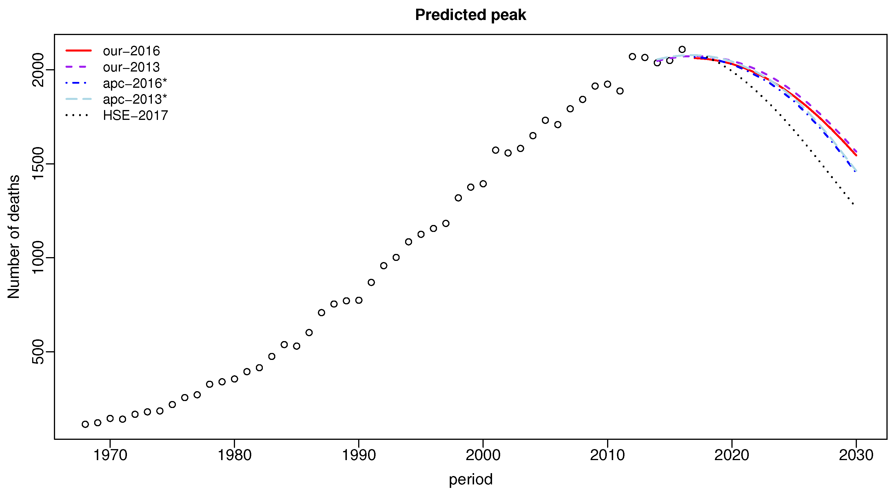
| Period | Data | Our-2016 | apc-2016* | HSE-2017p | Our-2013 | apc-2013* |
|---|---|---|---|---|---|---|
| 2014 | 2032 | 2048 | 2056 | |||
| 2015 | 2042 | 2062 | 2070 | |||
| 2016 | 2101 | 2071 | 2077 | |||
| 2017 | 2087 | 2063 | 2069 | 2074 | 2079 | |
| 2018 | 2058 | 2062 | 2068 | 2072 | 2074 | |
| 2019 | 2048 | 2049 | 2036 | 2063 | 2063 | |
| 2020 | 2032 | 2030 | 1994 | 2049 | 2045 | |
| 2021 | 2010 | 2002 | 1943 | 2028 | 2018 | |
| 2022 | 1982 | 1969 | 1885 | 2002 | 1988 |
Publisher’s Note: MDPI stays neutral with regard to jurisdictional claims in published maps and institutional affiliations. |
© 2021 by the authors. Licensee MDPI, Basel, Switzerland. This article is an open access article distributed under the terms and conditions of the Creative Commons Attribution (CC BY) license (https://creativecommons.org/licenses/by/4.0/).
Share and Cite
Isakson, A.; Krummaker, S.; Martínez-Miranda, M.D.; Rickayzen, B. Calendar Effect and In-Sample Forecasting Applied to Mesothelioma Mortality Data. Mathematics 2021, 9, 2260. https://doi.org/10.3390/math9182260
Isakson A, Krummaker S, Martínez-Miranda MD, Rickayzen B. Calendar Effect and In-Sample Forecasting Applied to Mesothelioma Mortality Data. Mathematics. 2021; 9(18):2260. https://doi.org/10.3390/math9182260
Chicago/Turabian StyleIsakson, Alex, Simone Krummaker, María Dolores Martínez-Miranda, and Ben Rickayzen. 2021. "Calendar Effect and In-Sample Forecasting Applied to Mesothelioma Mortality Data" Mathematics 9, no. 18: 2260. https://doi.org/10.3390/math9182260
APA StyleIsakson, A., Krummaker, S., Martínez-Miranda, M. D., & Rickayzen, B. (2021). Calendar Effect and In-Sample Forecasting Applied to Mesothelioma Mortality Data. Mathematics, 9(18), 2260. https://doi.org/10.3390/math9182260