An Area Coverage Scheme Based on Fuzzy Logic and Shuffled Frog-Leaping Algorithm (SFLA) in Heterogeneous Wireless Sensor Networks

Abstract

Coverage is a fundamental issue in wireless sensor networks (WSNs). It plays a important role in network efficiency and performance. When sensor nodes are randomly scattered in the network environment, an ON/OFF scheduling mechanism can be designed for these nodes to ensure network coverage and increase the network lifetime. In this paper, we propose an appropriate and optimal area coverage method. The proposed area coverage scheme includes four phases: (1) Calculating the overlap between the sensing ranges of sensor nodes in the network. In this phase, we present a novel, distributed, and efficient method based on the digital matrix so that each sensor node can estimate the overlap between its sensing range and other neighboring nodes. (2) Designing a fuzzy scheduling mechanism. In this phase, an ON/OFF scheduling mechanism is designed using fuzzy logic. In this fuzzy system, if a sensor node has a high energy level, a low distance to the base station, and a low overlap between its sensing range and other neighboring nodes, then this node will be in the ON state for more time. (3) Predicting the node replacement time. In this phase, we seek to provide a suitable method to estimate the death time of sensor nodes and prevent possible holes in the network, and thus the data transmission process is not disturbed. (4) Reconstructing and covering the holes created in the network. In this phase, the goal is to find the best replacement strategy of mobile nodes to maximize the coverage rate and minimize the number of mobile sensor nodes used for covering the hole. For this purpose, we apply the shuffled frog-leaping algorithm (SFLA) and propose an appropriate multi-objective fitness function. To evaluate the performance of the proposed scheme, we simulate it using NS2 simulator and compare our scheme with three methods, including CCM-RL, CCA, and PCLA. The simulation results show that our proposed scheme outperformed the other methods in terms of the average number of active sensor nodes, coverage rate, energy consumption, and network lifetime.

1. Introduction

Today, wireless sensor networks (WSNs) have been transformed into an attractive research field for many researchers in industry and academia. These networks include a large number of sensor nodes, which are randomly or deterministically deployed in the network environment without any infrastructure [1,2]. Sensor nodes have been tasked to monitor the Region of Interest (RoI).

WSNs are applied in many applications, such as industry [3], agriculture [3], military [4], medicine [3,5], and Internet of Things (IoT) [4]. Today, micro-electro-mechanical systems have grown dramatically. As a result, many low-cost and robust sensor nodes have been produced [6]. Each sensor node is a multi-functional device including a sensing unit, processing unit, memory unit, communication unit, energy unit, and so on [7,8]. They can sense a target or phenomenon that occurs in their sensing range, they then process the data received from the environment, and finally forward their data packets to the base station (BS) in a single-hop or multi-hop manner [9,10].

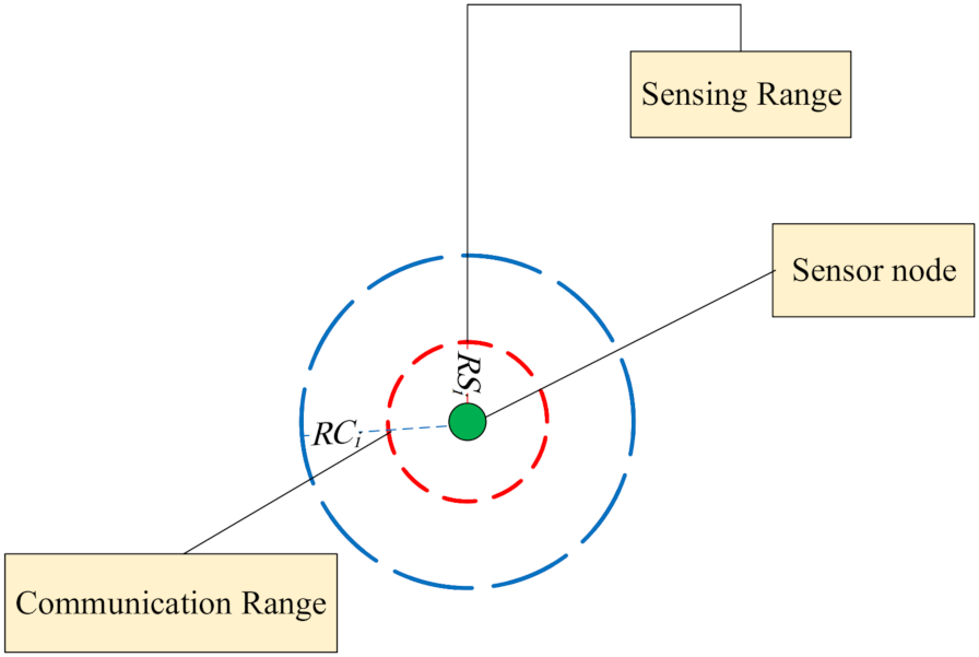
Sensor nodes have small sensing and communication ranges. Furthermore, they have limited energy resources [11,12]. In WSNs, quality of service (QoS) and resource management are two critical issues that must be addressed. QoS is measured based on connectivity and coverage [13,14]. Thus, appropriate coverage and maintenance of connectivity play a important role in the network performance.

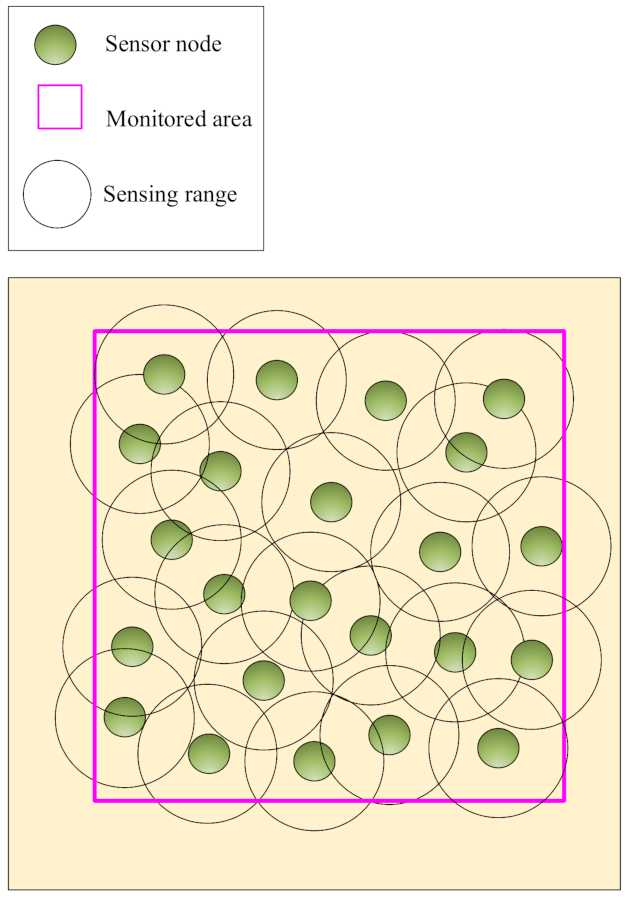
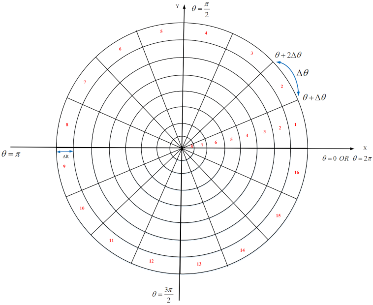
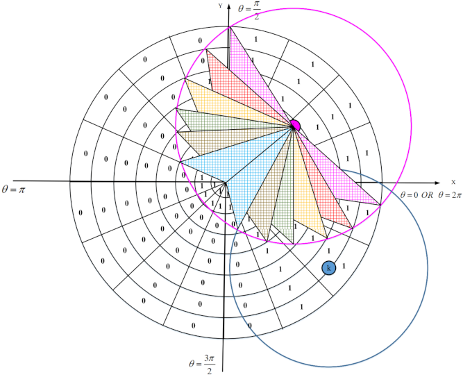
Coverage is defined as the area/point covered or monitored by the sensor nodes deployed in the network area. If an area/point is inside the sensing range of at least one active sensor node; then, it can be said that this area/point have been covered or monitored [15,16]. In general, coverage is classified into several groups according to what exactly is monitored:

• Area coverage: In this coverage, the main goal is to cover or monitor the RoI so that any point in this area should be covered [17,18]. See this coverage type in Figure 1. Area coverage is divided into two categories based on the desired application, including partial and full coverage:
  Partial coverage
  In this coverage, the area is partially covered to guarantee the efficient and acceptable coverage degree according to the desired application. In partial coverage, the goal is to cover the P percentage of the area. This coverage type is also called P-coverage. Partial coverage can save energy of sensor nodes and increase network lifetime. Moreover, it requires a less number of sensor nodes compared to the full coverage [18]. For example, it is sufficient to achieve 80% area coverage in applications, such as environment monitoring, calculating the environment temperature, and forest fire detection during rainy seasons.
  Full coverage
  When it is necessary to cover the entire area, the full coverage is applied. In the full coverage, any point of RoI should be monitored by at least one sensor node. Full area coverage is very costly because it requires a large number of sensor nodes [19]. In addition, the coverage degree is defined based on the application requirements. In some applications, simple coverage is required, i.e., one sensor node is sufficient to cover each point of RoI. However, in other applications, at least k sensor nodes ($k>1$) must cover any point of RoI. In this case, the network is fault-tolerant, and, if a sensor node dies, then the network will continue its normal performance with the $k-1$ sensor nodes; however, this is impossible in simple coverage.
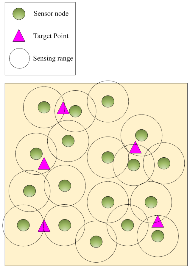
• Point coverage: In this coverage, it is sufficient to monitor some points of RoI depending on the application. It has a low-cost network deployment because fewer sensor nodes are used to cover the target points [20,21]. Figure 2 shows the point coverage.
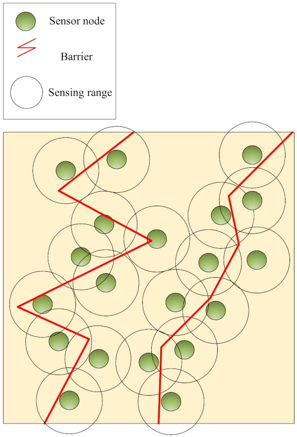
• Barrier coverage: In this coverage, the purpose is to create a barrier using sensor nodes deployed in the network. When sensor nodes sense some subversive activities of attackers at this barrier, they transmit their sensed data to the base station. Barrier coverage is applied in some applications, such as creating infrastructure margins or monitoring important areas, such as country borders, coastlines, battlefield boundaries, and so on [18]. This coverage is shown in Figure 3.
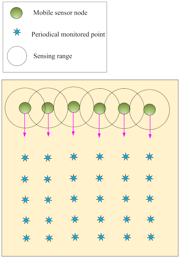
• Sweep coverage: In this coverage, some points of RoI must be monitored periodically, i.e., target points are covered at a certain time interval. Therefore, it is better to cover the target points using a minimum number of mobile sensor nodes [19,22]. Sweep coverage should not be done using static sensor nodes because they have weak performance and additional overhead. This coverage is illustrated in Figure 4.

On the other hand, coverage methods are classified into two categories: centralized coverage schemes and distributed (decentralized) coverage schemes. In centralized coverage methods, only the base station is tasked to manage the coverage process in the network. Whereas, in distributed coverage methods, sensor nodes also participate in this process. In large-scale WSNs, distributed coverage schemes are more efficient because they do not require global information of all sensor nodes in the network, and each sensor node manages the coverage process based on local information received from its neighboring nodes. Coverage methods can be categorized into static and dynamic classes.

In static coverage schemes, the best replacement strategy of sensor nodes is first determined in the network so that proper coverage rate is ensured. Then, this strategy is fixed throughout the network lifetime. However, in dynamic coverage methods, this strategy is always not fixed and updated periodically or when an event occurs [23]. Dynamic coverage methods are more suitable for WSNs due to their limited resources, failure of sensor nodes, and establishing holes.

In most engineering and science problems, it is important to find the maximum or minimum value of a function with different variables. In some cases, there are algorithms based on applied analysis, such as linear programming, that can be used to find the global optimum solution. However, in hybrid or discrete optimization problems, there is no efficient algorithm to find the optimum solution. In the real world, optimization problems are very complex, high dimensions, and highly dynamic.

As a result, it is necessary to use heuristic or metaheuristic methods as algorithms, such as dynamic programming or divide and conquer, have a lot of computational overhead. Today, the metaheuristic algorithms are dramatically becoming popular because they can find acceptable solutions for NP-Hard and nonlinear optimization problems. Metaheuristic algorithms provide a general framework for solving complex optimization problems [24].

These methods are generally inspired by a natural phenomenon. Today, many biological algorithms have been invented or improved. They have successfully been used to solve hybrid and numerical optimization problems—for example, ant colony optimization (ACO) [25], particle swarm optimization (PSO) [26], artificial bee colony (ABC) algorithm [27], shuffled frog-leaping algorithm (SFLA) [28], and artificial immune system (AIS) [29].

Many studies have been presented to solve the coverage problem in WSNs. Coverage techniques focus on several issues: designing a replacement strategy for sensor nodes in the network environment, designing a scheduling mechanism for sensor nodes, and selecting a subset of nodes for full coverage. We review a number of papers related to the research subject in Section 2 and express their strengths and weaknesses.

Most of these methods do not consider the energy of the sensor nodes in the network. They have a lot of communication overhead, which threatens the network lifetime. Moreover, they are often centralized and static schemes and propose no useful strategy for reconstructing holes created in the network. These problems reduce their scalability and network lifetime. Therefore, it is necessary to design an efficient area coverage method, which schedules the activity of sensor nodes in the network intelligently.

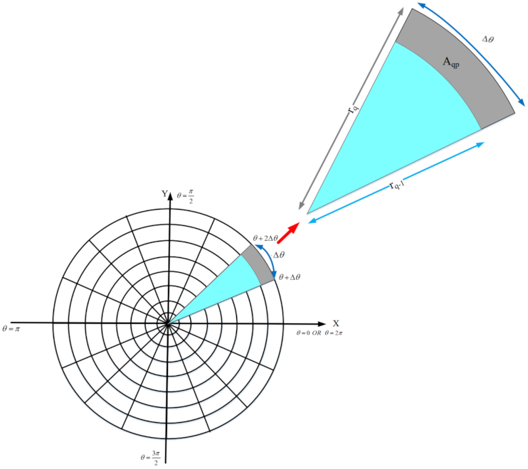
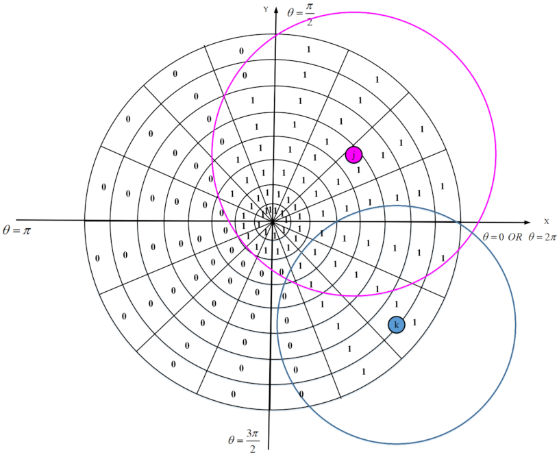
We design an appropriate strategy for reconstructing holes in the network. Furthermore, it is important and critical to calculate the overlap of nodes to select the lowest number of active sensor nodes in the network. However, calculating the overlap between the sensing ranges of sensor nodes is a complicated, time-consuming, and difficult task due to limited resources and low energy of sensor nodes.

In this paper, we present a simple, efficient, and distributed method to calculate the overlap between sensor nodes. The purpose of this paper is to present a suitable area coverage scheme for heterogeneous WSNs, and thus this method can balance the energy consumption of sensor nodes in the network and improve network lifetime. We attempt to increase the coverage quality in the network. The main contributions of the paper are expressed as follows:

• In the first phase, each sensor node estimates the overlap between its sensing range and sensing ranges of neighboring nodes using a distributed method based on geometric mathematics. Calculating the overlap between the sensing range of a sensor node and its neighboring nodes is a complex operation with a lot of computational overhead and high time complexity. In the proposed method, we attempt to reduce computational overhead and introduce a new, efficient and distributed method based on a digital matrix to calculate the overlap.
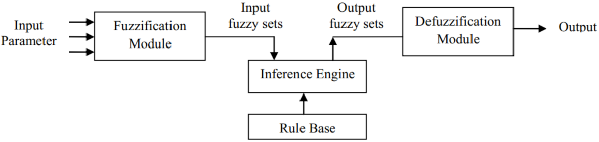
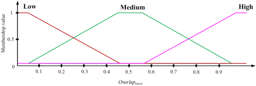
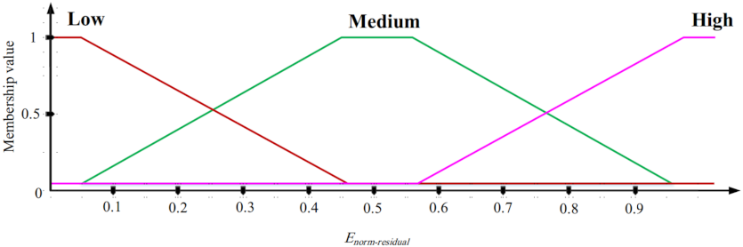
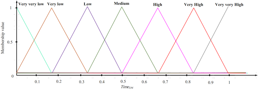
• In the second phase, the goal is to design an ON/OFF scheduling mechanism based on fuzzy logic. This fuzzy system has three inputs: the overlap between sensing range of a sensor node and sensing ranges of its neighboring nodes, the residual energy, and the distance between a sensor node and BS. The fuzzy system output is the activity time of each sensor node (ON time). In this fuzzy system, if the overlap between the sensing range of a sensor node and sensing ranges of neighboring nodes is low and its energy level is high and the distance between this node and BS is low, then this node stays at the ON state for more time slots.
• In the third phase, we attempt to present a suitable method that predicts the death time of sensor nodes and prevents possible holes in the network, and thus there is no interruption in the data transmission process to the base station.
• In the fourth phase, the goal is to find the best replacement strategy for mobile nodes to maximize the coverage rate and minimize the number of mobile nodes applied for covering holes. For this purpose, we use the shuffled frog-leaping algorithm (SFLA) and present a suitable and multi-objective fitness function.

The rest of paper is organized as follows: In Section 2, some recent studies are reviewed in the coverage field for WSNs. In Section 3, the basic concepts used in the proposed scheme, namely the fuzzy logic and the shuffled frog-leaping algorithm (SFLA), are described briefly. In Section 4, we present the system model in the proposed method. This model includes the network model, energy model, sensing model, and communication model. In Section 5, we define the problem studied in this paper. In Section 6, the proposed scheme is described in detail. In Section 7, the simulation results of the proposed scheme are presented and compared with some coverage methods. Finally, our conclusions are presented in Section 8.

2. Related Works

Coverage is one of the most important and fundamental issues in WSNs, because it has a direct effect on the energy consumption of sensor nodes and network lifetime. Generally, coverage is defined as monitoring on the network environment effectively and efficiently. Today, many papers have been published in the coverage field in WSNs. These papers often focus on three concepts: deploying sensor nodes in a predetermined manner, designing a scheduling mechanism, and selecting a subset of sensor nodes for ensuring full coverage. In the following, we briefly introduce some coverage methods.

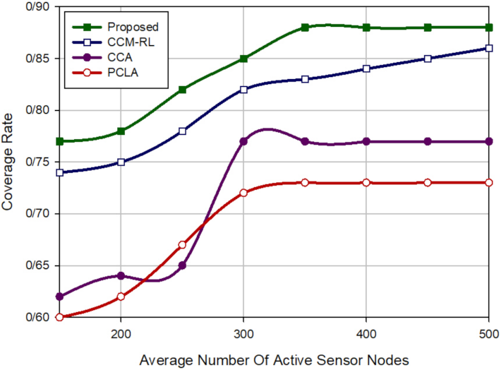
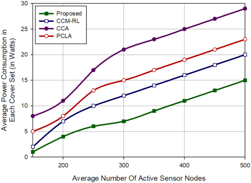
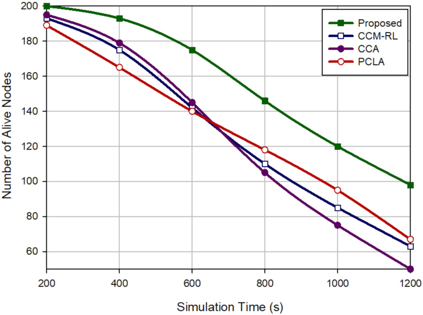
Sharma et al. [30] suggested the coverage connectivity maintenance based on reinforcement learning (CCM-RL) protocol in wireless sensor networks. The purpose of this method is to achieve the maximum coverage rate, maintain connectivity, and save energy efficiently. In this scheme, the learning algorithm is implemented in each sensor node. This algorithm allows them to automatically learn their optimal activity. The purpose of this algorithm is that only subsets of sensor nodes are activated in each scheduling round to minimize energy consumption, maximize the coverage rate, and maintain network connectivity.

In addition, CCM-RL presents a sensing range customization mechanism for removing coverage redundancy. After executing the learning algorithm, active sensor nodes, which overlap with each other, should customize their sensing range using this mechanism to maintain network resources, such as energy and memory, reduce duplicated data packets, and lower network congestion. CCM-RL is a dynamic and distributed coverage method, that is, the sensor nodes participate in the scheduling process.

As a result, CCM-RL is a scalable scheme. However, CCM-RL schedules sensor nodes based on only two parameters, including distance and coverage rate. It ignores energy parameters in this process. Furthermore, CCM-RL may have a lot of delay. This method does not provide any mechanism for detecting or reconstructing coverage holes in the network.

Yu et al. [31] presented two centralized and distributed protocols based on the coverage contribution area (CCA) concept to solve the K-coverage problem in homogeneous wireless sensor networks. The purpose of this method is to achieve K-coverage with a minimum number of sensor nodes and improve network lifetime. CCA presents a scheduling process to activate a subset of sensor nodes for covering the RoI. This process is based on two criteria, including energy and distance. After implementing this algorithm, nodes are in two modes, including ON (active) or OFF (inactive).

Yu et al. introduced the centralized k-coverage protocol in two dynamic and static modes. However, the dynamic scheme has a higher delay than the static method; but it provides better coverage. In general, the centralized CCA is not scalable. As a result, it is not suitable for the large scale WSN. As the sink node requires global information of all sensor nodes in the network. The distributed CCA is scalable and solves the problem of the centralized CCA method, but it has high communication overhead. CCA presents no detection and reconstruction mechanism for repairing network holes.

Mostafaei et al. [32] offered a partial coverage with learning automata (PCLA) scheme in WSNs. The main purpose of this method is to minimize the number of sensor nodes required for covering RoI and maintain connectivity. PCLA uses the learning automata (LA) for scheduling sensor nodes. This scheme provides a probabilistic framework to select the subset of the sensor nodes to create a backbone to improve the coverage rate and guarantee network connectivity.

PCLA has two phases: (1) The learning phase. In this phase, subsets of sensor nodes are selected to create a backbone in the network so that network connectivity is guaranteed. (2) The partial coverage phase. If the selected subset in the first phase cannot provide a suitable coverage rate of the RoI, additional nodes are added to this subset to satisfy the appropriate coverage level. PCLA is a distributed, dynamic and scalable method. However, it has a lot of communication overhead. Moreover, PCLA does not present any mechanism for detecting and reconstructing network holes.

Hanh et al. [33] proposed an area coverage method based on genetic algorithm (GA) called MIGA in heterogeneous WSNs. MIGA is an improved version of IGA. In this method, a stable and reliable fitness function was presented to evaluate the area coverage approximately.

MIGA has five phases: (1) Individual representation. In this phase, each genotype is divided into k sections corresponding to k sensor types and each section has several genes. (2) Population initialization. In this phase, population initialization is not random. In fact, it is done based on a heuristic algorithm. (3) Genetic operators. In MIGA, two crossover operators are used, namely Laplace crossover (LX) and Arithmetic crossover method (AMXO). Then, generated individuals are sorted based on location of sensor nodes in the network. (4) Designing the fitness function. In MIGA, an integral-based fitness function has been proposed to evaluate the RoI coverage. (5) VFA Optimization.

When the MIGA algorithm is stopped, the best solution can be improved using Virtual Force Algorithm (VFA) to maximize area coverage. In this phase, the overlapping sensor nodes are slightly spaced apart to reduce their overlap. As a result, each sensor node executes a local search with neighboring nodes to optimize the final solution. MIGA has several advantages: achieving a stable and quality solution and maximizing area coverage.

Furthermore, this method has certain disadvantages: (1) The integral-based fitness function is not comprehensive and cannot cover all different cases that two sensor nodes may overlap with each other. However, this method introduce a new idea for calculating the overlap between different sensor nodes and can be improved. (2) In this MIGA, the authors attempted to reduce the computational overhead, but they achieved little success. (3) In this method, a centralized area coverage scheme was presented. Therefore, it was not scalable.

Luo et al. [34] introduced the maximum coverage sets scheduling (MCSS) problem in WSNs. The purpose of this scheme is to find the optimal scheduling strategy for coverage sets to maximize the network lifetime. In this method, two algorithms, called greedy-MCSS and MCSSA, were presented to solve this problem. This method has the advantages: (1) acceptable time complexity, (2) appropriate computational complexity, and (3) improving the network lifetime through the proper scheduling of coverage sets.

However, this method also has disadvantages: (1) It is assumed that the coverage sets are predetermined (the coverage set represents a subset of sensor nodes in the network that can cover the entire network). However, it is important to define these sets. However, the authors ignored this problem. (2) Furthermore, it is assumed that the time slots required for the activity of sensor nodes are already known, whereas this is a false hypothesis that can limit the application of this method. (3) The MCSSA algorithm is a centralized method. As a result, it is not scalable and cannot be desirable for large-scale WSNs. (4) The authors only considered the activity time of the sensor nodes for solving the MCSS problem. However, this is an important weakness because other parameters, such as the energy and distance of nodes from each other, are critical.

Benahmed et al. [35] presented an optimal barrier coverage method that minimizes the number of sensor nodes and maximizes the coverage rate in homogeneous WSNs. This method can calculate the minimum number of sensor nodes that cover a 2D area completely. Moreover, a geometric mathematics-based formula was proposed for calculating the coverage value. In this method, the minimum number of sensor nodes was calculated based on the distance and angle between two neighboring nodes that have overlap.

In addition, the authors presented an algorithm to reduce overlap between sensor nodes as much as possible so that appropriate distance between two sensor nodes is obtained based on the optimal number of nodes and the maximum coverage rate. They proposed a mechanism for detecting failed nodes and reconstructing holes created in the network. The most important advantage of this method is the appropriate coverage rate with the minimum number of sensor nodes.

On the other hand, the geometric mathematical model presented in this method is a novel and attractive solution that can be improved. This method takes into account parameters, like the distance and the overlap between the sensor nodes, to determine the coverage rate of the network. This method can be improved by considering more parameters, such as the energy of the sensor nodes.

One of the disadvantages of this scheme is that it applied a reactive mechanism for detecting failed nodes and reconstructing holes in the network, i.e., when a failed node or hole is identified, then this mechanism is executed to repair it. This can disrupt network performance and increase delay in the data transmission process to BS. Therefore, it is better to use predictive methods to detect nodes that may be damaged in the near future.

Saha et al. [36] introduced a suitable and rapid scheme to approximate the area covered in homogeneous WSNs. This approach utilizes digital geometry to approximate a real circle (i.e., sensing range of each sensor node) using a digital circle. The authors argue that their proposed algorithm has less computational complexity and lower time complexity than geometric mathematics-based operations executed on a real circle.

In addition, each digital circle is estimated using two squares: (1) the largest square inside the circle and (2) the smallest square outside the circle. As a result, this method can estimate the area covered by each sensor node with an acceptable error rate and appropriate time complexity. The authors proposed a fast, simple and distributed algorithm, which has low computational overhead, to estimate the total area covered in the network. As a result, it is suitable for energy-limited WSN.

However, the authors added some points to improve the performance of this method: (1) In this method, a suitable scheduling mechanism was not designed to adjust the activity time of nodes. Moreover, it is important to take into account various parameters, such as the node energy for modeling this mechanism. (2) This method ignores a reconstruction and detection mechanism to repair holes created in the network due to the death of some sensor nodes. (3) This method is a static area coverage scheme, whereas, WSNs have a dynamic topology and are more compatible with dynamic schemes.

Binh et al. [37] proposed two nature-based algorithms, including improved cuckoo search (ICS) and chaotic flower pollination algorithm (CFPA), to improve area coverage in heterogeneous WSNs. The purpose of this method is to reduce energy consumption of sensor nodes. This method has several steps, including individual representation, initialization and fitness function, and updating individuals. Refer to [37] for more details.

The proposed fitness function in these algorithms is based on the overlap between sensing range of sensor nodes. Obviously, if the overlap between sensor nodes is reduced, then they can cover a larger area. ICS and CFPA algorithms can reduce computational complexity and generate high quality responses. Another advantage of these algorithms is their simplicity and high convergence speed.

However, these two algorithms also have disadvantages: (1) The fitness function considers only one parameter, namely the overlap between the sensor nodes. However, it can improve with considering more parameters. (2) This method is a static area coverage. It searches for the best replacement strategy for sensor nodes. However, it does not provide a reconstruction and detection mechanism to resolve problems related to death of some sensor nodes and hole establishment in the network.

Binh et al. [38] proposed two meta-heuristic algorithms, namely genetic algorithm (GA) and particle swarm optimization (PSO) to maximize the area coverage in a heterogeneous WSN. It is assumed that network includes a number of obstacles, which block communications between sensor nodes. Therefore, the authors have defined the maximum area coverage problem in a network having obstacles and have proposed two algorithms GA and PSO to solve this problem.

In this method, a novel fitness function was designed based on the overlap between sensing ranges of the sensor nodes with respect to obstacles in the network. The purpose of these algorithms is to reduce the overlap between sensor nodes in the network. Refer to [38] for more details. These algorithms have an important advantage: maximizing the area coverage with acceptable computational overhead.

However, this method also has disadvantages: (1) It considers only one parameter i.e., the overlap for designing fitness function. (2) In this method, the aim is maximum area coverage. However, the maximum network lifetime is also important. If the residual energy of the sensor nodes has been considered in the fitness function, then it can also improve network lifetime. (3) This is a static and centralized area coverage method. Thus, it has low scalability.

Li et al. [39] presented a reasonable mathematical model to solve the weak coverage problem in WSNs. The area coverage algorithm can adjust movement direction of the sensor nodes toward low-density areas, and thus that the area coverage is maximized. As a result, sensor nodes are almost distributed in the network uniformly. The authors improved the virtual force algorithm. Refer to [39] for more details.

This method has several advantages: (1) maximizing the network coverage rate and (2) a low computational complexity. However, this method also has some disadvantages: (1) It is a centralized area coverage method, whereas distributed area coverage schemes are more desirable for WSNs. (2) This method does not take into account the network lifetime. Considering energy of the nodes is important in WSNs. (3) This area coverage method is static. This can weaken its efficiency.

Kashi et al. [40] proposed a heterogeneous distributed precise coverage rate (HDPCR) mechanism, which calculates the area coverage in a distributed manner. This method can detect the network boundaries, holes, and stains using simple mathematical calculations and compute the entire area covered in the network exactly. This process is locally done and each sensor node participates in it. This method includes several important advantages: (1) a low computational overhead and (2) a distributed area coverage method that is more suitable for WSNs than for centralized schemes.

However, it suffers from several major weaknesses: (1) High communication overhead. (2) This method only calculates the area covered in the network. It does not describe the purpose of these operations. Generally, the main purposes of an area coverage method are searching for the best replacement strategy for sensor nodes in the network, obtaining the best area coverage quality with the minimum sensor nodes, achieving the maximum network lifetime, designing suitable scheduling schemes, and so on.

Therefore, calculating the area covered in the network alone is not the main goal of an area coverage method. (3) In this approach, the covered area is locally calculated through the sensor nodes in the network. If one of the sensor nodes performs its calculations incorrectly, then the final result will not be accurate.

Miao et al. [41] introduced a grey wolf optimizer with enhanced hierarchy (GWO-EH) that improved the grey wolf optimizer (GWO) algorithm. The authors claimed that GWO-EH can solve certain weaknesses of GWO, such as the low convergence speed and becoming trapped in local optimum. They solved the convergence rate by improving the weight coefficients. To balance global and local searches, they improve the position updating equation. Then, they applied GWO-EH to solve the area coverage problem in homogeneous WSNs.

The experiments indicate that this method has a suitable convergence rate. However, this method also has some disadvantages: (1) In this scheme, if the number of sensor nodes in the network is increased, then the convergence rate will be reduced. Therefore, this method is not scalable. (2) Its computational complexity is high. (3) This is a centralized area coverage method. (4) It is a static coverage scheme and cannot provide a suitable reconstruction and detection mechanism for covering holes established in the network.

Table 1. Various coverage methods.

Number	Scheme	Purpose	Advantages	Disadvantages
1	[30]	Achieving energy-efficient coverage, and maintaining connectivity	Scalability, designing the dynamic and distributed coverage method, presenting the sensing range customization mechanism, low network congestion, low energy consumption, high coverage rate	High delay, ignoring energy of nodes in the scheduling process, not designing a detection and reconstruction mechanism for covering holes
2	[31]	Solving the K-coverage problem with the minimum sensor nodes	Scalability, appropriate computational overhead, considering energy of nodes in the scheduling process, presenting a dynamic and distributed K-coverage scheme, improving network lifetime	High delay, high communication overhead, not designing a detection and reconstruction mechanism for covering holes
3	[32]	Minimizing the number of sensor nodes required for partial area coverage and network connectivity maintenance	Scalability, presenting a dynamic and distributed coverage scheme, guaranteeing network connectivity, achieving an appropriate coverage level of the RoI	High communication overhead, not designing a detection and reconstruction mechanism for covering holes
4	[33]	Maximizing area coverage	Achieving a high quality and appropriate solution, increasing area coverage	Incomplete fitness function for evaluating area covered, high computational overhead, a centralized area coverage, low scalability
5	[34]	Finding the optimal scheduling strategy for coverage sets and maximizing network lifetime	Acceptable time complexity, appropriate computational complexity, improving network lifetime using a suitable scheduling mechanism	Not designing a mechanism for determining coverage sets, considering predetermined time slots for sensor node activity, presenting a centralized algorithm, low scalability, ignoring parameters, such as the distance between sensor nodes and energy
6	[35]	Designing a barrier coverage method with minimum sensor nodes and maximizing the coverage rate	Achieving a suitable coverage rate with a minimum number of sensor nodes, presenting a novel scheme for calculating coverage rate based on geometric mathematics	Considering insufficient parameters for calculating the coverage rate, designing a reactive detection and reconstruction mechanism for repairing network holes, making interruption and delay in the network performance
7	[36]	Presenting a fast and efficient method for estimating area covered	Appropriate time complexity, acceptable computational complexity, low error rate (high accuracy), introducing a distributed method for estimating the total area covered in the network	Not designing a proper scheduling mechanism, not designing a detection and reconstruction mechanism for covering holes, presenting a static area coverage method
8	[37]	Maximizing area coverage in the network	Appropriate computational complexity, generating high quality solutions, simplicity and appropriate convergence rate	Not considering various parameters in the fitness function, proposing a static area coverage method
9	[38]	Maximizing area coverage in a network with obstacles	Achieving the maximum area coverage rate, appropriate computational overhead	Not considering various parameters in the fitness function, not considering the maximization network lifetime, proposing a static area coverage method, low scalability
10	[39]	Improving area coverage and reducing the distance traveled by mobile nodes	Maximizing coverage rate, very low computational complexity	Presenting a static and centralized area coverage scheme, not considering the node energy for improving the network lifetime
11	[40]	Calculating coverage rate in a distributed manner	Low computational overhead, introducing a distributed area coverage scheme	High communication overhead, not designing a suitable coverage mechanism, high error rate for calculating the coverage rate
12	[41]	Maximizing area coverage	Proper convergence rate, ability for finding optimal solution	Low scalability, high computational complexity, providing a centralized and static area coverage method

lists the advantages and disadvantages of different coverage schemes, which were briefly reviewed in this section.

3. Basic Concepts

In this section, we illustrate some the basic concepts, including fuzzy logic and the shuffled frog-leaping algorithm (SFLA). These concepts have been applied in the proposed scheme.

3.1. Fuzzy Logic

Based on the research studies, it can be deduced that measuring, modeling, and controlling real and complex processes are not accurate because there are uncertainties, such as incompleteness, randomness and data loss. Fuzzy logic (FL) is a mathematical technique [42]. Its aim is to describe approximately human thinking. Unlike classical set theory, in which the outputs are either true or false, fuzzy logic generates partial values based on inference rules and linguistic variables.

Today, fuzzy inference mechanisms are widely applied in various applications. In the following, we refer to some applications. Vilela et al. in [43] combined fuzzy logic with the Value of Information (VoI) assessment system. This scheme has been developed to evaluate the oil and gas subsurface. Nguyen et al. [44] presented the Fuzzy Q-Charging method to determine the optimal amount of energy charging for sensor nodes using fuzzy logic.

Bayrakdar in [45] used the fuzzy logic technique to select the lowest number of sensor nodes for monitoring the agricultural environment. Peng et al. [46] used fuzzy logic to design a transmission power allocation strategy (TPA) to maximize the lifetime of WSN. Baradaran and Navi in [47] proposed the HQCA clustering method, which uses fuzzy logic to choose the cluster head nodes in WSNs. We used fuzzy logic in our paper to design a scheduling mechanism for sensor nodes in the network. Two well-known fuzzy inference mechanisms are Mamdani fuzzy inference and Sugeno fuzzy inference (TSK).

A fuzzy system has four main modules: fuzzification, defuzzification, a fuzzy rule base, and a fuzzy inference engine. A fuzzy system is shown in Figure 5. The fuzzification module maps the system inputs to the fuzzy sets and determines their fuzzy membership degree. These fuzzy values are simulated using an inference engine that uses fuzzy rules stored as IF-THEN rules. The results of the inference system are in the fuzzy form, which are transformed into crisp values using a defuzzification module, such as an averaging scheme and the centroid scheme [42].

Today, fuzzy inference mechanisms are widely applied in various applications. In the following, we refer to some applications. Vilela et al. in [43] combined fuzzy logic with the Value of Information (VoI) assessment system. This scheme has been developed to evaluate the oil and gas subsurface. Nguyen et al. [44] presented the Fuzzy Q-Charging method to determine the optimal amount of energy charging for sensor nodes using fuzzy logic.

3.2. Shuffled Frog-Leaping Algorithm (SFLA)

The shuffled frog-leaping algorithm (SFLA) is a metaheuristic algorithm inspired by the foraging behavior of frogs. Eusuff et al. [28] introduced the SFLA in 2006. This algorithm has two elements, including local search and global information exchange. In SFLA, an initial population of frogs is divided into several groups called memeplexes. In general, there are two search methods: (1) local search, which searches the optimal position in each group, and (2) Global search, in which information is exchanged between different groups.

In the local search process, each memeplex is partitioned into a number of sub-memeplexes. Then, frogs are evaluated based on a fitness function and are sorted in descending order according to their fitness values to determine the best and worst frogs in each the sub-memeplex, which are described as $P_B$ and $P_w$, respectively. Then, the position of the worst frog ($P_w$) is improved toward the best frog ($P_B$) using Equation (1):

$$U\left(q\right)=P_w+S_i$$

(1)

where $U\left(q\right)$ is the new position frog, $S_i$ indicates the step size, and thus $S_{min}\le S_i\le S_{max}$.

$$S_i=Rand\times \left(P_B-P_w\right)$$

(2)

where $Rand$ is a random number in $\left[0,1\right]$. If the fitness value of the new position is better than the old position, then the new position is replaced with the old position. Otherwise, the new position is removed, and a new position is calculated based on Equation (3):

$$S_i=Rand\times \left(P_X-P_w\right)$$

(3)

where $P_X$ represents the best position in the memeplex. If the new position is better than the old position, then it is replaced with the old position. Otherwise, the new position is deleted. Then, a new solution is randomly calculated according to Equation (4) and is replaced with the old position:

$$U\left(q\right)=r$$

(4)

where r is a new frog, which was randomly generated.

We used SFLA in our proposed method because this algorithm has many advantages, including simplicity, low number of parameters, high global search capability, and easy implementation.

4. System Model

This section includes four sub-sections, including the network model, the energy model, the sensing model, and the communication model. In the following, we explain each of these models in detail.

4.1. Network Model

In the proposed method, the wireless sensor network includes N heterogeneous sensor nodes. Sensor nodes are different in terms of energy source, sensing range, and communication range. These nodes are randomly scattered in the network environment. Each sensor node $S{N}_i$ (where $i=1,2,...,N$) knows its spatial coordinates $(x_i,y_i)$ in the network at any time using a positioning system, like GPS.

Furthermore, all sensor nodes are aware of the spatial coordinates of the base station $(x_{BS},y_{BS})$ in the network. In addition, they are aware of their residual energy ($E_{residual}$) at any time. A sensor node can communicate directly with other sensor nodes in its communication range using a wireless communication channel. In this model, the network includes a BS, $N_{Static}$ static sensor nodes, and $N_{Dynamic}$ mobile sensor nodes, where $N_{Static}+N_{Dynamic}=N$ and $N_{Dynamic}\le N_{Static}$. Figure 6 depicts the network model used in our proposed method. In the following, we describe the tasks of each sensor node:

• Base station (BS): It is responsible for processing the data received from sensor nodes in the network.
• Static sensor nodes: These nodes are tasked to sense the RoI and send the sensed data to BS. It is assumed that these sensor nodes completely cover the entire RoI and may overlap with each other.
• Mobile sensor nodes: These sensor nodes are tasked to reconstruct the holes created in the network. Thus, the data transmission process will not be disrupted. The number of these nodes is limited, and they have been scattered in the network.

4.2. Energy Model

In WSNs, the sensor nodes have extremely limited energy. As a result, one of the most important issues is energy conservation in these networks. Each sensor node is a multifunctional device, which includes a sensing unit, processing unit, memory unit, communication unit, energy unit, and so on.

The communication unit consumes the most energy compared to other units, because it is responsible for sending and receiving data. Based on energy model, if the sensor node $S{N}_i$ transmits k bits to the sensor node $S{N}_j$, where the distance between them is equal to d. Then, the energy consumed by the sensor node $S{N}_i$ is calculated using Equation (5):

$$E_{TX}(k,d)=\left\{\begin{array}{c}{E}_{elec}\times k+E_{fs}\times k+d^2,d<d_0\\ E_{elec}\times k+E_{mp}\times k+d^4,d\ge d_0\end{array}\right.$$

(5)

In addition, the energy consumed by $S{N}_j$ is calculated based on Equation (6):

$$E_{RX}(k,d)=E_{elec}\times k$$

(6)

where $E_{elec}$ is the energy consumed by the transmitter/receiver circuitry. Moreover, $E_{fs}$ and $E_{mp}$ indicate the energy consumed by the transmitter amplifier for the free space model and multipath model, respectively. Furthermore, $d_0$ is the threshold transmission distance, and thus $d_0=\sqrt{\frac{E_{fs}}{E_{mp}}}$.

4.3. Sensing Model

In the proposed scheme, we apply the binary sensing model ($0/1$ model). This model is shown in Figure 7. In this model, each sensor node $S{N}_i$ can sense a circle with radius $R{S}_i$. Assume that $P=(x_p,y_p)$ is a point in RoI. According to this model, if the Euclidean distance between $S{N}_i$ and P is less than $R{S}_i$, then $S{N}_i$ senses this point because P is within its sensing range. Otherwise, $S{N}_i$ cannot sense P. This is stated in Equation (7):

$$C(S,P)=\left\{\begin{array}{c}1d\left(S{N}_i,P\right)\le R{S}_i\\ 0d\left(S{N}_i,P\right)>R{S}_i\end{array}\right.$$

(7)

where

$$d(S{N}_i,P)=\sqrt{{(x_i-x_p)}^2+{(y_i-y_p)}^2}$$

(8)

where $d(S{N}_i,P)$ represents the Euclidean distance between $S{N}_i$ and P. $(x_i,y_i)$ and $(x_p,y_p)$ represent the spatial coordinates of $S{N}_i$ and P, respectively.

4.4. Communication Model

The communication model used in the proposed method is the binary disk model. In this model, the communication radius $\left(RC\right)$ is defined as the upper bound, in which a sensor node can communicate with other nodes in the network. Therefore, if two sensor nodes are within the communication range of each other, then they can communicate directly with each other. See Figure 8. The sensing radius $\left(RS\right)$ is smaller than the communication radius $\left(RC\right)$, and thus:

$$RS<RC$$

(9)

5. Problem Definition

In this paper, the problem is to maximize network lifetime by designing an appropriate ON/OFF scheduling mechanism for sensor nodes in a heterogeneous WSN. Therefore, a 2D area is considered as $R:X\times Y$. The network consists of N heterogeneous sensor nodes.

We assume that sensor nodes are T different types in the network, and thus each sensor node has its own initial energy, communication range, and sensing range. The purpose of the problem is to set the activity time of the sensor nodes ($Tim{e}_{ON}$) in the network so that the entire area is covered and the maximum network lifetime is achieved. In general, this problem is formulated as follows:

Inputs:

• The Region of Interest (RoI) in area coverage problem is:

  $$R:X\times Y$$

  (10)
• Sensor nodes are T different types, and the total number of them is N:

  $$\left\{\begin{array}{c}Type1:S{N}_1,S{N}_2,\dots ,S{N}_{n_1},Sensingradius=R{S}_1\\ Type2:S{N}_1,S{N}_2,\dots ,S{N}_{n_2},Sensingradius=R{S}_2\\ ⋮\\ TypeT:S{N}_1,S{N}_2,\dots ,S{N}_{n_T},Sensingradius=R{S}_T\end{array}\right.$$

  (11)

  where $n_1+n_2+\dots +n_T=N$.

Output:

• Designing a mechanism to schedule the activity of sensor nodes in the network (ON/OFF mechanism).

Objective:

• The activity time of the sensor nodes ($Tim{e}_{ON}$) in the network is adjusted so that the entire area is covered and the maximum network lifetime is achieved.

In

Table 2. Symbols used in the proposed scheme.

Symbols	Definition
N	The number of sensor nodes in the network
$S{N}_i$	Sensor node i
BS	The base station
$(x_i,y_i)$	The spatial coordinates of $S{N}_i$
$(x_{BS},y_{BS})$	The spatial coordinates of BS
$E_{residual}$	The residual energy of $S{N}_i$
$N_{Static}$	The number of static sensor nodes
$N_{Dynamic}$	The number of mobile sensor nodes
$R{S}_i$	The sensing radius of $S{N}_i$
$R{C}_i$	The communication radius of $S{N}_i$
$Tim{e}_{ON}$	The activity time of the sensor nodes
$C_i$	The sensing range of $S{N}_i$
n	The number of circle sectors
$s\stackrel{⌢}{e}{c}_p$	Circle sector p
$\Delta \theta$	The angle of each circle sector
m	The number of small circles ($c_q$)
$c_q$	Small circle q, which partitions $C_i$
$\Delta R$	The radius of smallest $c_q$ (i.e., $c_m$)
$r_q$	The radius of each circle $c_q$
$Digit{C}_i$	Digital matrix corresponding to $C_i$
$a_{qp}$	Matrix element corresponding to the row $c_q$ and the column $s\stackrel{⌢}{e}{c}_p$
$I{D}_i$	The identifier of $S{N}_i$
$Tabl{e}_{neighbor}$	The neighborhood table of sensor nodes
$d_{ij}$	Euclidean distance between $S{N}_i$ and $S{N}_j$
$\alpha$	The angle of the center of the circle $C_j$ with respect to $S{N}_i$
${\gamma }_q$	The overlapping area between $c_q$ and $C_j$
$Overla{p}_i$	The overlap between the sensing range of $S{N}_i$ and the sensing range of its neighboring nodes
$A_{qp}$	Rectangular area of $C_i$ corresponding to $c_q$ and $s\stackrel{⌢}{e}{c}_p$
$D_{i-BS}$	Distance between $S{N}_i$ and BS
$Priorit{y}_i$	The importance degree of $S{N}_i$
$Packe{t}_{siz{e}_i}$	The number of data packets in the buffer of $S{N}_i$
$Buffe{r}_{siz{e}_i}$	Buffer capacity of $S{N}_i$
$s_i$	Mobile sensor nodes i
$\overline{RS}$	The mean sensing radius of sensor nodes

, we introduce some symbols used in the proposed method.

6. Proposed Method

The purpose of this paper is to present an appropriate area coverage scheme to balance the energy consumption of sensor nodes in the network and improve network lifetime. We seek to increase and optimize the network coverage quality. The proposed method includes four phases:

• Calculating the overlap between sensing ranges of sensor nodes in the network.
• Designing a fuzzy scheduling mechanism.
• Predicting node replacement time.
• Reconstructing and covering of holes created in the network.

In the following, we explain each of these phases in detail.

6.1. Phase 1, Calculating the Overlap between Sensing Ranges of Sensor Nodes in the Network

In this phase, we propose a distributed scheme based on geometric mathematics so that each sensor node can estimate the overlap between its sensing range and the sensing ranges of neighboring nodes. In this scheme, the sensing range of a sensor node is represented using a digital matrix. This scheme is a simple and efficient solution to calculate the overlap between the sensing range of a sensor node and sensing ranges of its neighboring nodes.

Accurate calculation of the overlap is not easy, because it is not clear what nodes overlap with a sensor node and it is in what form. Therefore, calculating the overlap is a complex and time-consuming operation with high computational overhead. In the following, we describe how to calculate the overlap between the sensing range of a sensor node and the sensing ranges of its neighboring nodes using a $0/1$ matrix. This matrix is called the digital matrix. This process includes the following steps:

6.1.1. Transforming the Sensing Range of a Sensor Node into a Digital Matrix

In this section, we describe how to transform the sensing range of a sensor node ($S{N}_i$) into a digital matrix. First, $S{N}_i$ is assumed as the center of a coordinate axis. In this paper, the sensing range of $S{N}_i$ is represented as $C_i$ that has the sensing radius $R{S}_i$. Then, we divide the area $C_i$ into n circle sectors ($s\stackrel{⌢}{e}{c}_p$) where $p=1,2,\dots ,n$; so that $n=\frac{2\pi }{\Delta \theta }$. The angle of each circle sector ($s\widehat{e}{c}_p$) is equal to $\Delta \theta$. This is expressed in Equation (12):

$$C_i=\left\{\begin{array}{c}s\stackrel{⌢}{e}{c}_1:\theta \le s\widehat{e}{c}_1\le \theta +\Delta \theta \\ s\stackrel{⌢}{e}{c}_2:\theta +\Delta \theta \le s\widehat{e}{c}_2\le \theta +2\Delta \theta \\ ⋮\\ s\stackrel{⌢}{e}{c}_n:\theta +\left(n-1\right)\Delta \theta \le s\widehat{e}{c}_n\le \theta +n\Delta \theta \end{array}\right.$$

(12)

Then, we partition the area $C_i$ into m smaller circles ($c_q$), where their center is $S{N}_i$, and thus $q=1,2,\dots ,m$ and $m=\frac{R{S}_i}{\Delta R}$. The radius of each circle $c_q$ is equal to $r_q$, which has been stated in Equation (13):

$$C_i=\left\{\begin{array}{c}{c}_1:r_1=m\Delta R\\ c_2:r_2=\left(m-1\right)\Delta R\\ ⋮\\ c_m:r_m=\Delta R\end{array}\right.$$

(13)

This process has been illustrated in Figure 9. As shown in Figure 9, the sensing range of the sensor node $S{N}_i$ is divided into 16 sectors and 8 smaller circles. Two parameters, $\Delta \theta$ and $\Delta R$, are adjustable. If the value of these parameters is close to zero, then the results will be more accurate. However, the memory and computational overhead are also increased.

Finally, the circle $C_i$ is divided into almost rectangular areas. We simulate this circle using a digital matrix ($Digit{C}_i$), where its size is equal to $m\times n$. Furthermore, its rows represent small circles ($c_q$) and its columns represent sectors ($s\stackrel{⌢}{e}{c}_p$). $Digit{C}_i$ is shown in Equation (14):

$$Digit{C}_i={\left(\begin{array}{ccc}{a}_{11}& \dots & a_{1n}\\ ⋮& \ddots & ⋮\\ a_{m1}& \cdots & a_{mn}\end{array}\right)}_{m\times n}$$

(14)

In the example presented in Figure 9, the dimensions of the matrix are equal to $m=8$ and $n=16$. Each matrix element ($a_{qp}$) corresponds to a rectangular area, such that $q=1,\dots ,m$ and $p=1,\dots ,n$. Moreover, each matrix element can be zero or one. If a rectangular area is covered by the sensing range of at least one of the neighboring nodes, then corresponding matrix element is equal to one. Otherwise, its value is equal to zero.

$$a_{qp}=\left\{\begin{array}{c}1,If{C}_{i}ovrlapswithotheritsneighbor\\ 0,otherwise\end{array}\right.$$

(15)

The pseudocode of this process is expressed in Algorithm 1. According to this algorithm, it can be deduced that its time complexity is $O\left(nm\right)$.

Algorithm 1 Transforming $C_i$ into digital matrix ($Digit{C}_i$)

Input:$\left(x_i,y_i\right)$, $R{S}_i$, $\Delta \theta$, $\Delta R$

Output:$Digit{C}_i$

Begin

1: $n=\frac{2\pi }{\Delta \theta }$; {n is the number of circle sectors.}

2: $m=\frac{R{S}_i}{\Delta R}$; {m is the number of small circles.}

3: Create an $m\times n$ digital matrix that is called $Digit{C}_i$;

4: for $q=1$ to m do

5: for $p=1$ to n do

6:  if ($C_i$ overlaps with its neighbors) then

7:   $a_{qp}=1$; {${\mathit{DigitC}}_{\mathit{i}}$ matrix elements.}

8:  else

9:   $a_{qp}=0$; {$Digit{C}_i$ matrix elements.}

10:  end if

11: end for

12: end for

End

6.1.2. Digital Matrix Initialization Process

In this section, we present an example to illustrate how to quantify the matrix $Digit{C}_i$. Assume that the sensing range of the sensor node $S{N}_i$ (i.e., the circle $C_i$ with center $\left(x_i,y_i\right)$) overlaps with the sensing ranges of two sensor nodes $S{N}_j$ and $S{N}_k$, see Figure 10. The values corresponding to the elements of the matrix $Digit{C}_i$ are plotted on the rectangular areas. As shown in Figure 10, if a rectangular area is not completely covered by the sensing ranges of neighboring nodes, the corresponding matrix element is equal to zero. We believe that it is a simple and intelligent estimation scheme, which can accurately calculate overlapping areas. It should be remembered that traditional methods for calculating the overlap have high computational complexity.

In the following, we explain the initialization process of the matrix elements in detail. First, we calculate the overlap between the sensing ranges of $S{N}_i$ and $S{N}_j$ in detail. A similar process is executed to calculate the overlap between $S{N}_i$ and other neighboring nodes. This process includes the following steps:

• Each sensor node ($S{N}_i$, and thus $i=1,2,...,N$) broadcasts a Hello message to its neighbors. This message includes its ID ($I{D}_i$), its spatial coordinates $\left(x_i,y_i\right)$, its residual energy $\left(E_{Residua{l}_i}\right)$, and its sensing radius $\left(R{S}_i\right)$. This message is only broadcast to single-hop neighboring nodes. Therefore, it requires low energy for sending.
• The sensor node $S{N}_i$ ($i=1,2,...,N$) records information of the neighboring nodes in its own neighborhood table ($Tabl{e}_{neighbor}$). This information is applied to quantify the matrix $Digit{C}_i$. The information inserted into $Tabl{e}_{neighbor}$ is listed in

  Table 3. $Tabl{e}_{neighbor}$ corresponding to $S{N}_i$.

  Number	Node ID	Spatial Coordinates	Sensing Range	Residual Energy
  1	$I{D}_j$	$\left(x_j,y_j\right)$	$R{S}_j$	$E_{residua{l}_j}$
  2	$I{D}_k$	$\left(x_k,y_k\right)$	$R{S}_k$	$E_{residua{l}_k}$

  .

• Assume that the sensing range and sensing radius of the sensor node $S{N}_j$ are displayed as $C_j$ and $R{S}_j$, respectively. The sensing range and sensing radius of $S{N}_i$ are considered as $C_i$ and $R{S}_i$, respectively.
• As stated in Section 6.1.1, the radii of smaller circles ($c_q$) are calculated based on Equation (13). The radii of $c_1,\dots ,c_8$ are equal to $r_1,\dots ,r_8$, respectively.
• Then, $S{N}_i$ calculates the Euclidean distance between itself and $S{N}_j$ (i.e., its neighboring node in $Tabl{e}_{neighbor}$) using Equation (16):

  $$d_{ij}=\sqrt{{\left(x_i-x_j\right)}^2+{\left(y_i-y_j\right)}^2}$$

  (16)

  where $\left(x_i,y_i\right)$ is spatial coordinates of $S{N}_i$ and $\left(x_j,y_j\right)$ indicates spatial coordinates of $S{N}_j$.
• According to Figure 11, if Mode 2 is met, then the two nodes $S{N}_i$ and $S{N}_j$ do not overlap within their sensing ranges. As a result, all the elements of the matrix $Digit{C}_i$ are equal to zero. If Mode 1 or Mode 3 is met, then the two nodes overlap within their sensing ranges. If Mode 1 is met, then all the elements of the matrix $Digit{C}_i$ will be equal to one. Otherwise, if Mode 3 is satisfied, then the angle of the center of the circle $C_j$ with respect to a coordinates axis with center $S{N}_i$ is calculated using Equation (17):

  $$\alpha =arctan\left(\frac{x_j-x_i}{y_j-y_i}\right),0\le \alpha \le 2\pi$$

  (17)
  See Figure 12.

Then, the process of calculating the overlap between $S{N}_i$ and $S{N}_j$ (quantifying the elements of the matrix $Digit{C}_i$) follows the following rules.

• If $d_{ij}\ge R_j+r_q$; where $1\le q\le 8$ (Mode 2 in Figure 11), then the circle $c_q$ and all the circles, which are smaller than $c_q$ (i.e., $c_{q+1},\dots ,c_8$), are outside the circle $C_j$. As a result, the matrix elements in the rows $c_q,c_{q+1},\dots ,c_8$ are zero.
• If $d_{ij}\le R_j-r_q$; where $1\le q\le 8$ (Mode 1 in Figure 11), then the circle $c_q$ and all the circles, which are smaller than $c_q$ (i.e., $c_{q+1},\dots ,c_8$), are inside the circle $C_j$. Thus, the matrix elements in rows $c_q,c_{q+1},\dots ,c_8$ are equal to one (see, for example, circles $c_7$ and $c_8$ (gray circles) in Figure 13).
• If $R_j-r_q<d_{ij}<R_j+r_q$; where $1\le q\le 8$ (Mode 3 in Figure 11), it means that the circle $c_q$ and the circle $C_j$ intersect with each other (see, for example, the circle $c_6$ (blue circle) in Figure 14). The overlapping area between these two circles is calculated as follows:

  −

  Draw a triangle including three vertices $\left(x_i,y_i\right)$, $\left(x_j,y_j\right)$, and the intersection point of the circles $c_q$ and $C_j$. This triangle is shown in Figure 14.

  −

  We can easily obtain the length of three sides of this triangle. Therefore, we apply the law of cosines to calculate the angle ${\theta }_1={\theta }_2$:

  $$R_j^2=r_q^2+d_{ij}^2-2r_q{d}_{ij}cos{\theta }_1$$

  (18)

  Therefore, we have:

  $${\theta }_1=arccos\left(\frac{r_q^2+d_{ij}^2-R_j^2}{2r_q{d}_{ij}}\right),0\le {\theta }_1\le \pi$$

  (19)

  −

  The overlapping area between these two circles $c_q$ and $C_j$ (${\gamma }_q$) is calculated using Equation (20):

  $$\alpha -{\theta }_1\le {\gamma }_q\le \alpha +{\theta }_1,0\le {\gamma }_q\le 2\pi$$

  (20)

  −

  In the matrix $Digit{C}_i$, the matrix element corresponding to the row $c_q$ and the column $s\stackrel{⌢}{e}{c}_p$ is determined based on Equation (21).

  $$a_{qp}=\left\{\begin{array}{c}1,IF\left\{\begin{array}{c}{R}_j-r_q<d_{ij}<R_j+r_q\\ AND\\ \alpha -{\theta }_1\le s\widehat{e}{c}_p\le \alpha +{\theta }_1\end{array}\right.\\ \\ 0,otherwise\end{array}\right.$$

  (21)

This process is repeated for all intersecting circles to determine all elements of the matrix $Digit{C}_i$. Figure 15 shows the triangles formed between the circles $c_1,\dots ,c_8$ and the circle $C_j$. Algorithm 2 illustrates the pseudocode of the filling process of matrix $Digit{C}_i$. According to Algorithm 2, it can be deduced that the time complexity of this algorithm is $O\left(\eta mn\right)$.

Algorithm 2 The digital matrix filling process

Input:$\Delta \theta$, $\Delta R$, m, n,

N {N is the number of sensor nodes in the network.}

$S{N}_i$: $Digit{C}_i$, $\left(x_i,y_i\right)$, $R{S}_i$, $C_i$

$S{N}_j$: $\left(x_j,y_j\right)$, $R{S}_j$, $C_j$

$S{N}_k$: $\left(x_k,y_k\right)$, $R{S}_k$, $C_k$

Output:$Digit{C}_i$

Begin

1: for $i=1$ to N do

2: ${\mathbf{SN}}_{\mathbf{i}}$: Broadcast a HELLO message for its neighbors;

3: end for

4: $\eta =numbe{r}_{neighbor}$ {η is the number of neighbors of $S{N}_i$. In this example,$\eta =2$.}

5: while$\eta \ne 0$do

6: ${\mathbf{SN}}_{\mathbf{i}}$: Compute Euclidean distance ($d_{i,\eta }$) between $S{N}_i$ and $S{N}_{\eta }$;

{In the following, it is examined whether the two nodes are in the communication range of each other or not.}

7: if ($d_{i,\eta }<R{S}_i+R{S}_{\eta }$) then

8:  ${\mathbf{SN}}_{\mathbf{i}}$: Compute the angle $\alpha$ using Equation (17);

9:  for $q=1$ to m do

10:   if ($d_{i,\eta }\ge R{S}_{\eta }+r_q$) then

11:    for $p=1$ to n do

12:     $a_{qp}=0$;

13:    end for

14:   else if ($d_{i,\eta }\le R{S}_{\eta }-r_q$) then

15:    for $p=1$ to n do

16:     $a_{qp}=1$;

17:    end for

18:   else if ($R{S}_{\eta }-r_q<d_{i,\eta }<R{S}_{\eta }+r_q$) then

19:    ${\mathbf{SN}}_{\mathbf{i}}$: Compute the angle ${\theta }_1$ based Equation (19);

20:    for $p=1$ to n do

21:     if ($\alpha -{\theta }_1\le s\widehat{e}{c}_p\le \alpha +{\theta }_1$) then

22:      $a_{qp}=1$;

23:    else

24:      $a_{qp}=0$;

25:     end if

26:    end for

27:   end if

28:  end for

29: end if

30: $\eta =\eta -1$;

31: end while

End

6.2. Phase 2, Designing Fuzzy Scheduling Mechanism

In this phase, the purpose is to design a fuzzy logic-based scheduling mechanism to determine the appropriate time slots to put a sensor node in ON state so that the network lifetime is maximized and energy is saved. In our proposed method, we used the Mamdani fuzzy inference system. The proposed fuzzy system includes three main parts: fuzzy inputs, fuzzy system outputs, and the rule base. In the following, these parts are introduced in detail.

6.2.1. Fuzzy System Inputs

Our proposed fuzzy system includes three inputs:

• The overlap between the sensing range of a sensor node and the sensing range of its neighboring nodes (${\mathbf{Overlap}}_{\mathbf{i}}$): This parameter was selected as a fuzzy input to be taken into account the density of sensor nodes in the network when designing the ON/OFF mechanism for them. If the density of the sensor nodes in the network is high, then they overlap with each other extremely. As a result, they should be in the OFF state for more time. Therefore, their energy will be saved.
  In Phase 1, we expressed how to transform the sensing range of a sensor node into a digital matrix. After accurately calculating the matrix $Digit{C}_i$ corresponding to $S{N}_i$ (so that $i=1,2,...,N$ and N is the number of sensor nodes in the network), its overlap area (i.e., digital matrix elements that are equal to one) are calculated as follows. First, we calculate the rectangular area $A_{qp}$ (gray rectangular area), which is shown in Figure 16, according to Equation (22):

  $$A_{qp}=Are{a}_{{Circlesector}_{qp}}-Are{a}_{{Circlesector}_{\left(q-1\right)p}}$$

  (22)

  where $Are{a}_{{Circlesector}_{qp}}$ represents the circle sector area p of the circle $c_q$, which is obtained using Equation (23):

  $$Are{a}_{{Circlesector}_{qp}}=\frac{1}{2}{r}_q^2\Delta \theta$$

  (23)
  We place Equation (23) in Equation (22):

  $$A_{qp}=\frac{1}{2}{r}_q^2\Delta \theta -\frac{1}{2}{r}_{q-1}^2\Delta \theta =\frac{1}{2}\Delta \theta \left(r_q^2-r_{q-1}^2\right)$$

  (24)
  According to Equation (13), we have:

  $$\begin{array}{c}{r}_q=\left(m-\left(q-1\right)\right)\Delta R\hfill \\ r_{q-1}=\left(m-\left(q-2\right)\right)\Delta R\hfill \end{array}$$

  (25)
  Therefore, $A_{qp}$ is calculated using Equation (26):

  $$\begin{array}{c}{A}_{qp}=\frac{1}{2}\Delta \theta \Delta R^2\left({\left(m-\left(q-1\right)\right)}^2-{\left(m-\left(q-2\right)\right)}^2\right)\hfill \\ =\frac{1}{2}\Delta \theta \Delta R^2\left(2\left(q-m\right)-3\right)\hfill \end{array}$$

  (26)
  As a result, the total area of the overlap ($Overla{p}_i$) is obtained according to Algorithm 3. The time complexity of this algorithm is $O\left(mn\right)$, and thus m and n represent the dimensions of the matrix $Digit{C}_i$. The normalization process of this parameter is expressed in Equation (27):

  $$Overla{p}_{norm}=\frac{Overla{p}_i}{Are{a}_{C_i}}$$

  (27)

  where $Are{a}_{C_i}$ is the area of the sensing range of $S{N}_i$.

  $$Are{a}_{C_i}=\pi R{S}_i^2$$

  (28)

  where $R{S}_i$ is the sensing radius of $S{N}_i$.
  This fuzzy parameter ($Overla{p}_{norm}$) consists of three modes (low, medium, and high). Figure 17 illustrates its fuzzy membership function.
• Residual energy (${\mathit{E}}_{\mathit{residual}}$): This parameter was selected as a fuzzy input because it helps sensor nodes with more energy to be at the ON state for more time. Low-energy nodes perform their activities at shorter time slots. Hence, their lifetime will be increased. As a result, this parameter can balance the energy consumption in the network. Sensor nodes are aware of their own residual energy at any time. This parameter is normalized using Equation (29).

  $$E_{norm-residual}=\frac{E_{residual}}{E_{max}}$$

  (29)

  where $E_{max}$ is the maximum energy of a sensor node in the network. This fuzzy parameter includes three modes (low, medium, and high). The fuzzy membership function diagram of $E_{norm-residual}$ is shown in Figure 18.
• Distance between a sensor node and the base station ($D_{i-BS}$): This parameter was selected as a fuzzy input to help the nodes close to the BS to be at ON state for more time slots because these nodes are more active than other nodes in the network. Therefore, these nodes require more time to perform their activities. This parameter is calculated based on the Euclidean distance between node $S{N}_i$ and the base station.

  $$D_{i-BS}=\sqrt{{\left(x_i-x_{BS}\right)}^2+{\left(y_i-y_{BS}\right)}^2}$$

  (30)
  Moreover, this parameter is normalized based on Equation (31):

  $$D_{norm-i-BS}=\frac{D_{i-BS}}{D_{max}}$$

  (31)

  where $D_{max}$ represents the maximum distance in the network. For example, assume that the network is a rectangular area with dimensions $X\times Y$, and, as a result, $D_{max}$ is obtained using Equation (32):

  $$D_{max}=\sqrt{X^2+Y^2}$$

  (32)
  Figure 19 illustrates the fuzzy membership function diagram of $D_{norm-i-BS}$. This fuzzy parameter includes three modes (low, medium, and high).

Algorithm 3 Calculating the $Overlap$ area

Input:$\left(x_i,y_i\right)$, $R{S}_i$, $\Delta \theta$, $\Delta R$

Output:$Overla{p}_i$

Begin

1: $n=\frac{2\pi }{\Delta \theta }$; {n the number of circle sectors.}

2: $m=\frac{R{S}_i}{\Delta R}$; {m the number of small circles.}

3: for $q=1$ to m do

4:  for $p=1$ to n do

5:   $Overla{p}_i=Overla{p}_i+\left(a_{qp}\right)\frac{1}{2}\Delta \theta \Delta R^2\left(2\left(q-m\right)-3\right)$ {$a_{qp}$ is the matrix element that is equal to 0 or 1.}

6:  end for

7: end for

8: return $Overla{p}_i$;

End

6.2.2. Fuzzy System Output

In the proposed fuzzy system, the fuzzy output is the activity time of each sensor node ($Tim{e}_{ON}$). In this fuzzy system, if a sensor node has the low overlap with neighboring nodes, and its energy level is high, and its distance from BS is low, it stays at the ON state for more time slots. This fuzzy output includes seven modes, including very very low, very low, low, medium, high, very high, and very very high. The fuzzy membership function diagram is shown in Figure 20.

6.2.3. Rule Base

Our proposed fuzzy system consists of 27 fuzzy rules listed in

Table 4. Rule base in the proposed fuzzy system.

Number	Fuzzy System Inputs			Fuzzy System Output
	$\mathit{O}\mathit{v}\mathit{e}\mathit{r}\mathit{l}\mathit{a}{\mathit{p}}_{\mathit{n}\mathit{o}\mathit{r}\mathit{m}}$	${\mathit{E}}_{\mathit{n}\mathit{o}\mathit{r}\mathit{m}-\mathit{r}\mathit{e}\mathit{s}\mathit{i}\mathit{d}\mathit{u}\mathit{a}\mathit{l}}$	${\mathit{D}}_{\mathit{N}\mathit{o}\mathit{r}\mathit{m}-\mathit{I}-\mathit{B}\mathit{s}}$	$\mathit{T}\mathit{i}\mathit{m}{\mathit{e}}_{\mathit{O}\mathit{N}}$
1	Low	Low	Low	High
2	Low	Low	Medium	Medium
3	Low	Low	High	Low
4	Low	Medium	Low	Very high
5	Low	Medium	Medium	High
6	Low	Medium	High	Medium
7	Low	High	Low	Very very high
8	Low	High	Medium	Very high
9	Low	High	High	High
10	Medium	Low	Low	Medium
11	Medium	Low	Medium	Low
12	Medium	Low	High	Very low
13	Medium	Medium	Low	High
14	Medium	Medium	Medium	Medium
15	Medium	Medium	High	Low
16	Medium	High	Low	Very high
17	Medium	High	Medium	High
18	Medium	High	High	Medium
19	High	Low	Low	Low
20	High	Low	Medium	Very low
21	High	Low	High	Very very low
22	High	Medium	Low	Medium
23	High	Medium	Medium	Low
24	High	Medium	High	Very low
25	High	High	Low	High
26	High	High	Medium	Medium
27	High	High	High	Low

. For example, rule 1 is expressed as follows:

Rule1: IF$Overla{p}_{norm}$ is low AND $E_{norm-residual}$ is low AND $D_{norm-i-BS}$ is low THEN $Tim{e}_{ON}$ is high.

Algorithm 4 describes the pseudocode of the proposed fuzzy system. The time complexity of this algorithm is $O\left(mn\right)$.

6.3. Phase 3, Predicting the Node Replacement Time

Once the network is running, the sensor nodes start their activities, such as sensing the environment, processing data, sending/receiving data, etc., based on the time slots determined in Section 6.2. These activities reduce the energy of the sensor nodes. In WSNs, the energy required for each node is supplied by a small battery, which cannot be recharged or replaced. These nodes are scattered in undesirable and inaccessible areas. Therefore, when their battery is discharged, they die. As a result, a hole is created in the network. The purpose of this phase is to provide a suitable solution to predict the death time of sensor nodes to prevent the hole establishment in the network. Therefore, it helps sensor nodes to continue data transmission operations without any interruption.

In this phase, the sensor node $S{N}_i$ calculates a parameter called $Priorit{y}_i$, which is updated periodically. This parameter expresses the importance degree of this sensor node. The parameter is calculated according to Equation (33):

$$Priorit{y}_i=\left(1-\frac{Overla{p}_i}{\pi R{S}_i^2}\right)+\left(\frac{Packe{t}_{siz{e}_i}}{Buffe{r}_{siz{e}_i}}\right)$$

(33)

where $\left(1-\frac{Overla{p}_i}{\pi R{S}_i^2}\right)$ is the part of the sensing range of the node $S{N}_i$, which does not overlap with any neighboring node. $Overla{p}_i$ indicates the overlap between the sensing range of $S{N}_i$ and sensing ranges of its neighboring nodes. In Section 6.2, we described how to calculate this parameter. Moreover, $R{S}_i$ represents the sensing radius of $S{N}_i$. $\left(\frac{Packe{t}_{siz{e}_i}}{Buffe{r}_{siz{e}_i}}\right)$ is used to evaluate the coming traffic of $S{N}_i$. $Packe{t}_{siz{e}_i}$ indicates the number of data packets in the buffer of $S{N}_i$ at a time period. $Buffe{r}_{siz{e}_i}$ also indicates the buffer capacity of $S{N}_i$. All parameters are normalized in Equation (33). The purpose of the normalization process is to place the parameters in $\left[0,1\right]$ to have the same effect on the $Priorit{y}_i$.

Algorithm 4 Fuzzy system

Input:$\left(x_i,y_i\right)$, $\left(x_{BS},y_{BS}\right)$, $E_{residua{l}_i}$, $Digit{C}_i$

Output:$Tim{e}_{ON}$

Begin

1: ${\mathbf{SN}}_{\mathbf{i}}$: Calculate $Overla{p}_i$ using Algorithm 3;

2: ${\mathbf{SN}}_{\mathbf{i}}$: Normalize $Overla{p}_i$ based on Equation (27);

3: ${\mathbf{SN}}_{\mathbf{i}}$: Normalize $E_{residua{l}_i}$ based on Equation (29);

4: ${\mathbf{SN}}_{\mathbf{i}}$: Calculate $D_{i-BS}$ based on Equation (30);

5: ${\mathbf{SN}}_{\mathbf{i}}$: Normalize $D_{i-BS}$ based on Equation (31);

6: ${\mathbf{SN}}_{\mathbf{i}}$: Calculate $Tim{e}_{ON}$ using proposed fuzzy system;

7: return $Tim{e}_{ON}$;

End

When the energy level of $S{N}_i$ is less than a threshold, this node sends an Alert message including $Priorit{y}_i$ to the base station. After receiving this message, the BS checks $Priorit{y}_i$ to decide whether to replace this node. As mentioned, $Priorit{y}_i$ indicates the importance degree of this sensor node in the network. The base station compares this parameter with a threshold value ($P_{Threshold}>0$). $P_{Threshold}$ is a constant number.

• If $Priorit{y}_i>P_{Threshold}$, then this node is important in the network and its death can jeopardize the normal operation of the network. Therefore, the base station sends a Coverage message to the nearest mobile node to be replaced with $S{N}_i$. The Coverage message includes the spatial coordinates of $S{N}_i$.
• If $Priorit{y}_i\le P_{Threshold}$, then the death of this node does not affect the normal operation of the network and can be ignored.

Algorithm 5 describes the pseudocode related to this process. The time complexity of this algorithm is $O\left(1\right)$. If several sensor nodes die at the same time in one part of the network, then a hole will be created in this part. As a result, the base station must apply several mobile nodes to reconstruct this hole. The exact number of mobile sensor nodes and their new location for repairing the hole are discussed in Section 6.4.

6.4. Phase 4, Reconstructing, and Covering of Holes Created in the Network

As stated in Section 6.3, the death of sensor nodes can create holes in the network. We seek to use mobile nodes to repair such holes. In this phase, we assume that there are a number of sensor nodes, which may die soon, in the area H of the network with dimensions $H:X^{\prime }\times Y^{\prime }$. Upon receiving the Alert message from these nodes, the base station should find the best replacement strategy of the mobile nodes in the area H to maximize the coverage rate and minimize the number of mobile nodes used for repairing the area H.

First, the base station checks the mobile sensor nodes around this area. For example, assume that there are t mobile nodes around this area. In this case, the BS utilizes SFLA to search for the best node replacement strategy in the H-area. Then, it advertises the new spatial coordinates of the mobile nodes using a Coverage message. We illustrate this process with an example to understand it easily. In the following, we present some hypotheses for this problem:

Algorithm 5 Replacing sensor nodes

Input: $Overla{p}_i$, $Packe{t}_{siz{e}_i}$, $Buffe{r}_{siz{e}_i}$

Output:Covering a hole

Begin

1: ${\mathbf{SN}}_{\mathbf{i}}$: Calculate $Priorit{y}_i$ using Equation (33);

2: if ($E_{residua{l}_i}<Treshold$) then

3: ${\mathbf{SN}}_{\mathbf{i}}$: Send an alert message to the BS;

4: end if

5: BS: Receive the alert message;

6: BS: Extract $Priorit{y}_i$ from the alert message;

7: if ($Priorit{y}_i>P_{Threshold}$) then

8: BS: Send a Coverage message to the nearest mobile node;

9: end if

End

• Figure 21 shows the coordinates of the area H in the network. According to this figure, the spatial coordinates of the mobile sensor nodes ($s_i$) must be expressed based on Equation (34) to cover this area:

  $$s_i=\left\{\left(x,y\right)|R{S}_i\le x\le R{S}_i+X^{\prime },R{S}_i\le y\le R{S}_i+Y^{\prime }\right\}$$

  (34)
  In this equation, $R{S}_i$ represents the sensing radius of $s_i$, and $\left(X^{\prime },Y^{\prime }\right)$ is the dimensions of the area H.
• In this example, assume that the initial population of frogs is 12. Moreover, each frog represents a solution to the problem, i.e., the new spatial coordinates of the mobile nodes for covering the area H in the network.
• It is assumed that the number of mobile sensor nodes $s_i$ is equal to 10 (so that, $i=1,\dots ,10$).

To find the best solution for this problem (i.e., the best replacement strategy of mobile nodes in the area H) using SFLA, we perform the following steps:

• Step 1- Frog representation

Each frog represents a solution for this problem, that is the new spatial coordinates of the mobile sensor nodes ($s_i$) in the network. Each frog is depicted as a two-dimensional array so that its length is equal to the total number of mobile nodes (in this example, the length is 10). In this array, each column corresponds to a mobile node. The first row indicates the number of mobile nodes used to cover the area H so that its elements can be zero or one.

If an element is equal to one, then the corresponding node ($s_i$) has been applied for covering H. Otherwise, if its value is equal to zero, then the corresponding node ($s_i$) is not in the solution. The second row also represents the spatial coordinates of the mobile nodes ($s_i$) for covering the area H. Figure 22 shows an example of the frog representation. In this example, the frog (i.e., solution of this problem) includes several nodes, including $s_3$, $s_4$, $s_6$, $s_7$, $s_8$, and $s_{10}$, and their spatial coordinates are $\left(5,8\right)$, $\left(1,4\right)$, $\left(6,8\right)$, $\left(3,9\right)$, $\left(1,10\right)$, and $\left(2,8\right)$, respectively.

• Step 2- Initial population establishment

In this step, the population of frogs is randomly initialized. This process is done in such a way that the coordinates of each sensor node must be in the area H (according to Equation (34)).

In the previous example, the initial population establishment process is shown in Figure 23.

• Step 3- Ranking the frogs

In this step, we present a fitness function to evaluate each frog. Finally, the frogs are sorted based on its fitness value in descending order. The proposed fitness function is a multi-objective function that is expressed in Equation (35):

$$F=w_1{f}_1+w_2{f}_2$$

(35)

where $f_1$ is a function for evaluating the coverage of the H area that has dimensions equal to $X^{\prime }\times Y^{\prime }$. The first goal of this optimization problem is to maximize the area coverage. Moreover, $f_2$ is a function that calculates the number of mobile sensor nodes ($s_i$) used in solution. The second goal of this problem is to find the solution with the minimum number of sensor nodes for covering the area H.

In addition, $w_1$ and $w_2$ are the weight coefficients, and thus $w_1+w_2=1$, and $w_1=w_2=\frac{1}{2}$. $f_1$ and $f_2$ are normalized, and their values are in the range $\left[0,1\right]$ to have the same effect on the fitness function. If $f_1$ approaches one, then it means a better area coverage, and therefore the fitness value of solution approaches one. If $f_2$ approaches one, it means that this solution has used the optimal number of mobile sensor nodes to cover the area H. As a result, F approaches one. This is expressed in Equation (36):

$$\mathbf{IF}{f}_1\to 1\mathbf{AND}{f}_2\to 1\mathbf{THEN}F\to 1$$

(36)

To design the function $f_1$, we calculate the difference between the Euclidean distance of the two nodes i and j ($d_{ij}$) and the sum of the sensing radii of them ($R{S}_i+R{S}_j$).

$$f_1=1-\left(\frac{\sqrt{\frac{2}{n\left(n-1\right)}{\displaystyle \sum _{i=1}^{n-1}}{\displaystyle \sum _{j=i+1}^n}{\left(d_{ij}-\left(R{S}_i+R{S}_j\right)\right)}^2}}{\frac{2}{n\left(n-1\right)}{\displaystyle \sum _{i=1}^{n-1}}{\displaystyle \sum _{j=i+1}^n}\left(R{S}_i+R{S}_j\right)}\right)$$

(37)

where $n>0$ indicates the total number of mobile sensor nodes used to cover the H area.

$f_2$ is a function that evaluates the number of mobile sensor nodes in the solution. It is remembered that our goal is to minimize the number of sensor nodes and maximize the area coverage. $f_2$ is obtained using Equation (38):

$$f_2=\left\{\begin{array}{c}1,min\le nu{m}_i\le max\\ 1-\left(\frac{\left|nu{m}_i-min\right|}{min}\right),0\le nu{m}_i<min\\ 1-\left(\frac{\left|nu{m}_i-max\right|}{max}\right),max<nu{m}_i\le t\end{array}\right.$$

(38)

where t represents the total number of mobile sensor nodes. $min>0$ indicates the minimum number of nodes that can cover the area H. When the minimum distance between sensor nodes with each other is equal to $2RS$, they have the least overlap with each other; where $RS$ indicates the sensing radius of the mobile nodes. We know that sensor nodes are heterogeneous. Therefore, we use the mean sensing radius ($\overline{RS}$) in the proposed method. $\overline{RS}$ is calculated using Equation (39):

$$\overline{RS}=\frac{1}{n}\sum _{i=1}^{n}R{S}_i$$

(39)

where n is the number of mobile nodes used in the solution. $R{S}_i$ indicates the sensing range of $s_i$. Hence, we have:

$$min=n_x\times n_y$$

(40)

where

$$\begin{array}{c}{n}_x=⌊\frac{X^{\prime }}{2\overline{RS}}⌋\hfill \\ \\ n_y=⌊\frac{Y^{\prime }}{2\overline{RS}}⌋\hfill \end{array}$$

(41)

$\left(X^{\prime },Y^{\prime }\right)$ are dimensions of the area H and $\overline{RS}$ is the mean sensing radius of mobile nodes. $max>0$ represents the maximum number of nodes required for covering the area H. According to [48], we know that the best coverage for nodes in the network is when they overlap slightly and all parts of the area H are covered by at least one sensor node. In this case, the distance between sensor nodes is equal to $\sqrt{3}RS$. As mentioned, we have used the mean sensing radius ($\overline{RS}$) in Equation (43) because the sensor nodes are heterogeneous and have different sensing radii. As a result, we have:

$$max=n_x^{\prime }\times n_y^{\prime }$$

(42)

where

$$\begin{array}{c}{n}_x^{\prime }=⌈\frac{X^{\prime }-\overline{RS}}{\sqrt{3}\overline{RS}}⌉+1\hfill \\ \\ n_y^{\prime }=⌈\frac{Y^{\prime }-\overline{RS}}{\sqrt{3}\overline{RS}}⌉+1\hfill \end{array}$$

(43)

• Step 4- Partitioning the frogs and creating memeplexes

After evaluating the frogs, we sort them based on their fitness value in descending order. Then, the frogs are divided into m memeplexes. This process is shown in Figure 24. According to this figure, the initial population of frogs is equal to 12. We divide it into three memeplexes, and each memeplex consists of 4 frogs.

• Step 5- Formation o5f sub-memeplexes

In this step, each memeplex is divided into n sub-complexes, which are shown in Figure 25.

• Step 6- Evolution of each sub-memeplex

In this step, each sub-complex evolves based on the local exploration phase presented in SFLA, and thus the position of the worst frog $\left(x_w,y_w\right)$ in each sub-complex is improved according to Equation (44).

$$\begin{array}{c}{x}_{new}=x_w+S_{ix}\hfill \\ \\ y_{new}=y_w+S_{iy}\hfill \end{array}$$

(44)

where $\left(x_{new},y_{new}\right)$ is the new position of the frog. Moreover, $S_{ix}$ and $S_{iy}$ indicate the step size in the direction of the x and y axes, respectively; so that, $S_{min}\le S_{ix}\le S_{max}$ and $S_{min}\le S_{iy}\le S_{max}$.

$$\begin{array}{c}{S}_{ix}=Rand\times \left(x_B-x_w\right)\hfill \\ \\ S_{iy}=Rand\times \left(y_B-y_w\right)\hfill \end{array}$$

(45)

where $Rand$ is a random number in the range $\left[0,1\right]$ and $\left(x_B,y_B\right)$ indicates position of the best frog in the submemeplex. If the new position is better than the old position, then the new position replaces the old position. Otherwise, the new position is deleted, and another new position is calculated based on Equation (46):

$$\begin{array}{c}{S}_{ix}=Rand\times \left(x_X-x_w\right)\hfill \\ \\ S_{iy}=Rand\times \left(y_X-y_w\right)\hfill \end{array}$$

(46)

where $\left(x_X,y_X\right)$ is the position of the best frog in the memeplex. If the new position is better than the old position, then it replaces the old position. Otherwise, the new position is removed and another new position is randomly calculated based on Equation (47) and replaces the old position:

$$\begin{array}{c}{x}_{new}=x_r\hfill \\ \\ y_{new}=y_r\hfill \end{array}$$

(47)

where $\left(x_r,y_r\right)$ is the position of a new frog that is generated randomly.

• Step 7- Convergence checking

In this step, the stop condition of SFLA is checked. If the stop condition is met, the algorithm is completed and the best solution will be returned as output. In our proposed method, the stop condition of the algorithm is that the number of iterations reaches $\lambda >0$.

Algorithm 6 describes the pseudocode of the process of finding the best replacement strategy for mobile nodes in the area H using SFLA.

Algorithm 6 Covering a hole

Input:$S=\left\{s_1,s_2,\dots ,s_t\right\}$ {A set of mobile sensor nodes. In this example, $\mathit{t}=\mathit{10}$.}

$H:X^{\prime }\times Y^{\prime }$ {Hole area}

$Populatio{n}_{Size}=12$ {This indicates the population size of frogs.}

$Se{t}_{Solution}=\left\{Fro{g}_1,Fro{g}_2,\dots ,Fro{g}_{12}\right\}$

m {This is the number of memeplexes.}

n {This indicates the number of sub-memeplexes.}

$P_G$ {This indicates the best frog in ${\mathit{Set}}_{\mathit{Solution}}$.}

$\left(x_w,y_w\right)$ {This indicates the worst frog in each sub-memeplex.}

$\left(x_B,y_B\right)$ {This indicates the best frog in each sub-memeplex.}

$\left(x_X,y_X\right)$ {This indicates the best frog in each memeplex.}

Output:New position of mobile sensor nodes

Begin

1: BS: Initialize $Se{t}_{Solution}$ randomly;

2: while Convergence criteria is not met do

3: BS: Evaluate frogs in $Se{t}_{Solution}$ using the proposed fitness function in Equation (35);

4: BS: Sort frogs in descending order based on their fitness value;

5: BS: $P_G=Fro{g}_1$;

6: BS: Classify frogs in m memeplexes;

7: $Mem=\left\{\begin{array}{c}Me{m}_1,Me{m}_2,\dots ,Me{m}_m|\hfill \\ Frog1\in Me{m}_1,Fro{g}_2\in Me{m}_2,\dots ,Fro{g}_m\in \hfill \\ Me{m}_m,Fro{g}_{m+1}\in Me{m}_1,\dots \hfill \end{array}\right\}$

8: for $i=1$ to m do

9:  BS: Divide $Me{m}_i$ into n sub-memplexes;

10: end for

11: for $i=1$ to m do

12:  for $j=1$ to n do

13:   BS: Improve $\left(x_w,y_w\right)$ based on Equation (44) and Equation (45);

14:   if ($\left(x_{new},y_{new}\right)$ is not better than $\left(x_w,y_w\right)$) then

15:    BS: Remove $\left(x_{new},y_{new}\right)$;

16:    BS: Calculate a new position $\left(x_{new},y_{new}\right)$ based on Equation (44) and Equation (46);

17:    if ($\left(x_{new},y_{new}\right)$ is not better than $\left(x_w,y_w\right)$) then

18:     BS: Remove $\left(x_{new},y_{new}\right)$;

19:     BS: Calculate a random position based on Equation (47);

20:    end if

21:   end if

22:  end for

23: end for

24: end while

25: BS: Evaluate frogs in $Se{t}_{Solution}$ using the proposed fitness function in Equation (35);

26: BS: Extract the best frog in $Se{t}_{Solution}$ ($P_G$);

27: BS: Send a Coverage message based on $P_G$ to the mobile nodes;

End

7. Simulation and Evaluation of Results

In this section, we simulate the proposed area coverage scheme using the NS2 software in a system with CPU 4GB Intel Core i4 2.40 GHz, RAM 4GB, and OS Ubuntu 15.04 LTS to evaluate its performance. Then, we compare its simulation results with three methods, including CCM-RL [30], CCA [31], and PCLA [32]. When simulating the proposed scheme, it is assumed that the network size is $1000\times 1000$${\mathrm{m}}^2$, and thus the sensor nodes are randomly distributed in this network. The number of nodes in the network varies between $250\le N\le 2000$. 250 nodes are added to the network at each step. In the simulation process, it is assumed that sensor nodes have different sensing ranges, including, 25, 30, and 35 m. Moreover, they have different communication ranges, including 50, 60, and 70 m.

In addition, it is assumed that the amount of energy consumed by nodes is equal to 57 mA and 0.40 $\mu$ A in ON and OFF modes, respectively. In

Table 5. Simulation parameters.

Parameter	Value
Simulator	NS2
Netwok size ($m^2$)	$1000\times 1000$
Number of nodes	$250\le N\le 2000$
Simulation time ($min$)	20
Sensing ranges (m)	$25,30,35$
Communication ranges (m)	$50,60,70$
Initial energy of sensor nodes (J)	100
Energy consumed by sensor nodes in ON mode ($mA$)	57
Energy consumed by sensor nodes in OFF mode ($\mu A$)	$0.40$

, simulation parameters are presented briefly. We compare the proposed method with three methods, including CCM-RL [30], CCA [31], and PCLA [32] in terms of the average number of active sensor nodes, coverage rates, energy consumption, and network lifetime.

7.1. The Average Number of Active Sensor Nodes

The number of active sensor nodes indicates a subset of sensor nodes, which are selected to be in ON mode, for covering the RoI. An appropriate area coverage scheme should achieve a proper coverage rate with the minimum number of active sensor nodes. As shown in Figure 26, the proposed scheme has the lowest number of active sensor nodes at a scheduling round. On average, our scheme improves this value by 3.64%, 5.9%, and 8.81% compared to CCM-RL [30], CCA [31], and PCLA [32], respectively. This is because we use a fuzzy logic-based scheduling mechanism in the proposed method.

This fuzzy system determines the activity time of a sensor node based on three parameters, including the overlap between the sensing range of the sensor node and its neighboring nodes, residual energy, and distance between the sensor node and the base station. On the other hand, we calculate the overlap between a sensor node and its neighbor nodes using the digital matrix. This method helps the fuzzy system to calculate the activity time of sensor nodes based on their density in the network.

As a result, the proposed method activates the minimum sensor nodes in the dense regions. In addition, as shown in Figure 26, in all methods, when the number of sensor nodes increases in the network, the number of active nodes increases. When the number of nodes in the network is low, it means that the network density is also low. In this case, a coverage scheme cannot activate all sensor nodes (ON mode), because these sensor nodes consume high energy in this case.

As a result, the network lifetime will decrease. Therefore, all sensor nodes cannot be in ON mode at the same time. As a result, active nodes cannot properly cover the whole area. In contrast, when the network density is high, each of the coverage schemes can activate the more number of nodes. This improves the coverage quality of the RoI.

7.2. Coverage Rate

The coverage rate represents the percentage of the area covered by the number of active nodes. As shown in Figure 27, our proposed scheme has the best performance compared to other schemes in terms of coverage rate. On average, it increases the coverage rate by 4.17%, 17.01%, and 21.88% compared to CCM-RL [30], CCA [31], and PCLA [32], respectively. The reason for this is that our scheme can calculate the overlap of the sensor nodes using the digital matrix (i.e., $Digit{C}_i$).

This helps the fuzzy system to activate nodes that have the lowest overlapping with each other. As a result, the proposed method can succeed for the best coverage rate with the minimum active nodes compared to other methods. On the other hand, the proposed method presents an SFLA-based detection and reconstruction mechanism for covering network holes; whereas, other schemes do not consider such a mechanism. This mechanism uses mobile nodes to rebuild the network holes.

As a result, the proposed method can ensure an appropriate coverage rate even if some sensor nodes die in the network. As shown in Figure 27, when increasing the number of active nodes in the network, the coverage rate increases in all methods. Our proposed method can achieve a coverage rate equal to 88% using 350 active sensor nodes.

Afterward, if the number of active sensor nodes increases, this coverage rate will be constant. CCM-RL [30] has a weaker function than our method. In this scheme, the coverage rate is not constant and rises with increasing the number of active sensor nodes. In the CCA [31] method, when the number of active nodes is 300, the coverage rate is fixed and equal to 77%. PCLA [32] has the weakest performance compared to other schemes in terms of coverage rate. When the number of active nodes in the network is 350, PCLA [32] can achieve a coverage rate equal to 73%.

7.3. Energy Consumption

In Figure 28, different coverage schemes are compared with each other in terms of energy consumption. As shown in this figure, our proposed scheme has the lowest energy consumption compared with other methods. On average, it improves the energy consumption by 33.34%, 59.01% and 45.45% compared to CCM-RL [30], CCA [31] and PCLA [32], respectively. We consider the residual energy of sensor nodes in the proposed fuzzy scheduling mechanism. In this process, low-energy nodes are in OFF mode for more time to consume less energy.

This helps our scheme to balance the energy consumption in the network and reduce the energy consumption. As shown in Figure 28, CCM-RL [30] has the second rank compared to other methods in terms of energy consumption. This scheme uses the sensing range customization mechanism in the network. This mechanism helps sensor nodes to consume energy efficiently. In PCLA [32], the energy consumption is relatively high, which is due to the communication overhead and the coverage redundancy. Due to the high communication overhead, CCA [31] has the worst performance compared to others in terms of the energy consumption.

7.4. Network Lifetime

In Figure 29, different methods are compared with each other in terms of the network lifetime. In this experiment, it is assumed that the number of alive sensor nodes in the network is equal to 200. These nodes lose their energy over time. When all nodes die, the network cannot continue its operations. As shown this figure, our proposed scheme has the highest network lifetime in comparison with other methods.

On average, it improves the network lifetime by 21.45%, 24.43% and 20.41% compared with CCM-RL [30], CCA [31] and PCLA [32], respectively. This shows that our method can distribute the energy consumption evenly between sensor nodes in the network. As the proposed method takes into account the residual energy of the sensor nodes in the scheduling mechanism based on fuzzy logic.

8. Conclusions

In this paper, an area coverage method was presented for heterogeneous wireless sensor networks. The purpose of this method is to balance the energy consumption of sensor nodes in the network, improve the network lifetime, and maximize the coverage rate in the network. To achieve these purposes, in the first phase, we presented a new, efficient and distributed method based on the digital matrix (i.e., $Digit{C}_i$) to calculate the overlap of each sensor node with its neighboring nodes accurately.

Then, in the second phase, we designed a fuzzy scheduling mechanism to determine the activity time of each sensor node ($Tim{e}_{ON}$) based on three parameters, including the overlap of each node with neighboring nodes, the residual energy and distance between each node and the base station. In the third phase, a strategy was presented to recognize early the death of sensor nodes and prevent the hole creation in the network. Finally, in the fourth phase, we proposed a SFLA-based solution to find the best placement strategy of mobile nodes in order to maximize the coverage rate of holes created in the network.

To evaluate the performance of the proposed scheme, we simulated it and compared our scheme with three methods, including CCM-RL [30], CCA [31], and PCLA [32]. Simulation results indicate that our proposed method outperformed the others. Our scheme can cover ROI with the lowest number of active sensor nodes. The important advantage of the proposed method is to simultaneously achieve the highest coverage rate and the lowest energy consumption compared to CCM-RL [30], CCA [31], and PCLA [32].

As a result, it improves the network lifetime compared to other methods. This show that our method can uniformly distribute energy consumption in the network. In the future, we seek to improve the efficiency of our method using machine learning techniques (ML) and metaheuristic algorithms.

References

1. Yousefpoor, E.; Barati, H.; Barati, A. A hierarchical secure data aggregation method using the dragonfly algorithm in wireless sensor networks. Peer-Peer Netw. Appl. 2021, 14, 1–26. [Google Scholar] [CrossRef]
2. Yousefpoor, M.S.; Barati, H. Dynamic key management algorithms in wireless sensor networks: A survey. Comput. Commun. 2019, 134, 52–69. [Google Scholar] [CrossRef]
3. Goyal, P.; Sahoo, A.K.; Sharma, T.K.; Singh, P.K. Internet of Things: Applications, security and privacy: A survey. Mater. Today Proc. 2021, 34, 752–759. [Google Scholar] [CrossRef]
4. Saputro, N.; Tonyali, S.; Aydeger, A.; Akkaya, K.; Rahman, M.A.; Uluagac, S. A review of moving target defense mechanisms for internet of things applications. Model. Des. Secur. Internet Things 2020, 15, 563–614. [Google Scholar] [CrossRef]
5. Sepasgozar, S.; Karimi, R.; Farahzadi, L.; Moezzi, F.; Shirowzhan, S.; Ebrahimzadeh, S.M.; Hui, F.; Aye, L. A systematic content review of artificial intelligence and the Internet of things applications in smart home. Appl. Sci. 2020, 10, 3074. [Google Scholar] [CrossRef]
6. Yousefpoor, M.S.; Yousefpoor, E.; Barati, H.; Barati, A.; Movaghar, A.; Hosseinzadeh, M. Secure data aggregation methods and countermeasures against various attacks in wireless sensor networks: A comprehensive review. J. Netw. Comput. Appl. 2021, 190, 103118. [Google Scholar] [CrossRef]
7. Yousefpoor, M.S.; Barati, H. DSKMS: A dynamic smart key management system based on fuzzy logic in wireless sensor networks. Wirel. Netw. 2020, 26, 2515–2535. [Google Scholar] [CrossRef]
8. Fahmy, H.M.A. Wireless Sensor Networks: Energy Harvesting and Management for Research and Industry; Springer Nature: Berlin, Germany, 2020. [Google Scholar] [CrossRef] [Green Version]
9. Mesbahi, M.R.; Rahmani, A.M.; Hosseinzadeh, M. Highly reliable architecture using the 80/20 rule in cloud computing datacenters. Future Gener. Comput. Syst. 2017, 77, 77–86. [Google Scholar] [CrossRef]
10. Javaheri, D.; Hosseinzadeh, M.; Rahmani, A.M. Detection and elimination of spyware and ransomware by intercepting kernel-level system routines. IEEE Access 2018, 6, 78321–78332. [Google Scholar] [CrossRef]
11. Golsorkhtabar, M.; Kaviani Nia, F.; Hosseinzadeh, M.; Vejdanparast, Y. The Novel Energy Adaptive Protocol for heterogeneous wireless sensor networks. In Proceedings of the 2010 3rd International Conference on Computer Science and Information Technology, Chengdu, China, 9–11 July 2010; Volume 2, pp. 178–182. [Google Scholar] [CrossRef]
12. Nikravan, M.; Movaghar, A.; Hosseinzadeh, M. A lightweight defense approach to mitigate version number and rank attacks in low-power and lossy networks. Wirel. Pers. Commun. 2018, 99, 1035–1059. [Google Scholar] [CrossRef]
13. Priyadarshi, R.; Gupta, B.; Anurag, A. Deployment techniques in wireless sensor networks: A survey, classification, challenges, and future research issues. J. Supercomput. 2020, 76, 7333–7373. [Google Scholar] [CrossRef]
14. Shivalingegowda, C.; Jayasree, P. Hybrid gravitational search algorithm based model for optimizing coverage and connectivity in wireless sensor networks. J. Ambient. Intell. Humaniz. Comput. 2021, 12, 2835–2848. [Google Scholar] [CrossRef]
15. Wu, W.; Zhang, Z.; Lee, W.; Du, D. Optimal Coverage in Wireless Sensor Networks; Springer: Berlin/Heidelberg, Germany, 2020. [Google Scholar] [CrossRef]
16. Farsi, M.; Elhosseini, M.A.; Badawy, M.; Ali, H.A.; Eldin, H.Z. Deployment techniques in wireless sensor networks, coverage and connectivity: A survey. IEEE Access 2019, 7, 28940–28954. [Google Scholar] [CrossRef]
17. Chakraborty, S.; Goyal, N.K.; Soh, S. On area coverage reliability of mobile wireless sensor networks with multistate nodes. IEEE Sens. J. 2020, 20, 4992–5003. [Google Scholar] [CrossRef]
18. Elhabyan, R.; Shi, W.; St-Hilaire, M. Coverage protocols for wireless sensor networks: Review and future directions. J. Commun. Netw. 2019, 21, 45–60. [Google Scholar] [CrossRef] [Green Version]
19. Maheshwari, A.; Chand, N. A survey on wireless sensor networks coverage problems. In Proceedings of the 2nd International Conference on Communication, Computing and Networking; Springer: Berlin/Heidelberg, Germany, 2019; pp. 153–164. [Google Scholar] [CrossRef]
20. Yarinezhad, R.; Hashemi, S.N. A sensor deployment approach for target coverage problem in wireless sensor networks. J. Ambient. Intell. Humaniz. Comput. 2020, 10, 1–16. [Google Scholar] [CrossRef]
21. Keshmiri, H.; Bakhshi, H. A new 2-phase optimization-based guaranteed connected target coverage for wireless sensor networks. IEEE Sens. J. 2020, 20, 7472–7486. [Google Scholar] [CrossRef]
22. Khedr, A.M.; Al Aghbari, Z.; Pravija Raj, P. Coverage aware face topology structure for wireless sensor network applications. Wirel. Netw. 2020, 26, 4557–4577. [Google Scholar] [CrossRef]
23. Hajjej, F.; Hamdi, M.; Ejbali, R.; Zaied, M. A distributed coverage hole recovery approach based on reinforcement learning for Wireless Sensor Networks. Ad Hoc Netw. 2020, 101, 102082. [Google Scholar] [CrossRef]
24. Harizan, S.; Kuila, P. Evolutionary algorithms for coverage and connectivity problems in wireless sensor networks: A study. In Design Frameworks for Wireless Networks; Springer: Berlin/Heidelberg, Germany, 2020; pp. 257–280. [Google Scholar] [CrossRef]
25. Dorigo, M.; Birattari, M.; Stutzle, T. Ant colony optimization. IEEE Comput. Intell. Mag. 2006, 1, 28–39. [Google Scholar] [CrossRef]
26. Marini, F.; Walczak, B. Particle swarm optimization (PSO). A tutorial. Chemom. Intell. Lab. Syst. 2015, 149, 153–165. [Google Scholar] [CrossRef]
27. Karaboga, D.; Ozturk, C. A novel clustering approach: Artificial Bee Colony (ABC) algorithm. Appl. Soft Comput. 2011, 11, 652–657. [Google Scholar] [CrossRef]
28. Eusuff, M.; Lansey, K.; Pasha, F. Shuffled frog-leaping algorithm: A memetic meta-heuristic for discrete optimization. Eng. Optim. 2006, 38, 129–154. [Google Scholar] [CrossRef]
29. De Castro, L.N.; Timmis, J. Artificial immune systems: A novel approach to pattern recognition. In Artificial Neural Networks in Pattern Recognition; University of Paisley: Glasgow, UK, 2002; pp. 67–84. [Google Scholar]
30. Sharma, A.; Chauhan, S. A distributed reinforcement learning based sensor node scheduling algorithm for coverage and connectivity maintenance in wireless sensor network. Wirel. Netw. 2020, 26, 4411–4429. [Google Scholar] [CrossRef]
31. Yu, J.; Wan, S.; Cheng, X.; Yu, D. Coverage contribution area based k-coverage for wireless sensor networks. IEEE Trans. Veh. Technol. 2017, 66, 8510–8523. [Google Scholar] [CrossRef]
32. Mostafaei, H.; Montieri, A.; Persico, V.; Pescapé, A. A sleep scheduling approach based on learning automata for WSN partialcoverage. J. Netw. Comput. Appl. 2017, 80, 67–78. [Google Scholar] [CrossRef]
33. Hanh, N.T.; Binh, H.T.T.; Hoai, N.X.; Palaniswami, M.S. An efficient genetic algorithm for maximizing area coverage in wireless sensor networks. Inf. Sci. 2019, 488, 58–75. [Google Scholar] [CrossRef]
34. Luo, C.; Hong, Y.; Li, D.; Wang, Y.; Chen, W.; Hu, Q. Maximizing network lifetime using coverage sets scheduling in wireless sensor networks. Ad Hoc Netw. 2020, 98, 102037. [Google Scholar] [CrossRef]
35. Benahmed, T.; Benahmed, K. Optimal barrier coverage for critical area surveillance using wireless sensor networks. Int. J. Commun. Syst. 2019, 32, e3955. [Google Scholar] [CrossRef]
36. Saha, D.; Pal, S.; Das, N.; Bhattacharya, B.B. Fast estimation of area-coverage for wireless sensor networks based on digital geometry. IEEE Trans. Multi-Scale Comput. Syst. 2016, 3, 166–180. [Google Scholar] [CrossRef]
37. Binh, H.T.T.; Hanh, N.T.; Dey, N. Improved cuckoo search and chaotic flower pollination optimization algorithm for maximizing area coverage in wireless sensor networks. Neural Comput. Appl. 2018, 30, 2305–2317. [Google Scholar] [CrossRef]
38. Binh, H.T.T.; Hanh, N.T.; Nghia, N.D.; Dey, N. Metaheuristics for maximization of obstacles constrained area coverage in heterogeneous wireless sensor networks. Appl. Soft Comput. 2020, 86, 105939. [Google Scholar] [CrossRef]
39. Li, Q.; Liu, N. Monitoring area coverage optimization algorithm based on nodes perceptual mathematical model in wireless sensor networks. Comput. Commun. 2020, 155, 227–234. [Google Scholar] [CrossRef]
40. Kashi, S.S. Area coverage of heterogeneous wireless sensor networks in support of Internet of Things demands. Computing 2019, 101, 363–385. [Google Scholar] [CrossRef]
41. Miao, Z.; Yuan, X.; Zhou, F.; Qiu, X.; Song, Y.; Chen, K. Grey wolf optimizer with an enhanced hierarchy and its application to the wireless sensor network coverage optimization problem. Appl. Soft Comput. 2020, 96, 106602. [Google Scholar] [CrossRef]
42. Wang, F.Y.; Pedrycz, W.; Herrera, F.; Su, S.F. Fuzzy Logic and Artificial Intelligence: A Special Issue on Emerging Techniques and Their Applications. IEEE Trans. Fuzzy Syst. 2020, 28, 3063–3064. [Google Scholar] [CrossRef]
43. Vilela, M.; Oluyemi, G.; Petrovski, A. A fuzzy inference system applied to value of information assessment for oil and gas industry. Decis. Making Appl. Manag. Eng. 2019, 2, 1–18. [Google Scholar] [CrossRef]
44. Nguyen, P.L.; La, V.Q.; Nguyen, A.D.; Nguyen, T.H.; Nguyen, K. An On-Demand Charging for Connected Target Coverage in WRSNs Using Fuzzy Logic and Q-Learning. Sensors 2021, 21, 5520. [Google Scholar] [CrossRef]
45. Bayrakdar, M.E. Enhancing sensor network sustainability with fuzzy logic based node placement approach for agricultural monitoring. Comput. Electron. Agric. 2020, 174, 105461. [Google Scholar] [CrossRef]
46. Peng, W.; Li, C.; Zhang, G.; Yi, J. Interval type-2 fuzzy logic based transmission power allocation strategy for lifetime maximization of WSNs. Eng. Appl. Artif. Intell. 2020, 87, 103269. [Google Scholar] [CrossRef]
47. Baradaran, A.A.; Navi, K. HQCA-WSN: High-quality clustering algorithm and optimal cluster head selection using fuzzy logic in wireless sensor networks. Fuzzy Sets Syst. 2020, 389, 114–144. [Google Scholar] [CrossRef]
48. Wang, B.; Lim, H.B.; Ma, D. A coverage-aware clustering protocol for wireless sensor networks. Comput. Netw. 2012, 56, 1599–1611. [Google Scholar] [CrossRef]
Figure 1. Area coverage.
Mathematics 09 02251 g001
Figure 2. Point coverage.
Mathematics 09 02251 g002
Figure 3. Barrier coverage.
Mathematics 09 02251 g003
Figure 4. Sweep coverage.
Mathematics 09 02251 g004
Figure 5. Fuzzy system model.
Mathematics 09 02251 g005
Figure 6. Network model in the proposed scheme.
Mathematics 09 02251 g006
Figure 7. Sensing model in the proposed scheme.
Mathematics 09 02251 g007
Figure 8. Communication range in the proposed method.
Mathematics 09 02251 g008
Figure 9. Partitioning the sensing range of the sensor node SNi.
Mathematics 09 02251 g009
Figure 10. Overlap between SNi and two sensor nodes SNj and SNk.
Mathematics 09 02251 g010
Figure 11. Different modes of two sensor nodes.
Mathematics 09 02251 g011
Figure 12. Calculating the angle of SNj with respect to SNi.
Mathematics 09 02251 g012
Figure 13. Filling process of the matrix DigitCi.
Mathematics 09 02251 g013
Figure 14. Calculating the overlapping area between c6 (the blue circle) and Cj.
Mathematics 09 02251 g014
Figure 15. Triangles formed between the circles c1, …, c8 and the circle Cj.
Mathematics 09 02251 g015
Figure 16. Calculating the area of Aqp.
Mathematics 09 02251 g016
Figure 17. Diagram of the fuzzy membership function corresponding to the parameter Overlapnorm.
Mathematics 09 02251 g017
Figure 18. Diagram of the fuzzy membership function corresponding to the parameter Enorm−residual.
Mathematics 09 02251 g018
Figure 19. Diagram of the fuzzy membership function corresponding to the parameter Dnorm−i−BS.
Mathematics 09 02251 g019
Figure 20. Diagram of the fuzzy membership function corresponding to the parameter TimeON.
Mathematics 09 02251 g020
Figure 21. Coordinates of the area H in the network.
Mathematics 09 02251 g021
Figure 22. Frog representation.
Mathematics 09 02251 g022
Figure 23. The initial population establishment process.
Mathematics 09 02251 g023
Figure 24. The formation of memeplexes.
Mathematics 09 02251 g024
Figure 25. Partitioning memeplexes into sub-memeplexes.
Mathematics 09 02251 g025
Figure 26. Comparison of different methods in terms of the average number of active sensor nodes.
Mathematics 09 02251 g026
Figure 27. Comparison of different methods in terms of the coverage rate.
Mathematics 09 02251 g027
Figure 28. Comparison of different methods in terms of the average energy consumption.
Mathematics 09 02251 g028
Figure 29. Comparison of different methods in terms of the network lifetime.
Mathematics 09 02251 g029