1. Introduction
Although it seems a truism truth, the business cycle turning points, the dates of the transitions from expansion to recession and vice versa, are not directly observable. Indeed, determining the reference cycle peaks and troughs is very crucial for policy makers, for businesses and for the academia because they are used to determine the causes of recessions, to design public policies, to guide investors, and to test competing economic theories, among others.
Aware of this requirement, Martin Feldstein established a Business Cycle Dating Committee of National Bureau of Economic Research (NBER) scholars and gave it responsibility for business cycle dating when he took over the institution in 1978. In sum, the committee looks at various coincident indicators to perform judgments the dates of the historical dates of the past US turning points. Following these guidelines, other countries have created business cycle dating committees in the last years. Some examples are the Euro Area Business Cycle Dating Committee, created in 2002 by the Center for Economic Policy Research and the Spanish Business Cycle Dating Committee (SBCDC), created in 2014 by the Spanish Economic Association.
Despite the interest in establishing and maintaining a historical chronology of the business cycle, the dating methodology of the Committees has received some criticism as their decisions represent the consensus of individuals. Thus, their dating methodology is neither transparent nor reproducible. In addition, the dating committees date the turning points with a considerable lag, which last more than two years in some cases. This reduces the interest of the committees’ decisions to provide real-time assessments of the business cycle changes.
To overcome these drawbacks, we propose a method date the historical business cycle turning points for Spain, with the advantage of being systematic, comprehensive, and transparent. Following the business cycle concept of [
1], we consider the reference cycle as a set of dates of wave-like movements occurring at about the same time and in many economic activities. Its computation requires collecting a number of coincident indicators and determining global change-points, from which the reference cycle can be extracted using average-then-date or date-then-aggregate methods. The first case consists on summarizing the coincident information in a single composite indicator from which the turning points are determined. The second case consists on identifying turning points in the individual indicators from which the common turning points are then estimated. Although the literature has focused primarily on average-then-date methods, the date-then-average alternative has recently proved to be successful in dating the turning points. Examples of the latter are [
2,
3,
4,
5,
6].
Against this background, ref. [
7] recently proposed a novel date-then-average methodology that views the reference cycle as a multiple change-point mixture model. They consider that the reference cycle is a collection of increasing change-points (peak-trough dates) that segment the time span into non-overlapping episodes. With the help of a Markov-switching mixture model representation, the method classifies the dates and the specific turning points, which are viewed as realization of a mixture of Gaussian distributions.
This method has a number of important advantages over other date-then-average methods. First, the number of historical change-points are data-driven, so the estimates are not conditioned by the known occurrence of a phase shift as in [
5,
6]. Second, the estimation is simple as it is estimated using standard Bayesian techniques of finite Markov mixture models. Third, the reference dates are population concepts, which allows us to make inferences in contrast to [
3,
4]. Four, missing data for some coincident indicators is not a problem as they only imply determining some reference cycles from less observations. Five, the detection of phase changes in real time is a simple as it reduced to a classification problem. This method was successfully applied to date the US business cycle by using several monthly coincident indicators.
This paper addresses the challenge of applying this methodology to achieve the reference cycle dates in Spain in a quarterly basis. This poses us several difficulties. Our first challenge was collecting a set of coincident economic indicators with homogeneous quality information throughout the entire sample given that the Spanish economy has suffered from dramatic transformations in the last five decades, especially in the 1970s and 1980s. Our second challenge was adapting the method to a quarterly basis. In order to date the turning points of each quarterly indicator, we employ either the so-called BBQ algorithm—proposed by [
1], who extend the monthly algorithm of [
8] to a quarterly basis, or the parametric Markov-switching procedure—proposed by [
9]—depending on the characteristics of each indicator.
We evaluate the extension of the [
7] algorithm developed in this paper in terms of its capacity to generate the SBCDC reference cycle for Spain. The results of this exercise suggest that our approach is able to identify the SBCDC turning points with high accuracy. Leaving aside the period of the late 1970s and early 1980s, where some deviations occur with respect to the chronology established by the SBCDC, the method clearly identifies the crisis of the 1990s, the double dip with which Spain received the impact of the Great Recession and, finally, the current impact of the COVID-19 pandemic. Thus, we consider that this method can be very useful to complement and guide the work carried out by the SBCDC in dating the Spanish business cycles.
The rest of the paper is organized as follows.
Section 2 summarizes the methodology proposed in [
7] which estimation technique is described in
Section 3.
Section 4 presents the empirical application to date the reference cycle of the Spanish reference cycle since the 1970s. Finally,
Section 5 concludes.
2. Multiple Change-Point Model
Reference cycle dates can be obtained from the estimates of a multiple change-point model with an unknown number of K breaks. In practice, we have data in the bivariate time series of the specific pairs of turning point dates collected from a set of coincident economic indicators. Each of these turning points, , contains a peak date, , and a trough date, , and determines the start and the end of one specific recessions for a particular coincident indicator. For estimation purposes, the estimated peaks and troughs dates from set of coincident indicators are sorted increasingly, which implies that and , for .
The approach described in Camacho et al. (2021) assumes that each individual pair of peak and trough dates in a reference cycle k, , is a realization of a density conditioned by that depends on the two dimension vector and a covariance matrix . The turning points of the reference cycle are the means of these densities and the specific turning points are clustered around their means. The means and covariances change at unknown time periods, which produce a segmentation of the time span occupied by the business cycles.
We collect the distribution parameters in the reference cycle
k in
and assume that these parameters remain constant within each regime and change their values when a regime change occurs. Then, given that the state is
k,
is drawn from the population given the conditional density
for
, where
is the Gaussian density
. Let us collect all the unknown distribution parameters in
.
This multiple change-point model can be formulated in terms of an integer-valued unobserved state variable s referred to as the state of the system and that controls the regime changes. In particular, the realizations of the discrete random variable are collected in , where means that is drawn from , with .
To specify the statistical properties of
, we assume that it follows a first-order Markov chain, which means that the state probability of each period depends only on the state attained in the previous period. In this case, the probability of moving from regime
l to regime
k at observation
i conditional on past regimes and past observations
is
In this context, the transition probabilities are constrained to reflect the one-step ahead dynamics of the multiple change-point specification. In particular, the order constraints of the break point model hold when the transition probabilities hold the following restrictions
The restrictions imply that when the process reaches one regime, for example regime l, it remains in this regime with probability or moves to regime with a probability . The process starts at regime 1 and moves forward (never backward) to the next regime until it reaches regime K in which the process stays permanently. Let us collect the transition probabilities in the vector .
3. Bayesian Estimation
In sum, the focus is on computing inference on the allocations , which classify the specific peak-trough pairs into one of the K reference cycles. To perform the estimation of the parameters collected in and and the inference on the set of allocations S, Chib (1998) describes a Markov Chain Monte Carlo (MCMC) algorithm. From the set of observations, the algorithm is implemented using the Gibbs sampler by simulating the conditional distribution of the parameters given the states, and the conditional distribution of the states given the parameters.
3.1. Simulation of the Parameters
Let us consider sampling the transition probabilities and the parameters of the Gaussian distributions given the observations and their corresponding allocations, which are assumed to be independent. Starting with the transition probabilities, ref. [
10] showed that the full conditional distribution
is independent of
given
S. Following [
11], we simulate the transition probabilities from
using independent
priors,
. The posteriors remain independent and also follow
distributions
where
is the number of periods the process stays in regime
k, with
. Note that
.
To sample
conditioned to the data and their allocations, we propose an independent normal inverse-Wishart prior. Conditional on the mean
the prior of the inverse covariance matrix is
and the posterior is
, where
In addition, conditional on the covariance matrix, the prior distribution for the means is
, and its posterior is
, where
Given the data, one can easily sample means and covariances from their conditional posterior distributions.
3.2. Simulation of the States
Let us consider now the question of sampling the states from the distribution
. Using the statistical properties of the Markov chain described above, this distribution holds
where the last of these distributions is degenerated because we assume that the process starts at
.
Reference [
11] showed that each of the probabilities in expression (
9) holds
The first ingredient in this expression refers to the transition probabilities, which are simulated from the distribution.
The second component in (
10),
, is known as the filtered probability. They can be calculated recursively in an easy way from the data. Let
, with
, be an initial guess of the probability. In the empirical example, our initial guess is
, and
for
. In a first step, we compute the prediction probabilities conditional on the information up to turning point
In a second step, the sample is enlarged with the
i-th peak-trough and the filtered probability is updated in the following way
where
. Now, one can obtain the conditional distribution of the states,
, writing the probabilities first for the final period and then proceeding backwards to the first period.
The unconstrained MCMC sampler described above could present label switching problems, which makes the samples simulated from the posterior distribution non-identifiable because different parameterizations can induce similar mixture distributions leading to multiple local maxima. To handle label switching in mixture models, we use the identifiability constraint
for all
. In words, the constraint implies that each sample produces a segmentation of the time span. Although there are several strategies to deal with this issue, we follow [
12] and use rejection sampling, which implies discarding the samples for which the restriction does not apply.
3.3. The Number of Clusters
For exposition purposes, the number of clusters, K, has been assumed as known so far. In empirical applications, the optimal number of components of the mixture model needs to be determined by the data. Unfortunately, there is no definite method in the existing literature on data clustering to obtain the correct choice of K. To ensure robustness of the results, we describe in this section the set of the most commonly used methods.
One strand of the literature focuses on likelihood-based selection methods. In its straightforward form, one could choice the number of components that maximizes the marginal likelihood, , from the set . In this case, the upper bound is determined by the user, is the mixture that uses K components, and is the vector of the model parameters that achieve the maximum of the likelihood.
Although simple, this unrestricted selection method would select a large number of components because increasing the number of cluster tends to increase the likelihood regardless of the accuracy of the resulting mixture. To overcome this drawback, we also consider selection methods that penalize for model complexity. First, we consider selecting the model with the number of components that minimizes the Akaike’s criterion . Second, we also consider choosing the mixture with the number of components for which Schwarz’s criterion reaches a minimum. It has been documented in the literature that AIC tends to choose models with higher number of components than BIC.
Other strand of the literature proposes choosing the number of components that optimizes the cluster quality. For this purpose, it is convenient to define the entropy of a clustering algorithm as the sum of the individual cluster entropies
In this expression, larger entropy values indicate worse clustering solutions in terms of quality classification, where the value will be 0 for an ideal cluster solution.
In this context, it is also interesting to combine model fit and good partitioning by including the entropy in the likelihood-based model selection criteria. In particular, we also consider selecting the model whose number of clusters minimizes , which penalizes both model complexity and model misclassification simultaneously.
A final model selection criteria used in this paper focused in the Bayes factors. To state this approach, let
and
be the number of clusters of two different models,
i and
j, respectively. Let
be the ratio of the integrated likelihood of model
i over that of model
j, which is commonly known as the Bayes factor. Reference [
13] suggest that the difference between the
s of models
i and
j is a good approximation of twice the logarithm of the Bayes factor:
An increase in this quantity means that there is more evidence in support of a model with
clusters relative to a model with
clusters. In an influential contribution, ref. [
14] suggest a rule of thumb for pairwise comparison in empirical applications. Differences between the BIC of the models lower than 2 correspond to weak evidence in favor of the model with
clusters. BIC differences between 2 to 6 indicate positive evidence, between 6 and 10 suggest strong evidence, and greater than 10 show very strong evidence.
3.4. Handling Data Problems
The application of the mixture model described above leads to two challenges related to continuity and missing observations. The first challenge implies dealing with data sampled at quarterly frequency when the model is designed for Gaussian distributions, which are defined for continuous data. Let be the quarter q of the year that refer to the quarterly date of a particular turning point. In this case, the distance between the first and the second quarter of the same year is lower than the distance between the last quarter of a year and the first quarter of the following year. To solve this problem, prior to using the data to estimate the model, we transform the peak-trough dates into , where . This transformation can be changed back easily to recover the quarterly calendar dates.
Moving to the second challenge of the empirical applications, it is worth recalling that the economic datasets are usually collected with incomplete statistical information. In particular, some time series are available over a diminished time span and show missing observations at the beginning of the sample as the data are collected late. Some others show missing observations at the end of the sample due to the different publication lags that characterizes the flow of economic information in real time. In our context, this so-called ragged edge issue is rarely a problem in practice. The reason is that since it only implies some of the components of the mixture are going to be estimated from a lower number of turning point dates.
4. Empirical Application
In this section we apply the proposed automatic algorithm to generate the reference cycle of the Spanish economy. Using the multiple change-point model described above to date the reference cycle turning point dates requires several steps in practice. To serve as an example to other application, we review these steps in this section.
4.1. Collect a Set of Business Cycle Indicators
The national Business Cycle Dating Committees of the National Bureau of Economic Research (NBER) examines the behavior of a broad set of economic indicators. Embedded in concept of a national recession is that it influences not only a particular sector but to the total economy. Thus, the committees emphasize using economy-wide measures of economic activity. Typically, the committees view real gross domestic product (GDP) as it is commonly viewed as the more comprehensive measure of the aggregate economic activity.
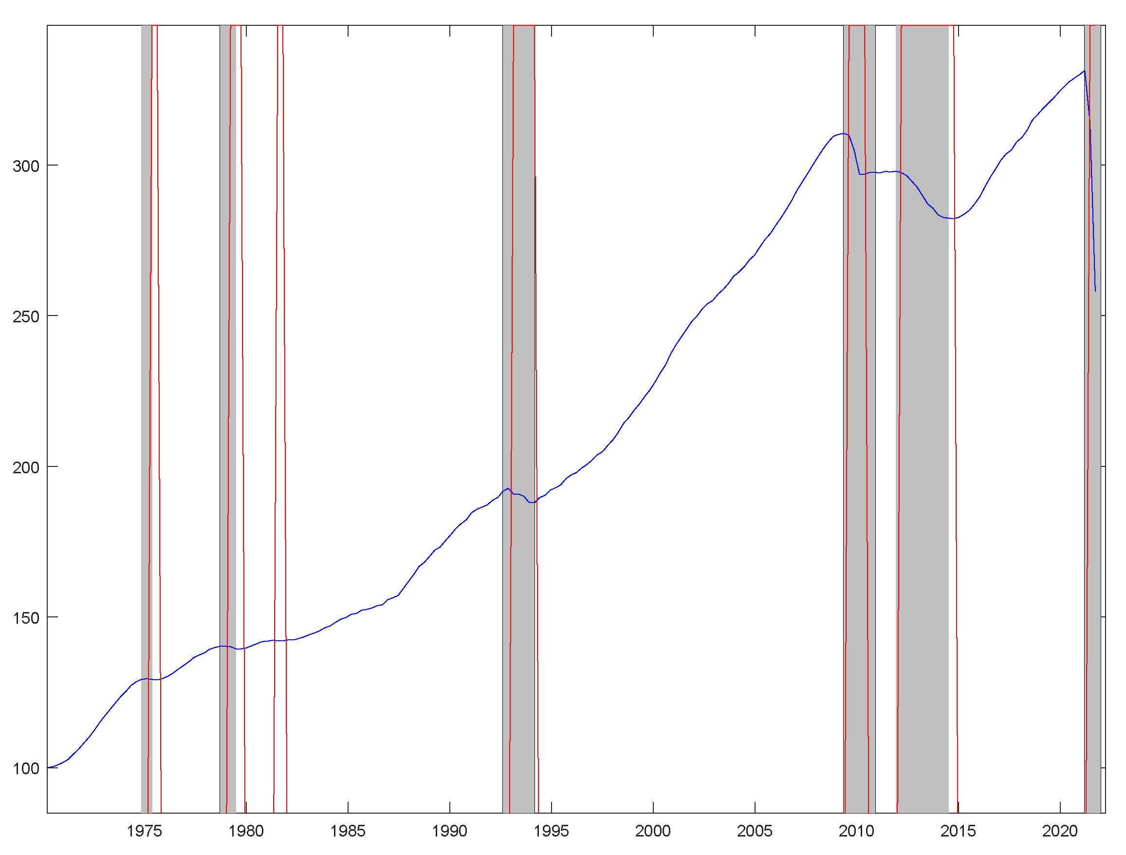
Figure 1 shows that GDP does not increase every single year in Spain. Instead, there are particular identifiable episodes during which GDP sharply falls. The downturns occur at around the periods designated as recessions by the SBCDC, which are marked as shades areas in the graph. (Information about the Committee and the Spanish turning point dates can be found at
http://asesec.org/CFCweb/en/ accessed on 20 May 2021). The committee identified six recessions since the 1970s: the impact of the two oil crises in the 1970s and early 1980s, the brief crisis of the 1990s, the double dip caused by the global financial crisis in 2008 and the European sovereign debt crisis in 2010 and, finally, the economic impact of COVID-19 pandemic. To determine when a particular recession begins and ends, the committee uses judgments and their decisions are, therefore, difficult to replicate.
To overcome this inconvenient, in this paper we date peaks and troughs from economic indicators using the so-called BBQ mechanical algorithm, which is an implementation of the methodology outlined in [
15]. In short, the non-parametric algorithm provides peaks and troughs of a time series by following three steps: (i) it estimates the possible turning points in the series by picking the local maxima and minima; (ii) it ensures alternating the troughs and the peaks; and (iii) it applies a set of censoring of rules that meet pre-determined criteria of the duration and amplitudes of phases and complete cycles. For example, a complete cycle must last four quarters at least. In addition, the minimum duration of a recession is two quarters. To ease of comparison, the peaks and trough dates identified with BBQ are plotted in
Figure 1 as red vertical lines. As can be seen in the figure, there is no instance in which a SBCDC recession is not identified by the BBQ algorithm, which picks up an additional recession at the begging of the eighties.
Although GDP is the most prominent indicator, the committees emphasize that a recession typically implies a downturn that is widespread across the broad economy. Thus, they consider a variety of indicators to determine turning points. In this paper, we have collected a broad set of 51 specific indicators of both aggregate activity and employment, and others of a sectoral nature, which includes both hard and soft indicators.
Table A1 in the
Appendix A shows the details of the definitions and the acronyms that will be used in the rest of the work, as well as the sources and samples. Overall, the sample begins in February 1970 and ends in March 2020, although each series has a different length and combines monthly and quarterly frequencies. The monthly series are transformed into quarterly by taking the average of the corresponding 3 months, although all series have been previously seasonally adjusted to their original frequency.
The specific business cycle turning points have been dated by applying either the BBQ algorithm, when the series have a trend, or the Markov-switching procedure, when they are represented by a composite index or growth rates.
Figure 2 displays the series-specific recessions, where the recession of a time series (in red) is the period from a BBQ peak to a BBQ trough or the periods with a probability of a recession determined by a Markov-switching model is above 0.5. In addition,
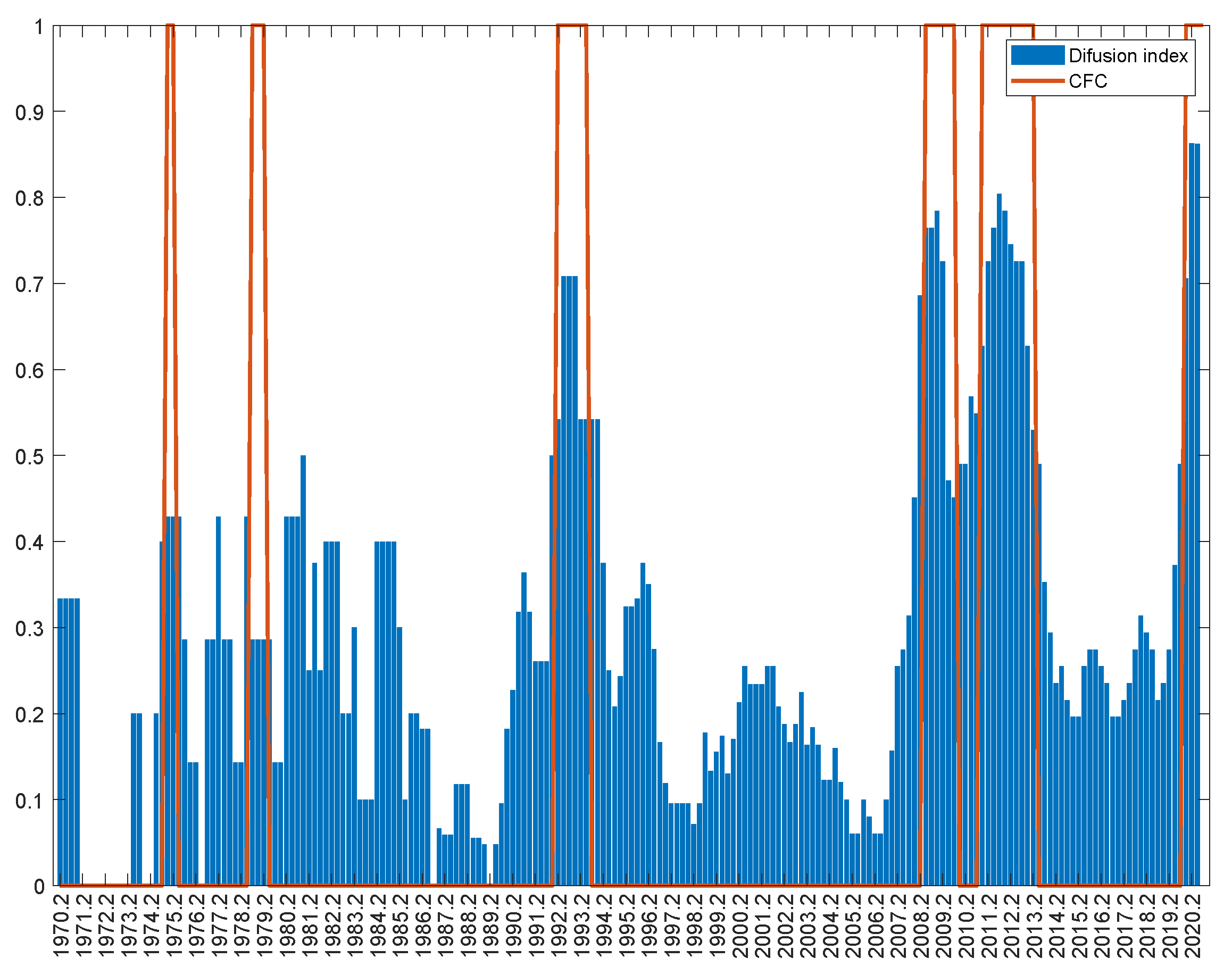
Figure 3 displays the estimated probability that all indicators are in recession in each quarter, adding the SBCDC turning points as red vertical lines.
Summing up, around the dates that the SBCDC identifies recessions there is a wide set of specific indicators that show a recession. However, there are indicators that either advance (usually related to the industrial sector), delay or extend the duration of recessions (for example, those associated with the labor market). Furthermore, not all the specific indicators have the same behavior in each recession.
4.2. Select a Set of Highly Coincident Indicators
Although
Figure 2 and
Figure 3 show that the set of indicators would be useful for ascertaining whether a turning point has occurred, the figures evidence a high dispersion of the specific turning point dates around the beginning and end of the recessions. As the multiple change-point method assumes that the series being dated have been chosen to be coincident indicators, we strongly recommend testing for this in advance by checking how synchronized the cycles are.
For this purpose, we address the issue of synchronization between each indicator and the SBCDC chronology by computing the index of concordance advocated by Harding and Pagan (2002), which measures the percentage of time units spent in the same phase. The index, whose values are plotted in
Figure 4, confirms that there is a relatively high degree of synchronization within the SBCDC business cycles. To ensure strong synchronization, we pick only those indicators for which the concordance index exceeds 90%. Thus, the final set of indicators that exhibit the highest correlation with the SBCDC chronology is formed by six time series:
SSAI,
SAI,
ESIS,
ESIC,
GDP, and
PC. This selection, which combines aggregated, sectorial, and hard and soft indicators, is not very different from the one commonly used by the NBER. Employment indicators are not capable of pinpointing the Spanish cycle since they have a lagging behavior during expansions.
We use the SBCDC chronology to select the coincident indicators, given the high coincidence of the modes detected in the set of indicators and the dating of the committee. Nevertheless, it should be noted that our methodology does not require any prior information or the existence of any dating committee. Alternatively, we could select the optimal set of coincident indicators with a search algorithm applied to different combinations of indicators, where the optimal combination could be selected on the basis of the number of clusters, the entropy, and the variance of the confidence intervals. This procedure could allow us to discard leading or lagging indicators and to choose the combination of indicators that produces the largest modes. Since this option is computationally more expensive, external information of experts, such as that of the SBCDC, can be used to speed up the process.
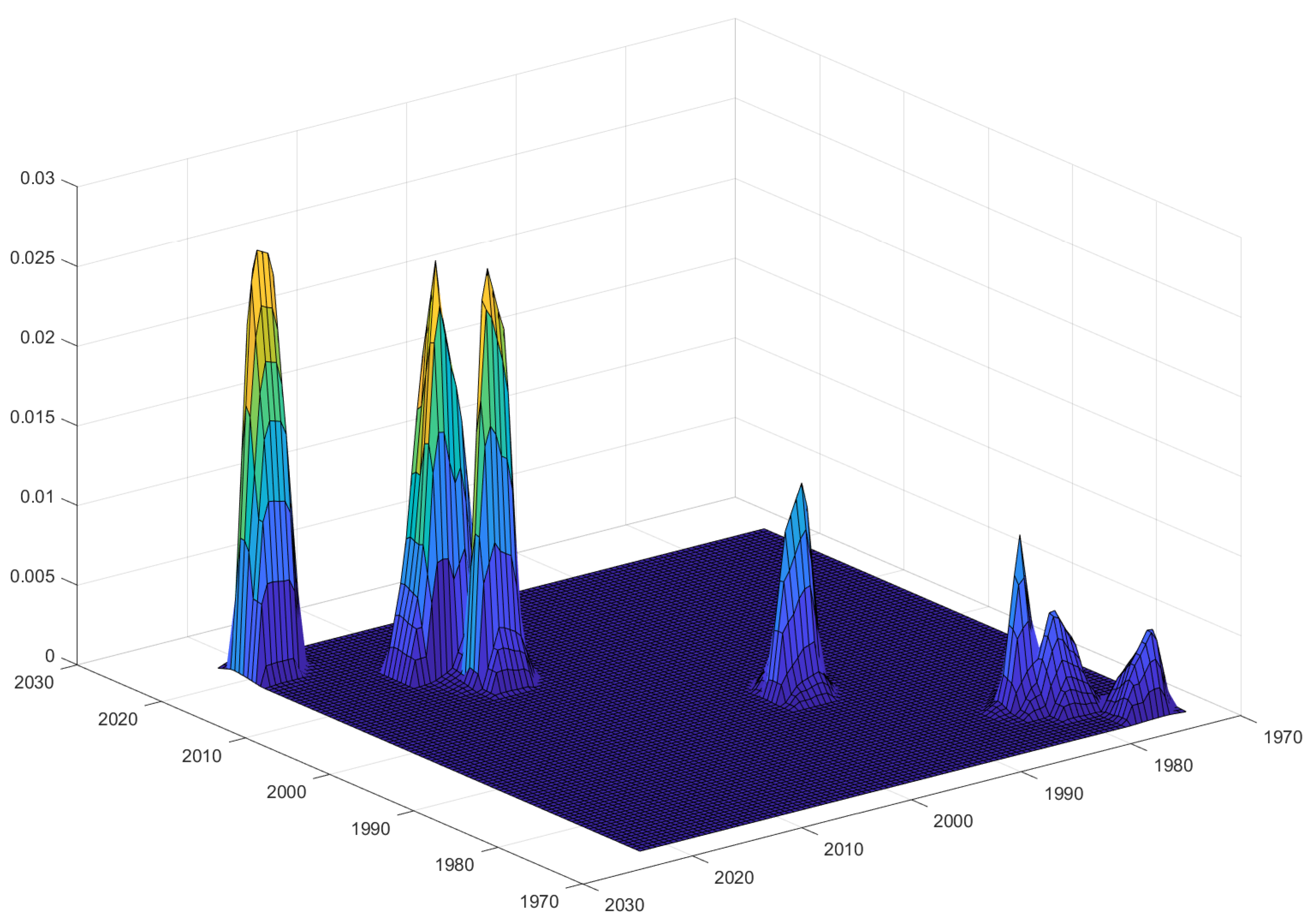
Figure 5 provides a preliminary inspection of the individual chronologies of turning points. In particular, the figure displays the kernel density of the turning points dated with either BBQ or the Markov-switching procedure. The bivariate distribution of the specific peak-trough dates exhibits several modes, which cluster the turning points around the periods of SBCDC-referenced peaks and troughs. In particular, the figure exhibits several modes around the 1970s and the beginning of the 1980s, the early 1990s, the first decade of the new century and, finally, a large concentrated mode at the end of the sample, in 2020. The figure also shows a larger variance of the turning point dates in the 1970s and early 1980s, probably due to the lower quality of the indicators in the late years of Franco’s dictatorship and the unstable political transition towards democracy. By contrast, this figure shows a lower dispersion of the specific turning point dates in the 1990s, around the three modes of the new century related with the double-dip, and in 2020, and the specific turning points shrink toward the modes.
4.3. The Number of Clusters
Prior to determining the number of clusters, we need to specify whether the first phase of reference cycle starts in a recession or an expansion. In our case, we determine that the Spanish economy was in expansion in February 1970 because the first turning point for all the indicators that were available in this period was a peak. In addition, the last turning point in the six indicators is a peak, which implies that the pairs of turning points are not complete. In this case, we create artificial troughs by adding the average duration of the preceding recessions to the peaks.
As a first approximation to the determination of the number of clusters,
Figure 5 suggests that the tentative number of components of the mixture could be six or seven. These numbers refer to the distinct local maxima of the kernel distribution of pairs of peaks and troughs. The main discrepancy between the modes and the SBCDC referenced turning points appears at the end of the 1970s and the early 1980s. This period seems to include an additional cluster.
To formally determine the number of clusters, we estimate mixture models
with different number of clusters
, being the maximum number of clusters
as suggested by visual inspection of the kernel distribution displayed in
Figure 5. For these models, the model selection measures described in
Section 3.3 are computed and the resulting estimates are reported in
Table 1. The first column of the table reveals that the likelihood rises continuously with the number of clusters, reaching a local maximum at
. The algorithm is not able to generate a valid result for
because there are not sufficient numbers of draws to achieve identification.
The results of the penalized classification methods are displayed in columns 2, 3, and 5 of
Table 1. The reported figures show that the local minima of
,
, and
are also achieved for
clusters. According to the figures reported in column 4, the entropy of the model with
clusters is 0, indicating a perfect segmentation of the Spanish cycles. The procedure also takes into account some indicators of the quality of the results. More specifically, we count the percentage of draws in which the algorithm has been unable to generate a bivariate vector of
that complies with the partition constraints of the reference cycle; we check if the estimated
values are within the range of data values allowing a margin of 1 year at the beginning and end; and, finally, we count the percentage of classifications that leave an empty cluster.
Finally, as in [
7], we follow [
11] and compute the Bayes factors sequentially. The sequence of (twice the log of) Bayes factors also points to
as the Bayes factor that establishes the comparison of the model with
clusters and the model with
clusters favors the extra cluster. Although this result does not require prior knowledge of the number of clusters, it is worth noting that the SBCDC establishes
clusters, considering the last peak as an incomplete pair. The difference is found in the late 1970s and early 1980s, a complex period with scarce information, in which the SBCDC chronology establishes 2 recessions, while the specific indicators detect 3 as shown in
Figure 5.
4.4. Estimation of Turning Points
Table 2 shows the results of evaluating our proposal in terms of its ability to capture the turning point dates established by the Spanish Business Cycle Dating Committee. The columns labeled SBCDC and MCPM report the reference cycle dates as determined by the Spanish Business Cycle Dating Committee and our multiple change-point model. The means of the components of the mixtures are estimated using the posterior distributions obtained with the Gibbs rejection sampler algorithm. The BBQ algorithm imposes that a recession should last at least 2 quarters and an expansion, at least 4 quarters. In addition, the table also shows the 95% credible intervals.
The table shows that for each SBCDC-referenced turning point, our mixture model estimates a corresponding turning point, whose credible intervals contain the SBCDC dates in all episodes. Notably, our proposal replicates the SBCDC peaks and troughs very accurately, especially for the turning points dated since the 1990s. However, our method provides an extra pair of turning points at the beginning of the 1980s.
Finally, we address the issue of estimation uncertainty and the misleading signal of turning point dates that some indicators could provide. For this purpose, we focus on the credible intervals, which are the interval within which the estimated turning point dates fall with a particular probability. In our application, the 95% credible intervals provided in
Table 2 are substantially narrow. Given the observed data, the credible intervals indicate that, in the worse-case scenario, the distribution of possible values of the turning point dates have 95% probability of deviating from the estimates only on 1 quarter in the case of peaks and 3 quarters in the case of troughs. This indicates that the method provides very precise estimates of the reference dates and agrees with the view that the economic indicators tend to provide accurate signals of the business cycle turning points.
In particular, the short recession of the 1990s is detected with a delay of a quarter in both the peak and the trough, although the confidence intervals include the exact date provided by the SBCDC. Regarding the global financial crisis, the first impact is identified early in the peak and late in the trough, and something similar occurs with the second blow of the crisis. Finally, the peak that marks the beginning of the crisis caused by the COVID-19 pandemic fully matches that announced by the SBCDC. As expected, the uncertainty in determining the reference dates is a bit larger in the 1970s. In fact, the Committee acknowledges that “Business cycle dating for the period January 1970 (the start of the sample based on available national income accounts at quarterly frequency), until about April 1986 is especially challenging”.
Figure 6 and
Figure 7 display some technical aspects of the estimation process. In particular,
Figure 6 plots the draws of the means and the variances obtained from the replications of the MCMC algorithm. In particular, the two scatter plots of Panel A display the draws for
and
, respectively. In addition, Panel B shows the scatter plots for
. From these scatter plots, it is obvious that the component parameters of the 7 clusters do not differ in the variances but in the means. In addition, the estimated clusters provide a clear segmentation of the time span, which agrees with the restrictions imposed in the Markov-switching transitions. Interestingly, we find that the changes from one cluster to the following one occur very close to the SBCDC-designated pairs of peaks and troughs.
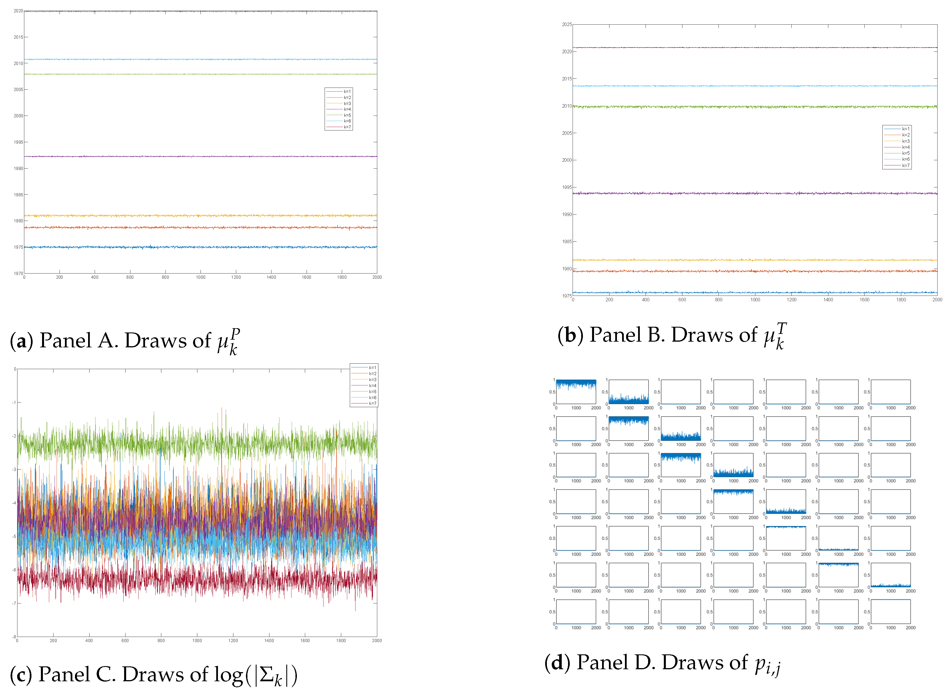
To provide a diagnosis of potential divergent transitions in the MCMC filter, we plot in
Figure 7 the estimated parameter values for each iteration of the filter. In particular, the figure displays the conditional plots of the peaks
(Panel A), the troughs
(Panel B), the variances
(Panel C), and the transition probabilities
and
(Panel D) for each of the
components of the mixture model. In all of these cases, the rejection sampler seems to mix well because the trace plots of the parameter estimates converge to their respective posterior distributions at the initial labeling.
In addition, we computed the Gelman–Rubin scale reduction factor diagnostic corrected by accounting for sampling variability, usually known as Rc. In our context, all the Gelman–Rubin diagnostics were 1 (or very close to one). More importantly, the maximum Rc was less than 1.1, which indicated that no convergence issues were detected.
Finally,
Figure 8 displays the classification probabilities, which are estimated as the number of times that a particular observation is classified in each of the 7 cluster across the replication of the MCMC sampler. The figure shows a high classification performance of the model because the classification probabilities stay close to 1 at about each of the seven pairs of peak-trough dates established by the SBCDC business cycle committee, providing a clear segmentation of the Spanish reference cycle.
5. Conclusions
This paper provides an automatic procedure to date the reference cycle turning points in Spain. Based on the novel methodology proposed by [
4], the turning points obtained from a set of economic indicators are assumed to be realizations of a restricted Markov-switching Gaussian mixture model, where the means of the model components are viewed as the reference cycle peak-trough dates. This approach is equivalent to considering a multiple change-point model where the reference cycle is a collection of increasing change-points (peak-trough dates) that segment the time span into K non-overlapping episodes. The computation is carried out with Bayesian techniques using a Markov Chain Monte Carlo (MCMC) algorithm which is implemented using the Gibbs sampler.
The application comprises several steps. Firstly, we collect a broad set of specific indicators that includes aggregate and sectorial variables, both hard and soft. Secondly, we compute the turning points of each individual indicator by using the quarterly Bry–Boschan method and analyze carefully their behavior with respect to the business cycle. A search algorithm using the concordance index allows us to find the optimal set of coincident indicators and build the database of peak-trough pairs. Thirdly, we select the number of clusters through several measures based on the likelihood function and Bayesian criteria. Finally, we estimate the turning points as the mean of the draw distribution for each cluster and then compute their confidence intervals.
The method identifies seven recessions in the period from February 1970 to February 2020. Three of these recessions are dated in the 1970s and early 1980s. It also dates the recession of the 1990s, the double-dip of the global financial crisis and the sovereign debt crisis in the first two decades of the 21st century and, finally, the recent hit of the COVID-19 pandemic. These results show the good performance of the model provide estimates of the Spanish turning point dates, which are in close agreement to those established by the Spanish Business Cycle Dating Committee (SBCDC). In fact, since the nineties there has been an almost perfect coincidence of the timings. The greatest discrepancies occurred in the 1970s and early 1980s, a turbulent period in Spain characterized by the juxtaposition of the successive oil crises and the political transition of the 1970s together with the scarcity of statistical sources.
Summing up, the method proposed by Camacho et al. (2021) has successfully overcome the challenge of producing a credible chronology of the reference cycle of the Spanish economy using automatic rules based on a set of specific indicators. It is, therefore, a useful instrument that complements the work carried out by the Spanish Business Cycle Dating Committee and that can be used by both policy-makers and academics interested in analyzing the economic cycle in Spain.
Author Contributions
Conceptualization, M.C., M.D.G. and A.G.-L.; methodology, M.C. and M.D.G.; software, M.C. and M.D.G.; validation, M.C., M.D.G. and A.G.-L.; formal analysis, M.C. and M.D.G.; investigation, M.C., M.D.G. and A.G.-L.; resources, M.C., M.D.G. and A.G.-L.; data curation, M.C., M.D.G. and A.G.-L.; writing—original draft preparation, M.C., M.D.G. and A.G.-L.; writing—review and editing, M.C., M.D.G. and A.G.-L.; visualization, M.C., M.D.G. and A.G.-L.; supervision, M.C., M.D.G. and A.G.-L.; project administration, M.C., M.D.G. and A.G.-L.; funding acquisition, M.C., M.D.G. and A.G.-L. All authors have read and agreed to the published version of the manuscript.
Funding
This research was funded by the support of grants PID2019-107192GB-I00 (AEI/10.13039/ 501100011033) and 19884/GERM/15, and ECO2017-83255-C3-1-P and ECO2017-83255-C3-3-P (MICINU, AEI/ERDF, EU), respectively. Data and codes that replicate our results are available from the authors’ websites. The views in this paper are those of the authors and do not represent the views of the Banco de España, the Eurosystem, or the Spanish Business Cycle Dating Committee.
Institutional Review Board Statement
Not applicable.
Informed Consent Statement
Not applicable.
Data Availability Statement
A detailed description of the data sources used can be found in
Appendix A.
Conflicts of Interest
The authors declare no conflict of interest. The funders had no role in the design of the study; in the collection, analyses, or interpretation of data; in the writing of the manuscript, or in the decision to publish the results.
Appendix A
Table A1.
Variable definitions.
Table A1.
Variable definitions.
| Variable | Acronym | Source | Sample |
|---|
| Gross Domestic Product | GDP | National Statistics Institute (INE) | 1970:I-2020:II |
| Private consumption | PC | INE | 1995:I-2020:II |
| Labor force | LF | INE | 1972:III-2020:II |
| Female labor force | FLF | INE | 1972:III-2020:II |
| Unemployment rate | UR | INE | 1989:01-2020:07 |
| Social Security registrations | SSR | Ministerio de Inclusión, Seguridad
Social y Migraciones | 1982:01-2020:09 |
| Social Security registrations without workers on furlough | SSRwF | Ministerio de Inclusión, Seguridad Social y Migraciones | 1982:01-2020:09 |
| Electricity consumption | EC | Red eléctrica de España | 1981:01-2020:08 |
| Big firms sales | BFS | Agencia Tributaria | 1996:01-2020:07 |
| Retail trade index | RTI | INE | 1995:01-2020:06 |
| Industrial production index | IPI | INE | 1975:01-2020:08 |
| Private vehicles registration | PVR | Asociación Española de Fabricantes de Automóviles y Camiones (ANFAC) | 1975:01-2020:07 |
| Services sector activity index | SSAI | INE | 2000:01-2020:07 |
| Cement consumption | CC | Oficemen | 1989:02- 2020:05 |
| New construction permits | PT | Ministerio de Transportes, movilidad y agenda urbana | 1992:01-2020:07 |
| Home sales | HS | INE | 2007:01-2020:08 |
| Mortgages | M | INE | 2003:01-2020:07 |
| Business turnover index | BTI | INE | 2002:01-2020:05 |
| Exports | EX | Departamento de Aduanas y Ministerio de Asuntos Económicos y Transformación Digital | 1970:06-2020:05 |
| Imports | IM | Departamento de Aduanas y Ministerio de Asuntos Económicos y Transformación Digital | 1970:06-2020:05 |
| Overnight tourist stays | OTS | INE | 1995:01-2020:09 |
| Tourist arrivals | TA | INE | 1995:01-2020:09 |
| Productive capacity utilization | PCU | Ministerio de Asuntos Económicos y Transformación Digital | 1995:I-2020:III |
| Synthetic activity indicator | SAI | EDE Business | 1995:01-2020:06 |
| Synthetic activity indicator. Industry | SAII | EDE Business | 1995:01-2020:06 |
| Synthetic activity indicator. Construction | SAIC | EDE Business | 1995:01-2020:06 |
| Synthetic activity indicator. Construction investment | SAICI | EDE Business | 1995:01-2020:06 |
| Synthetic activity indicator. Services | SAIS | EDE Business | 1995:01-2020:06 |
| Synthetic consumption indicator | SCI | Ministerio de Asuntos Económicos y Transformación Digital | 1995:01-2020:06 |
| Synthetic consumption indicator. Large chain stores | SCIL | Ministerio de Asuntos Económicos y Transformación Digital | 1995:01-2020:06 |
| Composite produce manager index | PMI Comp | IHS Markit | 1999:08-2020:06 |
| Economic sentiment indicator | ESI | European Commission | 1987:04-2020:10 |
| Economic sentiment indicator. Industry | ESII | European Commission | 1987:04-2020:08 |
| Economic sentiment indicator. Services | ESIS | European Commission | 1996:01-2020:08 |
| Economic sentiment indicator. Consumption | ESIC | European Commission | 1986:06-2020:08 |
| Economic sentiment indicator. Retail | ESIR | European Commission | 1988:01-2020:08 |
| Economic sentiment indicator. Building | ESIB | European Commission | 1989:01-2020:08 |
| Employment expectations indicator | EEI | Eurostat | 1996:01-2020:08 |
| Consumer confidence index | CCI | Centro de investigaciones sociológicas (CIS) | 2004:09-2020:10 |
| Credit to households (% GDP) | CH | Banco de España | 1995:IV-2020:IV |
| Credit to Non Financial Corporate (% GDP) | HHRBD | Banco de España | 1995:IV-2020:IV |
| Ratio of households debt over disposable income | HHGDP | Banco de España | 1987:I-2020:II |
| Ratio of households debt over GDP | CNFC | Banco de España | 1987:I-2020:II |
| Ratio of non financial corporate debt over GDP | NFCDGDP | Banco de España | 1987:I-2020:II |
| Ratio of non performing housing loans | NPHL | Banco de España | 1998:IV-2020:II |
| Ratio of non performing durable consumption loans | NPDCL | Banco de España | 1998:IV-2020:II |
| Ratio of non performing production activities loans | NPPAL | Banco de España | 1998:IV-2020:II |
| Sovereign risk premia ES-DE | SRP | Datastream | 1991:07-2020:09 |
| IBEX 35 index | IBEX | Datastream | 1987:01-2020:09 |
| EA Gross Domestic Product | EAGDP | Eurostat | 1995:I-2020:II |
| VIX index | VIX | Datastream | 1990:01-2020:09 |
References
- Burns, A.; Mitchell, W. Measuring Business Cycles; National Bureau of Economic Research: New York, NY, USA, 1946. [Google Scholar]
- Chauvet, M.; Piger, J. A comparison of the real-time performance of business cycle dating methods. J. Bus. Econ. Stat. 2008, 26, 42–49. [Google Scholar] [CrossRef] [Green Version]
- Harding, D.; Pagan, A. Synchronization of cycles. J. Econ. 2006, 132, 59–79. [Google Scholar] [CrossRef]
- Harding, D.; Pagan, A. The Econometric Analysis of Recurrent Events in Macroeconomics and Finance; Princeton University Press: Princeton, NJ, USA, 2016. [Google Scholar]
- Stock, J.; Watson, M. Indicators for dating business cycles: Cross-history selection and comparisons. Am. Econ. Rev. Pap. Proc. 2010, 100, 16–19. [Google Scholar] [CrossRef] [Green Version]
- Stock, J.; Watson, M. Estimating turning points using large data sets. J. Econ. 2014, 178, 368–381. [Google Scholar] [CrossRef]
- Camacho, M.; Gadea, M.D.; Gomez-Loscos, A. A new approach to dating the reference cycle. J. Bus. Econ. Stat. 2021. [Google Scholar] [CrossRef]
- Bry, G.; Boschan, C. Cyclical Analysis of Time Series: Procedures and Computer Programs; National Bureau of Economic Research: New York, NY, USA, 1971. [Google Scholar]
- Hamilton, J. A new approach to the economic analysis of nonstationary time series and the business cycles. Econometrica 1989, 57, 357–384. [Google Scholar] [CrossRef]
- Albert, J.; Chib, S. Bayes inference via Gibbs sampling of autoregressive time series subject to Markov mean and variance shifts. J. Bus. Econ. Stat. 1993, 11, 1–15. [Google Scholar]
- Chib, S. Estimation and comparison of multiple change-point models. J. Econ. 1998, 86, 221–241. [Google Scholar] [CrossRef]
- Frühwirth-Schnatter, S. Finite Mixture and Markov Switching Models; Springer Series in Statistics; Springer: New York, NY, USA, 2006. [Google Scholar]
- Fraley, C.; Raffery, A.E. Model-Based Clustering, Discriminant Analysis, and Density Estimation. J. Am. Econ. Assoc. 2002, 97, 611–631. [Google Scholar] [CrossRef]
- Kass, R.; Raftery, A. Bayes factors. J. Ame. Stat. Assoc. 1995, 90, 773–795. [Google Scholar] [CrossRef]
- Harding, D.; Pagan, A. Dissecting the cycle: A methodological investigation. J. Mon. Econ. 2002, 49, 365–381. [Google Scholar] [CrossRef]
Figure 1.
Business cycle SBCDC. Notes: This figure displays with grey shadow bars the recessions established by the Spanish Business Cycle Dating Committee (SBCDC). The vertical red lines represent the peaks and troughs detected by the BBQ applied to the GDP. Finally, the blue line shows the evolution of GDP.
Figure 2.
Heat map of specific indicators. Notes: This figure represents the periods of expansion (blue) and recession (garnet) for each specific indicator. The switch of the states has been determined from the turning points computed with the Bry–Boschan algorithm.
Figure 2.
Heat map of specific indicators. Notes: This figure represents the periods of expansion (blue) and recession (garnet) for each specific indicator. The switch of the states has been determined from the turning points computed with the Bry–Boschan algorithm.
Figure 3.
Diffusion index of specific indicators. Notes: The blue bars show the percentage of series that are in recession in each period. The garnet boxes represent the recessions established by the Spanish Business Cycle Dating Committee (SBCDC).
Figure 3.
Diffusion index of specific indicators. Notes: The blue bars show the percentage of series that are in recession in each period. The garnet boxes represent the recessions established by the Spanish Business Cycle Dating Committee (SBCDC).
Figure 4.
Concordance index of specific indicators. Notes: This figure displays the concordance index of each indicator and the business cycle established by the Spanish Business Cycle Dating Committee (SBCDC). The garnet line corresponds with a value of 0.9.
Figure 4.
Concordance index of specific indicators. Notes: This figure displays the concordance index of each indicator and the business cycle established by the Spanish Business Cycle Dating Committee (SBCDC). The garnet line corresponds with a value of 0.9.
Figure 5.
Bivariate distribution of specific turning point dates. Notes: The figure plots the bivariate kernel density of the specific pairs of peak-trough dates.
Figure 5.
Bivariate distribution of specific turning point dates. Notes: The figure plots the bivariate kernel density of the specific pairs of peak-trough dates.
Figure 6.
Scatter plots of means and variances. Notes: The figure plots the scatter plots of conditional draws of the MCMC sampler for and (Panel A) and (Panel B) for each of the clusters.
Figure 6.
Scatter plots of means and variances. Notes: The figure plots the scatter plots of conditional draws of the MCMC sampler for and (Panel A) and (Panel B) for each of the clusters.
Figure 7.
Diagnosis of the Gibbs sampler. Notes: The figure plots the trace plots of the MCMC draws for (Panel A), (Panel B), (Panel C), and (Panel D) for each of the clusters.
Figure 7.
Diagnosis of the Gibbs sampler. Notes: The figure plots the trace plots of the MCMC draws for (Panel A), (Panel B), (Panel C), and (Panel D) for each of the clusters.
Figure 8.
Classification probabilities. Notes: The figure plots the estimates of , for and from January 1959 to August 2010.
Figure 8.
Classification probabilities. Notes: The figure plots the estimates of , for and from January 1959 to August 2010.
Table 1.
Results of selection of K.
Table 1.
Results of selection of K.
| K | LogLik | AIC | BIC | Entropy | BIC-Entropy | Bayes Factor (k = i/k = i+ 1) |
|---|
| 1 | −2229.78 | 4469.57 | 4486.30 | - | - | - |
| 2 | −696.46 | 1414.91 | 1451.73 | 0.03 | 1451.80 | 3034.57 |
| 3 | −400.14 | 834.27 | 891.18 | 0.00 | 891.18 | 560.55 |
| 4 | −141.25 | 328.51 | 405.49 | 0.00 | 405.50 | 485.69 |
| 5 | −25.28 | 108.57 | 205.63 | 0.00 | 205.63 | 199.86 |
| 6 | 13.64 | 42.72 | 159.87 | 0.00 | 159.87 | 45.76 |
| 7 | 42.61 | −3.22 | 134.01 | 0.00 | 134.01 | 25.86 |
| 8 | - | - | - | - | - | - |
Table 2.
Results of empirical illustration (K = 7).
Table 2.
Results of empirical illustration (K = 7).
| SBCDC | MCPM | Deviation (in Quarters) |
|---|
| Peaks | Troughs | Peaks | Troughs | Peaks | Troughs |
| 1974.4 | 1975.2 | 1974.4 | 1975.3 | 0 | 1 |
| | | (1974.4, 1975.1) | (1975.3, 1975.4) | | |
| 1978.3 | 1979.2 | 1978.3 | 1979.3 | 0 | 1 |
| | | (1978.3, 1978.4) | (1979.2, 1979.3) | | |
| - | - | 1980.4 | 1981.3 | - | - |
| | | (1980.4, 1981.1) | (1981.3, 1981.4) | | |
| 1992.1 | 1993.3 | 1992.2 | 1993.4 | 1 | 1 |
| | | (1992.1, 1992.2) | (1993.3, 1994.1) | | |
| 2008.2 | 2009.4 | 2007.4 | 2009.4 | −2 | 0 |
| | | (2007.4, 2007.4) | (2009.3, 2009.4) | | |
| 2010.4 | 2013.2 | 2010.3 | 2013.3 | −1 | 1 |
| | | (2010.3, 2010.4) | (2013.3, 2013.4) | | |
| 2019.40 | - | 2019.4 | - | 0.00 | - |
| | | (2019.4, 2019.4) | (-,-) | | |
| Publisher’s Note: MDPI stays neutral with regard to jurisdictional claims in published maps and institutional affiliations. |
© 2021 by the authors. Licensee MDPI, Basel, Switzerland. This article is an open access article distributed under the terms and conditions of the Creative Commons Attribution (CC BY) license (https://creativecommons.org/licenses/by/4.0/).


