Global Dynamics of an SEIR Model with the Age of Infection and Vaccination

Abstract

This paper is concerned with the stability of a SEIR (susceptible-exposed-infectious-recovered) model with the age of infection and vaccination. Firstly, we prove the positivity, boundedness, and asymptotic smoothness of the solutions. Next, the existence and local stability of disease-free and endemic steady states are shown. The basic reproduction number $R_0$ is introduced. Furthermore, the global stability of the disease-free and endemic steady states is derived. Numerical simulations are shown to illustrate our theoretical results.

1. Introduction

Epidemic models are important tools for helping people fight against infectious diseases. Epidemic models that are constructed under reasonable assumptions can help people. For example, it was predicted that only a limited number of people would be infected by the Severe Acute Respiratory Syndrome (SARS) in 2003 before it disappeared. Epidemic models can also help people to prevent and control an infectious disease by analyzing the variables and the basic reproduction numbers. They are important tools in the ongoing fight against COVID-19.

A large number of models, such as susceptible-infectious-recovered (SIR) models (see [1]), SIS models, SIRS models (see [2,3,4]), SEI models (see [5]), SEIR models, and other models (see [6]) were recently studied. Rost and Wu [7] constructed a SEIR model that took consideration of the impact of infection age. As (chronological or infection) age is an important factor in population dynamics, many researchers investigated models with age (see [8,9,10,11,12,13,14,15,16,17,18]), thus addressing the stability of steady states, and even bifurcation analyses (see [19]).

Although vaccines were successfully produced to fight against many diseases, such as COVID-19, it is still unclear whether or not the diseases will disappear. In [20], Posny et al. presented an epidemiological model of cholera and used the variable $V(t)$ to denote vaccinated individuals. In [14], Lin et al. extended the model in [20] to the following differential equations:

$$\begin{array}{c}\hfill \dot{S}(t)=A-(\mu +\varphi )S(t)-S(t)({\int }_0^{\infty }\frac{{\beta }_1(a)i(a,t)}{1+\alpha i(a,t)}da+{\int }_0^{\infty }\frac{{\beta }_2(b)p(b,t)}{k+p(b,t)}db),\end{array}$$

(1a)

$$\begin{array}{c}\hfill \dot{V}(t)=\varphi S(t)-\mu V(t)-\sigma V(t)({\int }_0^{\infty }{\beta }_1(a)i(a,t)da+{\int }_0^{\infty }\frac{{\beta }_2(b)p(b,t)}{k+p(b,t)}db),\end{array}$$

(1b)

$$\begin{array}{c}\hfill \frac{\partial i(a,t)}{\partial t}+\frac{\partial i(a,t)}{\partial a}=-\theta (a)i(a,t),\end{array}$$

(1c)

$$\begin{array}{c}\hfill \dot{R}(t)={\int }_0^{\infty }\gamma (a)i(a,t)da-\mu R(t),\end{array}$$

(1d)

$$\begin{array}{c}\hfill \frac{\partial p(b,t)}{\partial t}+\frac{\partial p(b,t)}{\partial b}=-{\delta }_p(b)p(b,t),\end{array}$$

(1e)

with the boundary conditions

$$\begin{array}{c}\hfill i(0,t)=(S(t)+\sigma V(t))({\int }_0^{\infty }\frac{{\beta }_1(a)i(a,t)}{1+\alpha i(a,t)}da+{\int }_0^{\infty }\frac{{\beta }_2(b)p(b,t)}{k+p(b,t)}db),t>0,\end{array}$$

(2a)

$$\begin{array}{c}\hfill p(0,t)={\int }_0^{\infty }\xi (a)i(a,t)da,t>0,\end{array}$$

(2b)

where $S(t),V(t),R(t)$ are the densities of susceptible, vaccinated, and recovered individuals at time t, respectively. $i(a,t)$ is the density of infected individuals with infection age a at time t. $p(b,t)$ is the concentration of V. Cholera with biological age b at time t. The saturation infection rate is $\frac{{\beta }_1(a)i(a,t)}{1+\alpha i(a,t)}$. Other parameters are listed in Table 1 in [14].

Based on the above motivations, in the present paper, we extend the model in [14,20] by considering exposed individuals and taking a general incidence rate with $f(S)g(I)$ to make our model applicable to more cases. We propose the following SEIR model with the age of infection and vaccination:

$$\begin{array}{c}\hfill \dot{S}(t)=A-(\mu +\varphi )S(t)-f(S(t)){\int }_0^{\infty }\beta (a)g(i(a,t))da,\end{array}$$

(3a)

$$\begin{array}{c}\hfill \dot{V}(t)=\varphi S(t)-\mu V(t)-\sigma V(t){\int }_0^{\infty }\beta (a)g(i(a,t))da,\end{array}$$

(3b)

$$\begin{array}{c}\hfill \dot{E}(t)=(f(S(t))+\sigma V(t)){\int }_0^{\infty }\beta (a)g(i(a,t))da-\mu E(t)-\omega E(t),\end{array}$$

(3c)

$$\begin{array}{c}\hfill \frac{\partial i(a,t)}{\partial t}+\frac{\partial i(a,t)}{\partial a}=-(\mu +\gamma (a)+\rho (a))i(a,t),\end{array}$$

(3d)

$$\begin{array}{c}\hfill \dot{R}(t)={\int }_0^{\infty }\gamma (a)i(a,t)da-(\mu +\delta )R(t),\end{array}$$

(3e)

with the boundary condition

$$i(0,t)=\omega E(t)+\delta R(t).$$

(4)

We denote its initial condition as

$$\begin{array}{ccc}\hfill X_0:& =& (S(0),V(0),E(0),i(·,0),R(0))\hfill \\ & =& (S_0,V_0,E_0,i_0(·),R_0)\in {\mathbb{R}}^{+}\times {\mathbb{R}}^{+}\times {\mathbb{R}}^{+}\times {\mathbf{L}}_{+}^1(0,\infty )\times {\mathbb{R}}^{+},\hfill \end{array}$$

(5)

where $S(t)$, $V(t)$, $E(t)$, and $R(t)$ denote the numbers of susceptible, vaccinated, exposed, and recovered individuals at time t; $i(a,t)$ is the number of infected individuals with infection age a at time t. ${\mathbf{L}}_{+}^1(0,\infty )$ represents the set of all integrable functions from $(0,\infty )$ to ${\mathbb{R}}^{+}=[0,\infty )$. Parameter A is the recruitment rate of susceptible individuals. Individuals in each compartment die at rate $\mu$. Susceptible individuals are infected by infected individuals with age of infection a at rate $\beta (a)$. Exposed individuals are transferred into the infected group at a constant rate of $\omega$. Infected individuals with age of infection a are recovered at rate $\gamma (a)$ and revert to the infected group at a constant rate $\delta$. $\rho (a)$ is the disease-induced death rate of infectious individuals. $\varphi$ is the vaccination rate of susceptible individuals. The vaccinated individuals revert to the susceptible group at a constant rate $\sigma$ due to the imperfect efficiency of vaccination. The state space of the model (3a–e) is

$$X^{+}={\mathbb{R}}^{+}\times {\mathbb{R}}^{+}\times {\mathbb{R}}^{+}\times {\mathbf{L}}_{+}^1(0,\infty )\times {\mathbb{R}}^{+}$$

with the norm

$$\Vert (S,V,E,i,R)\Vert :=\mid S\mid +\mid V\mid +\mid E\mid +{\int }_0^{\infty }i(a,·)da+\mid R\mid .$$

We make the following assumptions for the functions $\beta (·),\gamma (·),\rho (·)$.

Assumption 1.

$\beta (·),\gamma (·),$ and $\rho (·)$ satisfy the following properties:

(i) 

$\beta (·)$ is Lipschitz continuous on ${\mathbb{R}}^{+}$ with the Lipschitz coefficient $L_{\beta }$.

(ii) 

$\beta (·),\gamma (·),\rho (·)\in {\mathbf{L}}_{+}^1(0,\infty )$.

(iii) 

We denote $\widehat{\beta },\widehat{\gamma }$, and $\widehat{\rho }$ as the essential supremums of $\beta (·),\gamma (·)$, and $\rho (·)$, respectively.

Assumption 2.

Assume that

(i) 

$f(x)\ge 0$, $g(x)\ge 0$.

(ii) 

$f(x)=0$ or $g(x)=0$ if and only if $x=0$.

(iii) 

$f^{{}^{\prime }}(x)>0,g^{{}^{\prime }}(x)>0$ and $f^{″}(x)\le 0,g^{″}(x)\le 0$.

Our model (3a–e) extends and generalizes several recent works. These revisions bring challenges in the analysis, such as in the analysis of the well-posedness and in the construction of suitable Lyapunov functionals. Therefore, our work is meaningful and useful for people who study these kinds of models. The obtained results may lead to better understanding of the transmission of infectious diseases with consideration of vaccination. This paper is organized as follows: in Section 2, we identify the dissipativeness, positivity, and asymptotic smoothness of the solutions of the model; Section 3 is devoted to the existence and local stability of the disease-free and endemic steady states, and the calculation of the basic reproduction number; in Section 4, we establish the global stability of the equilibrium by constructing suitable Lyapunov functionals; next, numerical simulations are performed to verify the validity of our main theoretical results, and finally, the paper ends with a brief conclusion.

2. Preliminaries

Let $(S(t),V(t),E(t),i(a,t),R(t))$ be a solution of system (3a–e) satisfying the boundary condition (4) and the initial condition (5). For convenience, we denote

$$\psi (a)=e^{-{\int }_0^a(\mu +\gamma (u)+\rho (u))du}.$$

(6)

Solving Equation (3c) by integrating it along the characteristic lines $t-a=const$, we have

$$i(a,t)=\left\{\begin{array}{ccc}\hfill (\omega E(t-a)+\delta R(t-a))\psi (a),& & 0\le a<t,\hfill \\ \hfill i_0(a-t)\frac{\psi (a)}{\psi (a-t)},& & 0\le t\le a.\hfill \end{array}\right.$$

(7)

2.1. Positivity and Boundedness of Solutions

From Equation (7), $i(a,t)$ remains positive for all $t\ge 0$. From Equation (3a), $S(t)$ remains positive for all $t\ge 0$, since $\dot{S}(t^{*})=A>0$ for all $t^{*}$ satisfying $S(t^{*})=0$. Similarly, $V(t)$, $R(t)$, and $E(t)$ remain positive for all $t\ge 0$.

We denote

$$\mathsf{\Omega }=\left\{(x,v,y,z,\psi )\in X^{+}|\Vert (x,v,y,z,\psi )\Vert \le max\{\frac{A}{\mu },\Vert x_0\Vert \}\right\}.$$

Using the standard theory in [21], the system (3a–e) with (4) and (5) has a unique non-negative solution on ${\mathbb{R}}^{+}$. We define a continuous semiflow, which is denoted as $\mathsf{\Phi }:{\mathbb{R}}^{+}\times X^{+}\to X^{+}$.

$$\mathsf{\Phi }(t,x_0)=(S(t),V(t),E(t),i(·,t),R(t)),t\in {\mathbb{R}}^{+},x_0\in X^{+}.$$

Then, we have

$$\Vert \mathsf{\Phi }(t,x_0)\Vert =\Vert (S,V,E,i,R)\Vert =S(t)+V(t)+E(t)+{\int }_0^{\infty }i(a,t)da+R(t).$$

(8)

Proposition 1.

For system (3a–e)–(5), the following statements hold true.

(a) 

Ω is positively invariant for Φ, i.e., $\mathsf{\Phi }(t,x_0)\in \mathsf{\Omega }$ for all $t\ge 0,x_0\in \mathsf{\Omega }$;

(b) 

Φ is point dissipative, and Ω attracts all points in $X^{+}$.

Proof. 

From Equation (8), we have

$$\begin{array}{ccc}\hfill & & \frac{d}{dt}\Vert \mathsf{\Phi }(t,x_0)\Vert \hfill \\ & =& \frac{dS(t)}{dt}+\frac{dV(t)}{dt}+\frac{dE(t)}{dt}+\frac{d}{dt}{\int }_0^{\infty }i(a,t)da+\frac{dR(t)}{dt}\hfill \\ & =& \frac{dS(t)}{dt}+\frac{dV(t)}{dt}+\frac{dE(t)}{dt}+{\int }_0^{\infty }\frac{\partial i(a,t)}{\partial t}da+\frac{dR(t)}{dt}.\hfill \end{array}$$

(9)

It follows from system (3a–e) that

$$\begin{array}{ccc}\hfill & & \frac{d}{dt}\Vert \mathsf{\Phi }(t,x_0)\Vert \hfill \\ & =& \frac{dS(t)}{dt}+\frac{dV(t)}{dt}+\frac{dE(t)}{dt}+\frac{dR(t)}{dt}\hfill \\ & & +{\int }_0^{\infty }[-(\mu +\gamma (a)+\rho (a))i(a,t)-\frac{\partial i(a,t)}{\partial a}]da\hfill \\ & =& \frac{dS(t)}{dt}+\frac{dV(t)}{dt}+\frac{dE(t)}{dt}+\frac{dR(t)}{dt}\hfill \\ & & -{\int }_0^{\infty }{(\mu +\gamma (a)+\rho (a))i(a,t)da-i(a,t)|}_0^{\infty }\hfill \\ & =& A-\mu S(t)-\mu V(t)-\mu E(t)-\omega E(t)-{\int }_0^{\infty }\rho (a)i(a,t)da\hfill \\ & & -{\int }_0^{\infty }{\mu i(a,t)da-(\mu +\delta )R(t)-i(a,t)|}_0^{\infty }.\hfill \end{array}$$

(10)

Substituting Equation (4) into Equation (10), we have

$$\begin{array}{ccc}\hfill & & \frac{d}{dt}\Vert \mathsf{\Phi }(t,x_0)\Vert \hfill \\ & =& A-\mu S(t)-\mu V(t)-\mu E(t)-\mu R(t)\hfill \\ & & -{\int }_0^{\infty }\mu i(a,t)da-{\int }_0^{\infty }\rho (a)i(a,t)da\hfill \\ & \le & A-\mu \Vert \mathsf{\Phi }(t,x_0)\Vert .\hfill \end{array}$$

(11)

Solving Equation (11), we have

$$\Vert \mathsf{\Phi }(t,x_0)\Vert \le \frac{A}{\mu }-e^{-\mu t}(\frac{A}{\mu }-\Vert x_0\Vert ),$$

which implies

$$\Vert \mathsf{\Phi }(t,x_0)\Vert \le max\{\frac{A}{\mu },\Vert x_0\Vert \}$$

for all $t\ge 0$. This completes the proof. □

From Proposition 1, we have the following results.

Proposition 2.

There exists some constant $M>\frac{A}{\mu }$ such that

$$\begin{array}{cc}\hfill & S(t)\le M,V(t)\le M,E(t)\le M,\\ & {\int }_0^{\infty }i(a,t)da\le M,R(t)\le M\end{array}$$

(12)

hold true for all $t\ge 0$ if $x_0\in X^{+}$ and $\Vert x_0\Vert \le M$.

Proposition 3.

Define a bounded set $C\in X^{+}$. Then,

(i) 

${\mathsf{\Phi }}_t(C)$ is bounded;

(ii) 

${\mathsf{\Phi }}_t$ is eventually bounded on C.

2.2. Asymptotic Smoothness

The asymptotic smoothness of the semiflow $\mathsf{\Phi }$ is considered in this section to show the existence of an attractor.

Proposition 4.

Define

$$L(t)={\int }_0^{\infty }\beta (a)g(i(a,t))da,J(t)={\int }_0^{\infty }\gamma (a)i(a,t)da.$$

Then, the functions $L(t)$ and $J(t)$ are Lipschitz continuous on ${\mathbb{R}}^{+}$.

Proof. 

For a fixed $t\ge 0$ and $h>0$, we have

$$\begin{array}{ccc}\hfill \mid L(t+h)-L(t)\mid & =& \mid {\int }_0^{\infty }\beta (a)g(i(a,t+h))da-{\int }_0^{\infty }\beta (a)g(i(a,t))da\mid \hfill \\ & =& \mid {\int }_0^h\beta (a)g(i(a,t+h))da+{\int }_h^{\infty }\beta (a)g(i(a,t+h))da\hfill \\ & & -{\int }_0^{\infty }\beta (a)g(i(a,t))da\mid \hfill \\ & \le & \mid {\int }_h^{\infty }\beta (a)g(i(a,t+h))da-{\int }_0^{\infty }\beta (a)g(i(a,t))da\mid \hfill \\ & & +\mid {\int }_0^h\beta (a)g(i(a,t+h))da\mid \hfill \end{array}$$

(13)

From Assumption 2, we have

$$\mid g(i(a,t+h))\mid \le g^{{}^{\prime }}(0)\mid i(a,t+h)\mid =g^{{}^{\prime }}(0)i(a,t+h).$$

Then,

$$\begin{array}{ccc}\hfill \mid L(t+h)-L(t)\mid & \le & \mid {\int }_h^{\infty }\beta (a)g(i(a,t+h))da-{\int }_0^{\infty }\beta (a)g(i(a,t))da\mid \hfill \\ & & +\mid {\int }_0^h\beta (a)g^{{}^{\prime }}(0)i(a,t+h)da\mid \hfill \end{array}$$

(14)

Substituting Equation (7) into Equation (14), we obtain

$$\begin{array}{ccc}\hfill & & {\int }_0^h\beta (a)g^{{}^{\prime }}(0)i(a,t+h)da\hfill \\ & =& {\int }_0^h\beta (a)g^{{}^{\prime }}(0)e^{-{\int }_0^a(\mu +\gamma (s)+\rho (s))ds}(\omega E(t+h-a)+\delta R(t+h-a))da.\hfill \end{array}$$

(15)

By Assumption 1 and Proposition 2, Equation (15) can be rewritten as

$${\int }_0^h\beta (a)g^{{}^{\prime }}(0)i(a,t+h)da\le g^{{}^{\prime }}(0)\widehat{\beta }M(\omega +\delta )h.$$

Then, it follows from Equation (14) that

$$\begin{array}{ccc}\hfill \mid L(t+h)-L(t)\mid & \le & \mid {\int }_h^{\infty }\beta (a)g(i(a,t+h))da-{\int }_0^{\infty }\beta (a)g(i(a,t))da\mid \hfill \\ & & +g^{{}^{\prime }}(0)\widehat{\beta }M(\omega +\delta )h\hfill \\ & =& \mid {\int }_0^{\infty }\beta (\sigma +h)g(i(\sigma +h,t+h))d\sigma \hfill \\ & & -{\int }_0^{\infty }\beta (a)g(i(a,t))da\mid +g^{{}^{\prime }}(0)\widehat{\beta }M(\omega +\delta )h\hfill \\ & \le & \mid {\int }_0^{\infty }\beta (a+h)(g(i(a+h,t+h))-g(i(a,t)))da\mid \hfill \\ & & +\mid {\int }_0^{\infty }(\beta (a+h)-\beta (a))g(i(a,t))da\mid \hfill \\ & & +g^{{}^{\prime }}(0)\widehat{\beta }M(\omega +\delta )h.\hfill \end{array}$$

(16)

By Assumption 2 and Equation (7), we have

$$\begin{array}{c}\hfill \mid g(i(a+h,t+h))-g(i(a,t))\mid \le g^{{}^{\prime }}(0)\mid i(a+h,t+h)-i(a,t)\mid .\end{array}$$

(17)

From Equation (7),

$$\begin{array}{c}\hfill i(a+h,t+h)=i(a,t)e^{-{\int }_a^{a+h}(\mu +\gamma (s)+\rho (s))ds}\end{array}$$

(18)

for all $a\ge 0,t\ge 0,h\ge 0$. Hence, we have

$$\begin{array}{ccc}\hfill \mid g(i(a+h,t+h))-g(i(a,t))\mid & \le & g^{{}^{\prime }}(0)i(a,t)(1-e^{-{\int }_a^{a+h}(\mu +\gamma (s)+\rho (s))ds})\hfill \\ & \le & g^{{}^{\prime }}(0)i(a,t){\int }_a^{a+h}(\mu +\gamma (s)+\rho (s))ds\hfill \\ & \le & g^{{}^{\prime }}(0)i(a,t)(\mu +\widehat{\gamma }+\widehat{\rho })h.\hfill \end{array}$$

(19)

From Equation (19), the first term in Equation (16) can be rewritten as

$$\begin{array}{ccc}\hfill & & \mid {\int }_0^{\infty }\beta (a+h)(g(i(a+h,t+h))-g(i(a,t)))da\mid \hfill \\ \hfill \le & & \widehat{\beta }{g}^{{}^{\prime }}(0)M(\mu +\widehat{\gamma }+\widehat{\rho })h.\hfill \end{array}$$

(20)

By Assumption 1, $\mid \beta (a+h)-\beta (a)\mid \le L_{\beta }h$. From Assumption 2, $g(i(a,t))\le g^{{}^{\prime }}(0)i(a,t)$. Therefore, the second term in Equation (16) can be rewritten as

$$\begin{array}{c}\hfill \mid {\int }_0^{\infty }(\beta (a+h)-\beta (a))g(i(a,t))da\mid \le L_{\beta }{g}^{{}^{\prime }}(0)Mh.\end{array}$$

(21)

From Equations (20) and (21), Equation (16) can be rewritten as

$$\mid L(t+h)-L(t)\mid \le (\widehat{\beta }(\mu +\widehat{\gamma }+\widehat{\rho })+L_{\beta }+\widehat{\beta }(\omega +\delta ))g^{{}^{\prime }}(0)Mh.$$

We denote $M_L=(\widehat{\beta }(\mu +\widehat{\gamma }+\widehat{\rho })+L_{\beta }+\widehat{\beta }(\omega +\delta ))g^{{}^{\prime }}(0)M$. Then,

$$\mid L(t+h)-L(t)\mid \le M_{L}h.$$

Similarly, we can find that $J(t)$ is Lipschitz continuous on ${\mathbb{R}}^{+}$. Then, there exists $L_J>0$ such that

$$\mid J(t+h)-J(t)\mid \le M_{J}h.$$

This completes the proof. □

Lemma 1

(Theorem 2.46 [22]). The semiflow $\mathsf{\Phi }:{\mathbb{R}}^{+}\times {\mathcal{X}}_{+}\to {\mathcal{X}}_{+}$ is asymptotically smooth if there are maps $\mathsf{\Theta },\mathsf{\Psi }:{\mathbb{R}}^{+}\times {\mathcal{X}}_{+}\to {\mathcal{X}}_{+}$ such that $\mathsf{\Phi }(t,X)=\mathsf{\Theta }(t,X)+\mathsf{\Psi }(t,X)$ and the following conditions hold for any bounded closed set $\mathcal{C}\subset {\mathcal{X}}_{+}$ that is forward invariant under $\mathsf{\Phi }:$

(1) 

$li{m}_{t\to +\infty }diam\mathsf{\Theta }(t,\mathcal{C})=0$;

(2) 

There exists $t_{\mathcal{C}}\ge 0$ such that $\mathsf{\Psi }(t,\mathcal{C})$ has compact closure for each $t\ge t_{\mathcal{C}}$.

Lemma 2

(Theorem B.2 [22]). A set $\mathcal{C}\in {\mathbf{L}}_{+}^1(0,\infty )$ has compact closure if and only if the following conditions hold:

(i) 

${sup}_{f\in \mathcal{C}}{\int }_0^{\infty }\mid f(a)\mid da<\infty$;

(ii) 

${lim}_{r\to \infty }{\int }_r^{\infty }\mid f(a)\mid da\to 0$ uniformly in $f\in \mathcal{C}$;

(iii) 

${lim}_{h\to 0^{+}}{\int }_0^{\infty }\mid f(a+h)-f(a)\mid da=0$ uniformly in $f\in \mathcal{C}$;

(iv) 

${lim}_{h\to 0^{+}}{\int }_0^{h}f(a)da=0$ uniformly in $f\in \mathcal{C}$.

With the above preparations, we can show the asymptotic smoothness of the semiflow $\mathsf{\Phi }$ generated by system (3a–e)–(5).

Theorem 1.

The semiflow Φ generated by system (3a–e)–(5) is asymptotically smooth.

Proof. 

We first decompose the semiflow $\mathsf{\Phi }=\mathsf{\Psi }+\mathsf{\Theta }$ into two maps: $\mathsf{\Psi }(t,x_0):=(S(t),V(t),$$E(t),\tilde{i}(·,t),R(t))$ and $\mathsf{\Theta }(t,x_0):=(0,0,0,{\tilde{\varphi }}_i(·,t),0)$, where

$$\begin{array}{ccc}\hfill \tilde{i}(a,t)& =& \left\{\begin{array}{ccc}\hfill (\omega E(t-a)+\delta R(t-a))e^{-{\int }_0^a(\mu +\gamma (a)+\rho (a))da}& & 0\le a<t,\hfill \\ \hfill 0& & 0\le t\le a,\hfill \end{array}\right.\hfill \\ \hfill {\tilde{\varphi }}_i(a,t)& =& \left\{\begin{array}{ccc}\hfill 0& & 0\le a<t,\hfill \\ \hfill i_0(a-t)e^{-{\int }_{a-t}^a(\mu +\gamma (a)+\rho (a))da}& & 0\le t\le a.\hfill \end{array}\right.\hfill \end{array}$$

(22)

Let $\mathcal{C}\subset {\mathcal{X}}_{+}$ be a closed and bounded subset with bound K. To verify that the conditions of Lemma 1 are satisfied, we take two steps. Firstly, condition (1) of Lemma 1 is verified in the following. Let $x_0=(S_0,V_0,E_0,i_0(·),R_0)\in \mathcal{C}$.

$$\begin{array}{ccc}\hfill \Vert \mathsf{\Theta }(t,x_0)\Vert & =& {\int }_0^{\infty }\mid {\tilde{\varphi }}_i(a,t)\mid da\hfill \\ \hfill & =& {\int }_t^{\infty }{i}_0(a-t)e^{-{\int }_{a-t}^a(\mu +\gamma (a)+\rho (a))da}da\hfill \\ \hfill & =& {\int }_0^{\infty }{i}_0(\sigma )e^{-{\int }_{\sigma }^{\sigma +t}(\mu +\gamma (a)+\rho (a))da}d\sigma \hfill \\ \hfill & \le & e^{-\mu t}\Vert x_0\Vert \hfill \\ \hfill & \le & e^{-\mu t}K.\hfill \end{array}$$

(23)

Hence, $\Vert \mathsf{\Theta }(t,x_0)\Vert \to 0$ as $t\to \infty$ and $\Vert \mathsf{\Theta }(t,x_0)\Vert$ approaches 0 with uniform exponential speed. Therefore, $li{m}_{t\to +\infty }diam\mathsf{\Theta }(t,\mathcal{C})=0$, and condition (1) holds in Lemma 1.

Next, we will show that conditions (i)–(iv) in Lemma 2 hold. From Proposition 2,

$$0\le \tilde{i}(a,t)\le (\omega +\delta )M{e}^{-a\mu }.$$

Hence, conditions (i), (ii), and (iv) of Lemma 2 are satisfied. In the following, we will show that condition (iii) holds. Assume a sufficiently small $h\in (0,t)$. Through computation, we have

$$\begin{array}{ccc}\hfill & & {\int }_0^{\infty }\mid \tilde{i}(a+h,t)-\tilde{i}(a,t)\mid da\hfill \\ \hfill =& & {\int }_0^{t-h}\mid (\omega E(t-a-h)+\delta R(t-a-h))e^{-{\int }_0^{a+h}(\mu +\gamma (s)+\rho (s))ds}\hfill \\ \hfill & & -(\omega E(t-a)+\delta R(t-a))e^{-{\int }_0^a(\mu +\gamma (s)+\rho (s))ds}\mid da\hfill \\ \hfill & & +{\int }_{t-h}^t(\omega E(t-a)+\delta R(t-a))e^{-{\int }_0^a(\mu +\gamma (s)+\rho (s))ds}da\hfill \\ \hfill \le & & {\int }_0^{t-h}\omega \mid E(t-a-h)-E(t-a)\mid e^{-{\int }_0^a(\mu +\gamma (s)+\rho (s))ds}da\hfill \\ & & +{\int }_0^{t-h}\delta \mid R(t-a-h)-R(t-a)\mid e^{-{\int }_0^a(\mu +\gamma (s)+\rho (s))ds}da\hfill \\ & & +{\int }_{t-h}^t(\omega E(t-a)+\delta R(t-a))e^{-{\int }_0^a(\mu +\gamma (s)+\rho (s))ds}da\hfill \\ \hfill & & +{\int }_0^{t-h}(\omega E(t-a-h)+\delta R(t-a-h))\hfill \\ & & \times (1-e^{-{\int }_a^{a+h}(\mu +\gamma (s)+\rho (s))ds})e^{-{\int }_0^a(\mu +\gamma (s)+\rho (s))ds}da\hfill \end{array}$$

(24)

From Propositions 2, 4 and Equation (3a–e), we have

$$\begin{array}{c}\hfill \mid E(t-a-h)-E(t-a)\mid \le (f^{{}^{\prime }}(0)g^{{}^{\prime }}(0)M\widehat{\beta }+\sigma g^{{}^{\prime }}(0)M\widehat{\beta }+\mu +\omega )Mh,\end{array}$$

(25a)

$$\begin{array}{c}\hfill \mid R(t-a-h)-R(t-a)\mid \le (\widehat{\gamma }M+\mu M+\delta M)h.\end{array}$$

(25b)

From Equation (25a,b) and $1-e^{-x}\le x$ for all $x\ge 0$, Equation (24) can be rewritten as

$$\begin{array}{ccc}\hfill & & {\int }_0^{\infty }\mid \tilde{i}(a+h,t)-\tilde{i}(a,t)\mid da\hfill \\ \hfill \le & & (f^{{}^{\prime }}(0)g^{{}^{\prime }}(0)M\widehat{\beta }+\sigma g^{{}^{\prime }}(0)M\widehat{\beta }+\mu +\omega )\frac{\omega Mh}{\mu }+(\widehat{\gamma }M+\mu M+\delta M)\frac{\delta h}{\mu }\hfill \\ & & +(\omega +\delta )Mh+{\int }_0^{t-h}(\omega E(t-a-h)+\delta R(t-a-h))e^{-a\mu }da\hfill \\ & & {\int }_a^{a+h}(\mu +\gamma (s)+\rho (s))ds\hfill \\ \hfill \le & & (f^{{}^{\prime }}(0)g^{{}^{\prime }}(0)M\widehat{\beta }+\sigma g^{{}^{\prime }}(0)M\widehat{\beta }+\mu +\omega )\frac{\omega Mh}{\mu }+(\widehat{\gamma }M+\mu M+\delta M)\frac{\delta h}{\mu }\hfill \\ & & +(\omega +\delta )Mh+(\omega +\delta )(\mu +\widehat{\gamma }+\widehat{\rho })\frac{Mh}{\mu }.\hfill \end{array}$$

(26)

Therefore, condition (iii) of Lemma 2 holds true. Using Lemma 1, the semiflow $\mathsf{\Phi }$ of system (3a–e)–(5) is asymptotically smooth. This completes the proof. □

From Propositions 1 and 3 and Theorem 1 together with Theorem 2.33 from [22], we have the following result.

Theorem 2.

The semiflow $\mathsf{\Phi }(t)$ generated by system (3a–e)–(5) has a global attractor $\mathcal{A}$ in $X^{+}$.

3. Steady States and Their Local Stability

3.1. Steady States and the Basic Reproduction Number

Clearly, system (3a–e)–(5) always has a disease-free steady state $E_1=(\frac{A}{\mu +\varphi },$$\frac{A\varphi }{\mu (\mu +\varphi )},0,0,0)$. An endemic steady state $E_2=(S^{*},V^{*},E^{*},i^{*}(a),R^{*})$ satisfies

$$\begin{array}{c}\hfill (\mu +\varphi )S^{*}+f(S^{*}){\int }_0^{\infty }\beta (a)g(i^{*}(a))da=A,\end{array}$$

(27a)

$$\begin{array}{c}\hfill \sigma V^{*}{\int }_0^{\infty }\beta (a)g(i^{*}(a))da=\varphi S^{*}-\mu V^{*},\end{array}$$

(27b)

$$\begin{array}{c}\hfill (f(S^{*})+\sigma V^{*}){\int }_0^{\infty }\beta (a)g(i^{*}(a))da=\mu E^{*}+\omega E^{*},\end{array}$$

(27c)

$$\begin{array}{c}\hfill \frac{d{i}^{*}(a)}{da}=-(\mu +\gamma (a)+\rho (a))i^{*}(a),\end{array}$$

(27d)

$$\begin{array}{c}\hfill {\int }_0^{\infty }\gamma (a)i^{*}(a)da=(\mu +\delta )R^{*},\end{array}$$

(27e)

$$\begin{array}{c}\hfill i^{*}(0)=\omega E^{*}+\delta R^{*}.\end{array}$$

(27f)

Solving Equation (27c) gives

$$i^{*}(a)=i^{*}(0)\psi (a).$$

(28)

Substituting Equation (28) into Equation (27d) gives

$$R^{*}=\frac{1}{\mu +\delta }{i}^{*}(0){\int }_0^{\infty }\gamma (a)\psi (a)da.$$

(29)

From Equations (29) and (27e), we have

$$E^{*}=\frac{1}{\omega }{i}^{*}(0)(1-\frac{\delta }{\mu +\delta }{\int }_0^{\infty }\gamma (a)\psi (a)da).$$

(30)

From Equation (27a,b), it follows that

$$V^{*}=\frac{\frac{\varphi }{\sigma }f(S^{*})S^{*}}{A-(\mu +\varphi )S^{*}+\frac{\mu }{\sigma }f(S^{*})}.$$

Using Equation (27a–c), we obtain

$$S^{*}+\frac{\frac{\varphi }{\sigma }f(S^{*})S^{*}}{A-(\mu +\varphi )S^{*}+\frac{\mu }{\sigma }f(S^{*})}=\frac{A}{\mu }-\frac{\mu +\omega }{\mu \omega }(1-\frac{\delta }{\mu +\delta }{\int }_0^{\infty }\gamma (a)\psi (a)da)i^{*}(0),$$

that is,

$$i^{*}(0)=\frac{(\frac{A}{\mu }-S^{*}-\frac{\frac{\varphi }{\sigma }f(S^{*})S^{*}}{A-(\mu +\varphi )S^{*}+\frac{\mu }{\sigma }f(S^{*})})\frac{\mu \omega }{\mu +\omega }}{1-\frac{\delta }{\mu +\delta }{\int }_0^{\infty }\gamma (a)\psi (a)da}.$$

(31)

From Equation (28),

$$i^{*}(a)=\frac{(\frac{A}{\mu }-S^{*}-\frac{\frac{\varphi }{\sigma }f(S^{*})S^{*}}{A-(\mu +\varphi )S^{*}+\frac{\mu }{\sigma }f(S^{*})})\frac{\mu \omega }{\mu +\omega }\psi (a)}{1-\frac{\delta }{\mu +\delta }{\int }_0^{\infty }\gamma (a)\psi (a)da}.$$

(32)

It follows from Equations (27c,f) and (29) that

$$\frac{\omega (f(S^{*})+\sigma V^{*})}{(\mu +\omega )i^{*}(0)}{\int }_0^{\infty }\beta (a)g(i^{*}(a))da+\frac{\delta }{\mu +\delta }{\int }_0^{\infty }\gamma (a)\psi (a)da=1.$$

(33)

Proposition 5.

System (3a–e)–(5) has one unique endemic equilibrium $E_2$ if

$$\begin{array}{ccc}\hfill {\mathfrak{R}}_0:& =& \frac{\omega }{\mu +\omega }[f(\frac{A}{\mu +\varphi })+\frac{A\varphi \sigma }{\mu (\mu +\varphi )}]g^{{}^{\prime }}(0){\int }_0^{\infty }\beta (a)\psi (a)da\hfill \\ & & +\frac{\delta }{\mu +\delta }{\int }_0^{\infty }\gamma (a)\psi (a)da>1.\hfill \end{array}$$

(34)

System (3a–e)–(5) has no endemic equilibrium if ${\mathfrak{R}}_0<1$.

Proof. 

Substituting Equation (32) into Equation (27a), if $S^{*}$ exists, it should be a zero root of the function H in $(0,\frac{A}{\varphi +\mu })$, where

$$H(S)=A-(\varphi +\mu )S-f(S){\int }_0^{\infty }\beta (a)g(\frac{(\frac{A}{\mu }-S-\frac{\frac{\varphi }{\sigma }f(S)S}{A-(\mu +\varphi )S+\frac{\mu }{\sigma }f(S)})\mu \omega \psi (a)}{(1-\frac{\delta }{\mu +\delta }{\int }_0^{\infty }\gamma (a)\psi (a)da)(\mu +\omega )})da.$$

Through direct calculation, we have

$$\begin{array}{ccc}\hfill H^{{}^{\prime }}(S)& =& -\varphi -\mu -f^{{}^{\prime }}(S){\int }_0^{\infty }\beta (a)g(\frac{(\frac{A}{\mu }-S-\frac{\frac{\varphi }{\sigma }f(S)S}{A-(\mu +\varphi )S+\frac{\mu }{\sigma }f(S)})\mu \omega \psi (a)}{(1-\frac{\delta }{\mu +\delta }{\int }_0^{\infty }\gamma (a)\psi (a)da)(\mu +\omega )})da\hfill \\ & & +f(S){\int }_0^{\infty }\beta (a)g^{{}^{\prime }}(\frac{(\frac{A}{\mu }-S-\frac{\frac{\varphi }{\sigma }f(S)S}{A-(\mu +\varphi )S+\frac{\mu }{\sigma }f(S)})\mu \omega \psi (a)}{(1-\frac{\delta }{\mu +\delta }{\int }_0^{\infty }\gamma (a)\psi (a)da)(\mu +\omega )})\hfill \\ & & \times (1+\frac{\varphi }{\sigma }\frac{f^{{}^{\prime }}(S)S(A-(\mu +\varphi )S)+Af(S)+\frac{\mu }{\sigma }{f}^2(S)}{{(A-(\mu +\varphi )S+\frac{\mu }{\sigma }f(S))}^2})\hfill \\ & & \times \frac{\frac{\mu \omega }{\mu +\omega }\psi (a)}{1-\frac{\delta }{\mu +\delta }{\int }_0^{\infty }\gamma (a)\psi (a)da}da\hfill \end{array}$$

(35)

and

$$\begin{array}{ccc}\hfill & & H^{″}(S)\hfill \\ & =& -f^{″}(S){\int }_0^{\infty }\beta (a)g(\frac{(\frac{A}{\mu }-S-\frac{\frac{\varphi }{\sigma }f(S)S}{A-(\mu +\varphi )S+\frac{\mu }{\sigma }f(S)})\mu \omega \psi (a)}{(1-\frac{\delta }{\mu +\delta }{\int }_0^{\infty }\gamma (a)\psi (a)da)(\mu +\omega )})da+2f^{{}^{\prime }}(S)\hfill \\ & & \times {\int }_0^{\infty }{g}^{{}^{\prime }}(\frac{(\frac{A}{\mu }-S-\frac{\frac{\varphi }{\sigma }f(S)S}{A-(\mu +\varphi )S+\frac{\mu }{\sigma }f(S)})\mu \omega \psi (a)}{(1-\frac{\delta }{\mu +\delta }{\int }_0^{\infty }\gamma (a)\psi (a)da)(\mu +\omega )})\frac{\frac{\mu \omega }{\mu +\omega }\beta (a)\psi (a)da}{1-\frac{\delta }{\mu +\delta }{\int }_0^{\infty }\gamma (a)\psi (a)da}\hfill \\ & & \times (1+\frac{\varphi }{\sigma }\frac{f^{{}^{\prime }}(S)S(A-(\mu +\varphi )S)+Af(S)+\frac{\mu }{\sigma }{f}^2(S)}{{(A-(\mu +\varphi )S+\frac{\mu }{\sigma }f(S))}^2})-f(S){\int }_0^{\infty }\beta (a)\hfill \\ & & ·g^{″}(\frac{(\frac{A}{\mu }-S-\frac{\frac{\varphi }{\sigma }f(S)S}{A-(\mu +\varphi )S+\frac{\mu }{\sigma }f(S)})\mu \omega \psi (a)}{(1-\frac{\delta }{\mu +\delta }{\int }_0^{\infty }\gamma (a)\psi (a)da)(\mu +\omega )}){(\frac{\frac{\mu \omega }{\mu +\omega }\psi (a)}{1-\frac{\delta }{\mu +\delta }{\int }_0^{\infty }\gamma (a)\psi (a)da})}^{2}da\hfill \\ & & \times {(1+\frac{\varphi }{\sigma }\frac{f^{{}^{\prime }}(S)S(A-(\mu +\varphi )S)+Af(S)+\frac{\mu }{\sigma }{f}^2(S)}{{(A-(\mu +\varphi )S+\frac{\mu }{\sigma }f(S))}^2})}^2.\hfill \end{array}$$

(36)

From Assumption 2, $H^{″}(S)>0$ for $S\in (0,\frac{A}{\mu +\varphi })$. Therefore, $H^{{}^{\prime }}(S)$ is increasing as $S\in [0,\frac{A}{\mu +\varphi }]$ increases. From Equation (35), $H^{{}^{\prime }}(0)<0$. If ${\mathfrak{R}}_0<1$, $H^{{}^{\prime }}(\frac{A}{\mu +\varphi })\le 0$. Then, $H^{{}^{\prime }}(S)<0$ for all $S\in (0,\frac{A}{\mu +\varphi })$. So, $H(S)$ is decreased as S increases in $[0,\frac{A}{\mu +\varphi }]$. As $H(0)>0$ and $H(\frac{A}{\mu +\varphi })=0$, there is no zero of $H(S)$ in $(0,\frac{A}{\mu +\varphi })$. Hence, system (3a–e)–(5) has no endemic equilibrium if ${\mathfrak{R}}_0<1$.

If ${\mathfrak{R}}_0>1$, $H^{{}^{\prime }}(\frac{A}{\mu +\varphi })>0$. There exists an $S_0\in (0,\frac{A}{\mu +\varphi })$ such that $H^{{}^{\prime }}(S)<0$ for all $S\in (0,S_0)$ and $H^{{}^{\prime }}(S)>0$ for all $S\in (S_0,\frac{A}{\mu +\varphi })$. Therefore, $H(S)$ is decreasing as S increases in $[0,S_0]$, and $H(S)$ is increasing as S increases in $[S_0,\frac{A}{\mu +\varphi }]$. There must exist only one zero of the function $H(S)$ in $(0,\frac{A}{\mu +\varphi })$, since $H(0)>0$ and $H(\frac{A}{\mu +\varphi })=0$. Hence, system (3a–e)–(5) has one unique endemic equilibrium $E_2$ if ${\mathfrak{R}}_0>1$. □

Through calculation, we get the basic reproduction number $\sqrt{{\mathfrak{R}}_0}$ of system (3a–e)–(5) by using the method in [23,24,25].

3.2. Local Stability

In the following, we consider the local stability of $E_1(\frac{A}{\mu +\varphi },\frac{A\varphi }{\mu (\mu +\varphi )},0,0,0)$ and $E_2$. First, we consider the local stability of the disease-free equilibrium $E_1$.

Theorem 3.

The equilibrium $E_1$ is unstable if ${\mathfrak{R}}_0>1$. The equilibrium $E_1$ is locally asymptotically stable if ${\mathfrak{R}}_0<1$.

Proof. 

Let

$$\begin{array}{ccc}\hfill & & x_1(t)=S(t)-\frac{A}{\mu +\varphi },x_2(t)=V(t)-\frac{A\varphi }{\mu (\mu +\varphi )},\hfill \\ \hfill & & x_3(t)=E(t),x_4(a,t)=i(a,t),x_5(t)=R(t).\hfill \end{array}$$

(37)

Linearizing system (3a–e)–(5) at equilibrium $E_1$ and setting $x_1(t)=y_1{e}^{\lambda t},x_2(t)=y_2{e}^{\lambda t},x_3(t)=y_3{e}^{\lambda t},x_4(a,t)=y_4(a)e^{\lambda t}$, and $x_5(t)=y_5{e}^{\lambda t}$, we obtain the following linear eigenvalue equation:

$$\begin{array}{ccc}\hfill & & \frac{\delta }{\lambda +\mu +\delta }{\int }_0^{\infty }\gamma (a)e^{-{\int }_0^a(\mu +\gamma (s)+\rho (s)+\lambda )ds}da+\frac{\omega [f(\frac{A}{\mu +\varphi })+\frac{A\varphi \sigma }{\mu (\mu +\varphi )}]g^{{}^{\prime }}(0)}{\lambda +\mu +\omega }\hfill \\ & & \times {\int }_0^{\infty }\beta (a)e^{-{\int }_0^a(\mu +\gamma (s)+\rho (s)+\lambda )ds}da=1.\hfill \end{array}$$

(38)

We define

$$\begin{array}{ccc}\hfill F(\lambda )=& & \frac{\delta }{\lambda +\mu +\delta }{\int }_0^{\infty }\gamma (a)e^{-{\int }_0^a(\mu +\gamma (s)+\rho (s)+\lambda )ds}da\hfill \\ & & +\frac{\omega [f(\frac{A}{\mu +\varphi })+\frac{A\varphi \sigma }{\mu (\mu +\varphi )}]g^{{}^{\prime }}(0)}{\lambda +\mu +\omega }{\int }_0^{\infty }\beta (a)e^{-{\int }_0^a(\mu +\gamma (s)+\rho (s)+\lambda )ds}da.\hfill \end{array}$$

Since $F(\lambda )$ is decreased as $\lambda$ is increased and $F(\lambda )\to 0$ as $\lambda \to +\infty$, $F(\lambda )=1$ has a unique positive root if $F(0)>1$. So, the equilibrium $E_1$ is unstable if $F(0)>1$.

Suppose that $F(0)<1$ and the equilibrium $E_1$ is unstable. Then, equation $F(\lambda )=1$ has at least one root ${\lambda }_1=a_1+i{b}_1$, where $a_1\ge 0$. Clearly,

$$\begin{array}{ccc}\hfill |F({\lambda }_1)|\le & & \frac{\delta }{a_1+\mu +\delta }{\int }_0^{\infty }\gamma (a)e^{-{\int }_0^a(\mu +\gamma (s)+\rho (s))ds}{e}^{-a_{1}a}da\hfill \\ & & +\frac{\omega [f(\frac{A}{\mu +\varphi })+\frac{A\varphi \sigma }{\mu (\mu +\varphi )}]g^{{}^{\prime }}(0)}{a_1+\mu +\omega }{\int }_0^{\infty }\beta (a)e^{-{\int }_0^a(\mu +\gamma (s)+\rho (s))ds}{e}^{-a_{1}a}da\hfill \\ & & =F(a_1)\le F(0)<1,\hfill \end{array}$$

(39)

which leads to a contradiction. Therefore, the equilibrium $E_1$ is stable if ${\mathfrak{R}}_0<1$. □

Next, we consider the local stability of $E_2$.

Theorem 4.

The equilibrium $E_2$ is locally asymptotically stable if ${\mathfrak{R}}_0>1$.

Proof. 

We define the following perturbation variables:

$$\begin{array}{ccc}\hfill & & z_1(t)=S(t)-S^{*},z_2(t)=V(t)-V^{*},z_3(t)=E(t)-E^{*},\hfill \\ \hfill & & z_4(a,t)=i(a,t)-i^{*}(a),z_5(t)=R(t)-R^{*}.\hfill \end{array}$$

(40)

Linearizing system (3a–e)–(5) at equilibrium $E_2$, we have

$$\begin{array}{ccc}\hfill {\dot{z}}_1(t)& =& -f^{{}^{\prime }}(S^{*})z_1(t){\int }_0^{\infty }\beta (a)g(i^{*}(a))da-f(S^{*})\hfill \\ & & \times {\int }_0^{\infty }\beta (a)g^{{}^{\prime }}(i^{*}(a))z_4(a,t)da-(\mu +\varphi )z_1(t),\hfill \\ \hfill {\dot{z}}_2(t)& =& \varphi z_1(t)-\mu z_2(t)-\sigma z_2(t){\int }_0^{\infty }\beta (a)g(i^{*}(a))da\hfill \\ & & -\sigma V^{*}{\int }_0^{\infty }\beta (a)g^{{}^{\prime }}(i^{*}(a))z_4(a,t)da\hfill \\ \hfill {\dot{z}}_3(t)& =& (f^{{}^{\prime }}(S^{*})z_1(t)+\sigma z_2(t)){\int }_0^{\infty }\beta (a)g(i^{*}(a))da+(f(S^{*})+\sigma V^{*})\hfill \\ & & \times {\int }_0^{\infty }\beta (a)g^{{}^{\prime }}(i^{*}(a))z_4(a,t)da-(\mu +\omega )z_3(t),\hfill \\ \hfill \frac{\partial z_4(a,t)}{\partial t}& +& \frac{\partial z_4(a,t)}{\partial a}=-(\mu +\gamma (a)+\rho (a))z_4(a,t),\hfill \\ \hfill {\dot{z}}_5(t)& =& {\int }_0^{\infty }\gamma (a)z_4(a,t)da-(\mu +\delta )z_5(t),\hfill \\ \hfill z_4(0,t)& =& \omega z_3(t)+\delta z_5(t).\hfill \end{array}$$

(41)

Setting $z_1(t)=m_1{e}^{\lambda t},z_2(t)=m_2{e}^{\lambda t},z_3(t)=m_3{e}^{\lambda t},z_4(a,t)=m_4(a)e^{\lambda t},z_5(t)=m_5{e}^{\lambda t}$, we obtain the following linear eigenvalue problem:

$$\begin{array}{c}\hfill \begin{array}{c}(\lambda +\mu +\varphi +f^{{}^{\prime }}(S^{*}){\int }_0^{\infty }\beta (a)g(i^{*}(a))da)m_1=-f(S^{*}){\int }_0^{\infty }\beta (a)g^{{}^{\prime }}(i^{*}(a))m_4(a)da,\hfill \\ (\lambda +\mu +\sigma {\int }_0^{\infty }\beta (a)g(i^{*}(a))da)m_2=\varphi m_1-\sigma V^{*}{\int }_0^{\infty }\beta (a)g^{{}^{\prime }}(i^{*}(a))m_4(a)da,\hfill \\ f^{{}^{\prime }}(S^{*}){\int }_0^{\infty }\beta (a)g(i^{*}(a))da{m}_1+\sigma {\int }_0^{\infty }\beta (a)g(i^{*}(a))da{m}_2+(f(S^{*})+\sigma V^{*})\hfill \\ \times {\int }_0^{\infty }\beta (a)g^{{}^{\prime }}(i^{*}(a))m_4(a)da=(\mu +\omega +\lambda )m_3,\hfill \\ m_4(a)=m_4(0)e^{-{\int }_0^a(\mu +\gamma (s)+\rho (s)+\lambda )ds},\hfill \\ (\lambda +\mu +\delta )m_5={\int }_0^{\infty }\gamma (a)m_4(a)da,\hfill \\ m_4(0)=\omega m_3+\delta m_5.\hfill \end{array}\end{array}$$

(42)

By computing Equation (42), we have the characteristic equation of system (3a–e)–(5) at the equilibrium $E_2$:

$$G(\lambda )=1,$$

(43)

where

$$\begin{array}{ccc}\hfill G(\lambda )& =& \frac{\omega (\lambda +\mu ){\int }_0^{\infty }\beta (a)g^{{}^{\prime }}(i^{*}(a))e^{-{\int }_0^a(\mu +\gamma (s)+\rho (s)+\lambda )ds}da}{(\lambda +\mu +\omega )(\lambda +\mu +\varphi +f^{{}^{\prime }}(S^{*}){\int }_0^{\infty }\beta (a)g(i^{*}(a))da)}\hfill \\ & & \times [\frac{(f(S^{*})+\sigma V^{*})(\lambda +\mu +\varphi )}{\lambda +\mu +\sigma {\int }_0^{\infty }\beta (a)g(i^{*}(a))da}+\frac{\sigma (f(S^{*})+V^{*}{f}^{{}^{\prime }}(S^{*}))}{\lambda +\mu +\sigma {\int }_0^{\infty }\beta (a)g(i^{*}(a))da}\hfill \\ & & \times {\int }_0^{\infty }\beta (a)g(i^{*}(a))da]+\frac{\delta {\int }_0^{\infty }\gamma (a)e^{-{\int }_0^a(\mu +\gamma (s)+\rho (s)+\lambda )ds}da}{\lambda +\mu +\delta }.\hfill \end{array}$$

(44)

By the method of contradiction, we assume that Equation (43) has one eigenvalue ${\lambda }_2=a_2+b_{2}i$ satisfying $a_2\ge 0$. Then, we have

$$\begin{array}{ccc}\hfill & & \mid G({\lambda }_2)\mid \hfill \\ & \le & \frac{\omega \mid a_2+b_{2}i+\mu \mid ·\mid {\int }_0^{\infty }\beta (a)g^{{}^{\prime }}(i^{*}(a))e^{-{\int }_0^a(\mu +\gamma (s)+\rho (s)+a_2+b_{2}i)ds}da\mid }{\mid a_2+b_{2}i+\mu +\omega \mid ·\mid a_2+b_{2}i+\mu +\varphi +f^{{}^{\prime }}(S^{*}){\int }_0^{\infty }\beta (a)g(i^{*}(a))da\mid }\hfill \\ & & ·[\frac{(f(S^{*})+\sigma V^{*})(a_2+b_{2}i+\mu +\varphi )}{a_2+b_{2}i+\mu +\sigma {\int }_0^{\infty }\beta (a)g(i^{*}(a))da}+\frac{\sigma (f(S^{*})+V^{*}{f}^{{}^{\prime }}(S^{*}))}{a_2+b_{2}i+\mu +\sigma {\int }_0^{\infty }\beta (a)g(i^{*}(a))da}\hfill \\ & & ·{\int }_0^{\infty }\beta (a)g(i^{*}(a))da]+\frac{\delta \mid {\int }_0^{\infty }\gamma (a)e^{-{\int }_0^a(\mu +\gamma (s)+\rho (s)+a_2+b_{2}i)ds}da\mid }{\mid a_2+b_{2}i+\mu +\delta \mid }.\hfill \end{array}$$

(45)

Through direct computation,

$$\frac{\mid a_2+b_{2}i+\mu \mid }{\mid a_2+b_{2}i+\mu +\sigma {\int }_0^{\infty }\beta (a)g(i^{*}(a))da\mid }<1$$

and

$$\frac{\mid a_2+b_{2}i+\mu +\varphi \mid }{\mid a_2+b_{2}i+\mu +\varphi +f^{{}^{\prime }}(S^{*}){\int }_0^{\infty }\beta (a)g(i^{*}(a))da\mid }<1.$$

Equation (45) can be written as

$$\mid G({\lambda }_2)\mid <\frac{\omega (f(S^{*})+\sigma V^{*}){\int }_0^{\infty }\beta (a)g^{{}^{\prime }}(i^{*}(a))\psi (a)da}{\mu +\omega }+\frac{\delta {\int }_0^{\infty }\gamma (a)\psi (a)da}{\mu +\delta }.$$

(46)

From Assumption 2, we have

$$g(i^{*}(a))=g(i^{*}(a))-g(0)\ge g^{{}^{\prime }}(i^{*}(a))i^{*}(a).$$

(47)

It follows from Equations (47) and (28) that

$${\int }_0^{\infty }\beta (a)g^{{}^{\prime }}(i^{*}(a))\psi (a)da\le \frac{{\int }_0^{\infty }\beta (a)g(i^{*}(a))da}{i^{*}(0)}.$$

(48)

From Equation (48), Equation (46) can be written as

$$\mid G({\lambda }_2)\mid <\frac{\omega (f(S^{*})+\sigma V^{*}){\int }_0^{\infty }\beta (a)g(i^{*}(a))da}{i^{*}(0)(\mu +\omega )}+\frac{\delta {\int }_0^{\infty }\gamma (a)\psi (a)da}{\mu +\delta }.$$

(49)

It follows from Equation (33) that

$$\mid G({\lambda }_2)\mid <\frac{\omega (f(S^{*})+\sigma V^{*}){\int }_0^{\infty }\beta (a)g(i^{*}(a))da}{i^{*}(0)(\mu +\omega )}+\frac{\delta {\int }_0^{\infty }\gamma (a)\psi (a)da}{\mu +\delta }=1,$$

(50)

which is a contradiction of Equation (43). □

4. Global Stability

In this section, we show the global asymptotic stability of steady states $E_1$ and $E_2$ with the technique of Lyapunov functionals.

Theorem 5.

The disease-free equilibrium $E_1$ is globally asymptotically stable if ${\mathfrak{R}}_0<1$.

Proof. 

Let $(S(t),V(t),E(t),i(a,t),R(t))$ be any trajectory of model (3a–e)–(5). We will prove that $S(t)\to \frac{A}{\mu +\varphi }$ when $t\to +\infty$. As all of the solutions remain positive with positive initial conditions, together with Equation (3a), we have

$$\begin{array}{c}\hfill \frac{dS(t)}{dt}\le A-(\mu +\varphi )S(t).\end{array}$$

(51)

Using the comparison theorem, we have

$$\begin{array}{c}\hfill \underset{t\to +\infty }{lim\; sup}S(t)\le \frac{A}{\mu +\varphi }.\end{array}$$

(52)

From Equation (3b), we obtain

$$\begin{array}{c}\hfill \frac{dV(t)}{dt}\le \varphi S(t)-\mu V(t).\end{array}$$

(53)

Since all of the solutions are bounded, from Equation (53), we have

$$\begin{array}{c}\hfill \underset{t\to +\infty }{lim\; sup}V(t)\le \underset{t\to +\infty }{lim\; sup}\frac{\varphi S(t)}{\mu }\le \frac{A\varphi }{\mu (\mu +\varphi )}.\end{array}$$

(54)

From Equation (3c), it follows that

$$\begin{array}{ccc}\hfill \underset{t\to +\infty }{lim\; sup}E(t)& =& \underset{t\to +\infty }{lim\; sup}\frac{f(S(t))+\sigma V(t)}{\mu +\omega }{\int }_0^{\infty }\beta (a)g(i(a,t))da\hfill \\ & \le & \underset{t\to +\infty }{lim\; sup}\frac{f(\frac{A}{\mu +\varphi })+\frac{A\sigma \varphi }{\mu (\mu +\varphi )}}{\mu +\omega }{\int }_0^{\infty }{g}^{{}^{\prime }}(0)\beta (a)i(a,t)da\hfill \\ & =& \underset{t\to +\infty }{lim\; sup}\frac{f(\frac{A}{\mu +\varphi })+\frac{A\sigma \varphi }{\mu (\mu +\varphi )}}{\mu +\omega }{g}^{{}^{\prime }}(0)({\int }_0^t\beta (a)i(a,t)da\hfill \\ & & +{\int }_t^{\infty }\beta (a)i(a,t)da)\hfill \\ & =& \underset{t\to +\infty }{lim\; sup}\frac{f(\frac{A}{\mu +\varphi })+\frac{A\sigma \varphi }{\mu (\mu +\varphi )}}{\mu +\omega }{g}^{{}^{\prime }}(0)({\int }_0^t\beta (a)(\omega E(t-a)\hfill \\ & & +\delta R(t-a))\varphi (a)da+{\int }_t^{\infty }\beta (a)i_0(a-t)\frac{\psi (a)}{\psi (a-t)}da)\hfill \\ & \le & \underset{t\to +\infty }{lim\; sup}\frac{f(\frac{A}{\mu +\varphi })+\frac{A\sigma \varphi }{\mu (\mu +\varphi )}}{\mu +\omega }{g}^{{}^{\prime }}(0)({\int }_0^{\infty }\beta (a)\psi (a)da\hfill \\ & & (\omega \underset{t\to +\infty }{lim\; sup}E(t)+\delta \underset{t\to +\infty }{lim\; sup}R(t))+M\widehat{\beta }{e}^{-\mu t})\hfill \\ & \le & \frac{(f(\frac{A}{\mu +\varphi })+\frac{A\sigma \varphi }{\mu (\mu +\varphi )})g^{{}^{\prime }}(0){\int }_0^{\infty }\beta (a)\psi (a)da}{\mu +\omega }\hfill \\ & & \times (\omega \underset{t\to +\infty }{lim\; sup}E(t)+\delta \underset{t\to +\infty }{lim\; sup}R(t))\hfill \end{array}$$

(55)

Similarly, by Equation (3e), it follows that

$$\begin{array}{ccc}\hfill \underset{t\to +\infty }{lim\; sup}R(t)& =& \underset{t\to +\infty }{lim\; sup}\frac{{\int }_0^{\infty }\gamma (a)i(a,t)da}{\mu +\delta }\hfill \\ & =& \underset{t\to +\infty }{lim\; sup}\frac{1}{\mu +\delta }({\int }_0^t\gamma (a)i(a,t)da+{\int }_t^{\infty }\gamma (a)i(a,t)da)\hfill \\ & \le & \underset{t\to +\infty }{lim\; sup}\frac{1}{\mu +\delta }({\int }_0^t\gamma (a)(\omega E(t-a)+\delta R(t-a))\psi (a)da\hfill \\ & & +{\int }_t^{\infty }\gamma (a)i_0(a-t)\frac{\psi (a)}{\psi (a-t)}da)\hfill \\ & \le & \underset{t\to +\infty }{lim\; sup}\frac{1}{\mu +\delta }({\int }_0^t\gamma (a)(\omega \underset{t\to +\infty }{lim\; sup}E(t)+\delta \underset{t\to +\infty }{lim\; sup}R(t))\hfill \\ & & ·\psi (a)da+M\widehat{\gamma }{e}^{-\mu t})\hfill \\ & \le & \frac{{\int }_0^{\infty }\gamma (a)\varphi (a)da}{\mu +\delta }(\omega \underset{t\to +\infty }{lim\; sup}E(t)+\delta \underset{t\to +\infty }{lim\; sup}R(t)).\hfill \end{array}$$

(56)

From Equations (55) and (56), we have

$$\begin{array}{c}\hfill \omega \underset{t\to +\infty }{lim\; sup}E(t)+\delta \underset{t\to +\infty }{lim\; sup}R(t)\le {\mathfrak{R}}_0(\omega \underset{t\to +\infty }{lim\; sup}E(t)+\delta \underset{t\to +\infty }{lim\; sup}R(t)).\end{array}$$

(57)

When ${\mathfrak{R}}_0<1$, to make Equation (57) hold true, the following equation must hold true:

$$\begin{array}{c}\hfill \omega \underset{t\to +\infty }{lim\; sup}E(t)+\delta \underset{t\to +\infty }{lim\; sup}R(t)=0,\end{array}$$

(58)

which implies that

$$\begin{array}{c}\hfill \underset{t\to +\infty }{lim}E(t)=\underset{t\to +\infty }{lim}R(t)=0.\end{array}$$

(59)

By Equations (52) and (3a), we obtain

$$\begin{array}{ccc}\hfill \frac{dS(t)}{dt}& \ge & A-(\mu +\varphi )S(t)-\underset{t\to +\infty }{lim\; sup}f(S(t)){\int }_0^{\infty }\beta (a)g(i(a,t))da\hfill \\ & \ge & A-(\mu +\varphi )S(t)-f(\frac{A}{\mu +\varphi }){\int }_0^{\infty }{g}^{{}^{\prime }}(0)\beta (a)i(a,t)da\hfill \\ & =& A-(\mu +\varphi )S(t)-f(\frac{A}{\mu +\varphi })g^{{}^{\prime }}(0)({\int }_0^t\beta (a)i(a,t)da\hfill \\ & & +{\int }_t^{\infty }\beta (a)i(a,t)da)\hfill \\ & =& A-(\mu +\varphi )S(t)-f(\frac{A}{\mu +\varphi })g^{{}^{\prime }}(0)({\int }_0^{\infty }\beta (a)\psi (a)da\hfill \\ & & \times (\omega \underset{t\to +\infty }{lim\; sup}E(t)+\delta \underset{t\to +\infty }{lim\; sup}R(t))+M\widehat{\beta }{e}^{-\mu t}).\hfill \end{array}$$

(60)

By Equation (58), Equation (60) can be rewritten as

$$\begin{array}{ccc}\hfill \underset{t\to +\infty }{lim\; inf}S(t)& \ge & \frac{1}{\mu +\varphi }\underset{t\to +\infty }{lim\; inf}[A-f(\frac{A}{\mu +\varphi })g^{{}^{\prime }}(0)({\int }_0^{\infty }\beta (a)\psi (a)da\hfill \\ & & \times (\omega \underset{t\to +\infty }{lim\; sup}E(t)+\delta \underset{t\to +\infty }{lim\; sup}R(t))+M\widehat{\beta }{e}^{-\mu t})]\hfill \\ & =& \frac{A}{\mu +\varphi }.\hfill \end{array}$$

(61)

Therefore, ${lim}_{t\to +\infty }S(t)=\frac{A}{\mu +\varphi }$. Similarly, we have ${lim}_{t\to +\infty }V(t)=\frac{A\varphi }{\mu (\mu +\varphi )}$. Clearly, ${lim}_{t\to +\infty }i(a,t)=0$ holds by Equation (7). □

Next, we investigate the global stability of the infectious steady state $E_2$ under the following assumption.

Assumption 3.

Assume that

$$\begin{array}{c}\hfill \left\{\begin{array}{c}\hfill \frac{g(i(a,t))}{g(i^{*}(a))}\le \frac{f(S(t))g(i(a,t))S^{*}}{f(S^{*})g(i^{*}(a))S(t)}\le 1,0<g(i(a,t))\le g(i^{*}(a)),\\ \hfill 1\le \frac{f(S(t))g(i(a,t))S^{*}}{f(S^{*})g(i^{*}(a))S(t)}\le \frac{g(i(a,t))}{g(i^{*}(a))},0<g(i^{*}(a))\le g(i(a,t)).\end{array}\right.\end{array}$$

Theorem 6.

The endemic equilibrium $E_2$ is globally asymptotically stable if ${\mathfrak{R}}_0>1$ and Assumption 3 holds true.

Proof. 

We show that $E_2$ is globally asymptotically stable by constructing suitable Lyapunov functionals. Let $(S(t),V(t),E(t),i(a,t),R(t))$ be any trajectory of model (3a–e)–(5). We define the function $h(x)=x-1-lnx\ge 0$ for all $x>0$. We define a Lyapunov functional

$$\begin{array}{c}\hfill L_1(t)=S^{*}h(\frac{S(t)}{S^{*}})+V^{*}h(\frac{V(t)}{V^{*}})+E^{*}h(\frac{E(t)}{E^{*}}),\end{array}$$

(62a)

$$\begin{array}{c}\hfill L_2(t)=R^{*}h(\frac{R(t)}{R^{*}}),\end{array}$$

(62b)

$$\begin{array}{c}\hfill L_3(t)={\int }_0^{\infty }F(a)i^{*}(a)h(\frac{i(a,t)}{i^{*}(a)}),\end{array}$$

(62c)

$$\begin{array}{c}\hfill L(t)=L_1(t)+k_1{L}_2(t)+k_2{L}_3(t),\end{array}$$

(62d)

where $F(a),k_1,k_2$ will be defined later.

We calculate the time derivatives of $L_1$ with respect to t.

$$\begin{array}{ccc}\hfill & & \frac{d{L}_1(t)}{dt}\hfill \\ \hfill =& & [A-(\mu +\varphi )S(t)-f(S(t)){\int }_0^{\infty }\beta (a)g(i(a,t))da](1-\frac{S^{*}}{S(t)})\hfill \\ & & +[\varphi S(t)-\mu V(t)-\sigma V(t){\int }_0^{\infty }\beta (a)g(i(a,t))da](1-\frac{V^{*}}{V(t)})\hfill \\ & & +[(f(S(t))+\sigma V(t)){\int }_0^{\infty }\beta (a)g(i(a,t))da-(\mu +\omega )E(t)](1-\frac{E^{*}}{E(t)})\hfill \\ \hfill =& & -\mu \frac{{(S(t)-S^{*})}^2}{S(t)}-\mu V^{*}[\frac{S(t)V^{*}}{S^{*}V(t)}+\frac{V(t)}{V^{*}}+\frac{S^{*}}{S(t)}-3]da\hfill \\ & & +f(S^{*}){\int }_0^{\infty }\beta (a)g(i^{*}(a))[-h(\frac{S^{*}}{S(t)})-h(\frac{f(S(t))g(i(a,t))}{f(S^{*})g(i^{*}(a))})\hfill \\ & & +h(\frac{f(S(t))g(i(a,t))S^{*}}{f(S^{*})g(i^{*}(a))S(t)})]da+\sigma V^{*}{\int }_0^{\infty }\beta (a)g(i^{*}(a))[-h(\frac{S^{*}}{S(t)})\hfill \\ & & -h(\frac{S(t)V^{*}}{S^{*}V(t)})-h(\frac{V(t)g(i(a,t))}{V^{*}g(i^{*}(a))})+h(\frac{g(i(a,t))}{g(i^{*}(a))})]da+(f(S^{*})\hfill \\ & & +\sigma V^{*}){\int }_0^{\infty }\beta (a)g(i^{*}(a))[h(\frac{(f(S(t))+\sigma V(t))g(i(a,t))}{(f(S^{*})+\sigma V^{*})g(i^{*}(a))})-ln\frac{E^{*}}{E(t)}\hfill \\ & & -h(\frac{(f(S(t))+\sigma V(t))E^{*}g(i(a,t))}{(f(S^{*})+\sigma V^{*})E(t)g(i^{*}(a))})]da-(\mu +\omega )(E(t)-E^{*})\hfill \\ \hfill \le & & f(S^{*}){\int }_0^{\infty }\beta (a)g(i^{*}(a))[h(\frac{f(S(t))g(i(a,t))S^{*}}{f(S^{*})g(i^{*}(a))S(t)})-h(\frac{f(S(t))g(i(a,t))}{f(S^{*})g(i^{*}(a))})]da\hfill \\ & & +\sigma V^{*}{\int }_0^{\infty }\beta (a)g(i^{*}(a))[-h(\frac{V(t)g(i(a,t))}{V^{*}g(i^{*}(a))})+h(\frac{g(i(a,t))}{g(i^{*}(a))})]da+(f(S^{*})\hfill \\ & & +\sigma V^{*}){\int }_0^{\infty }\beta (a)g(i^{*}(a))[h(\frac{(f(S(t))+\sigma V(t))g(i(a,t))}{(f(S^{*})+\sigma V^{*})g(i^{*}(a))})-ln\frac{E^{*}}{E(t)}]da\hfill \\ & & -(\mu +\omega )(E(t)-E^{*})\hfill \end{array}$$

(63)

As $h^{″}(x)=\frac{1}{x^2}>0$ for all $x>0$, it follows that

$$\begin{array}{ccc}\hfill & & \frac{f(S^{*})}{f(S^{*})+\sigma V^{*}}h(\frac{f(S(t))g(i(a,t))}{f(S^{*})g(i^{*}(a))})+\frac{\sigma V^{*}}{f(S^{*})+\sigma V^{*}}h(\frac{V(t)g(i(a,t))}{V^{*}g(i^{*}(a))})\hfill \\ \hfill \ge & & h(\frac{(f(S(t))+\sigma V(t))g(i(a,t))}{(f(S^{*})+\sigma V^{*})g(i^{*}(a))}).\hfill \end{array}$$

(64)

From Assumption 3 and Proposition A.1 in [11], $h(\frac{g(i(a,t))}{g(i^{*}(a))})\le h(\frac{i(a,t)}{i^{*}(a)})$, we have

$$\begin{array}{c}\hfill h(\frac{f(S(t))g(i(a,t))S^{*}}{f(S^{*})g(i^{*}(a))S(t)})\le h(\frac{g(i(a,t))}{g(i^{*}(a))})\le h(\frac{i(a,t)}{i^{*}(a)})\end{array}$$

(65)

From Equations (64) and (65), Equation (63) can be written as

$$\begin{array}{ccc}\hfill \frac{d{L}_1(t)}{dt}\le & & (f(S^{*})+\sigma V^{*}){\int }_0^{\infty }\beta (a)g(i^{*}(a))[h(\frac{i(a,t)}{i^{*}(a)})-ln\frac{E^{*}}{E(t)}]da\hfill \\ & & -(\mu +\omega )(E(t)-E^{*}).\hfill \end{array}$$

(66)

By calculating the time derivatives of $L_2$ along the solutions of model (3a–e)–(5), we have

$$\begin{array}{ccc}\hfill \frac{d{L}_2(t)}{dt}=& & [{\int }_0^{\infty }\gamma (a)i(a,t)da-(\mu +\delta )R(t)](1-\frac{R^{*}}{R(t)})\hfill \\ \hfill =& & {\int }_0^{\infty }\gamma (a)i^{*}(a)da[h(\frac{i(a,t)}{i^{*}(a)})-h(\frac{i(a,t)R^{*}}{i^{*}(a)R(t)})-ln\frac{R^{*}}{R(t)}]da\hfill \\ & & -(\mu +\delta )(R(t)-R^{*})\hfill \\ \hfill \le & & {\int }_0^{\infty }\gamma (a)i^{*}(a)[h(\frac{i(a,t)}{i^{*}(a)})-ln\frac{R^{*}}{R(t)}]da\hfill \\ & & -(\mu +\delta )(R(t)-R^{*})\hfill \end{array}$$

(67)

We calculate the time derivatives of $L_3$ with respect to t; then, it follows that

$$\begin{array}{c}\hfill \frac{d{L}_3(t)}{dt}={\int }_0^{\infty }F(a)(1-\frac{i^{*}(a)}{i(a,t)})\frac{\partial i(a,t)}{\partial t}da.\end{array}$$

(68)

From Equation (3d), we have

$$\begin{array}{ccc}\hfill \frac{d{L}_3(t)}{dt}=& & {\int }_0^{\infty }F(a)(1-\frac{i^{*}(a)}{i(a,t)})\hfill \\ & & ·[-(\mu +\gamma (a)+\rho (a))i(a,t)-\frac{\partial i(a,t)}{\partial a}]da.\hfill \end{array}$$

(69)

Clearly,

$$\begin{array}{c}\hfill \frac{\partial h(\frac{i(a,t)}{i^{*}(a)})}{\partial a}=\frac{1}{i^{*}(a)}(1-\frac{i^{*}(a)}{i(a,t)})[(\mu +\gamma (a)+\rho (a))i(a,t)+\frac{\partial i(a,t)}{\partial a}].\end{array}$$

(70)

From Equation (70), Equation (69) can be rewritten as

$$\begin{array}{ccc}\hfill \frac{d{L}_3(t)}{dt}=& & -{\int }_0^{\infty }F(a)i^{*}(a)\frac{\partial h(\frac{i(a,t)}{i^{*}(a)})}{\partial a}da\hfill \\ \hfill =& & -F(a)i^{*}(a)h(\frac{i(a,t)}{i^{*}(a)}){\mid }_0^{\infty }\hfill \\ & & +{\int }_0^{\infty }h(\frac{i(a,t)}{i^{*}(a)})[F^{{}^{\prime }}(a)i^{*}(a)+F(a){i^{*}}^{{}^{\prime }}(a)]da\hfill \\ \hfill =& & -F(a)i^{*}(a)h(\frac{i(a,t)}{i^{*}(a)}){\mid }_0^{\infty }+{\int }_0^{\infty }h(\frac{i(a,t)}{i^{*}(a)})\hfill \\ & & ·[F^{{}^{\prime }}(a)-(\mu +\gamma (a)+\rho (a))F(a)]i^{*}(a)da.\hfill \end{array}$$

(71)

Let

$$\begin{array}{ccc}\hfill F(a)=& & \frac{\omega (f(S^{*})+\sigma V^{*})}{(\mu +\omega )i^{*}(a)}{\int }_a^{\infty }\beta (u)g(i^{*}(u))du\hfill \\ & & +\frac{\delta }{\mu +\delta }{\int }_a^{\infty }\gamma (u)e^{-{\int }_a^u(\mu +\gamma (s)+\rho (s))ds}du.\hfill \end{array}$$

(72)

From Equation (33), we have

$$\begin{array}{c}\hfill F(0)=1.\end{array}$$

(73)

From direct calculations, it follows that

$$\begin{array}{c}\hfill \underset{a\to +\infty }{lim}F(a)=0.\end{array}$$

(74)

Substituting Equation (72) into Equation (71), it follows that

$$\begin{array}{ccc}\hfill \frac{d{L}_3(t)}{dt}=& & i(0,t)-i^{*}(0)-i^{*}(0)ln\frac{i(0,t)}{i^{*}(0)}\hfill \\ & & -{\int }_0^{\infty }\frac{\omega (f(S^{*})+\sigma V^{*})}{(\mu +\omega )}\beta (a)g(i^{*}(a))h(\frac{i(a,t)}{i^{*}(a)})da\hfill \\ & & -{\int }_0^{\infty }\frac{\delta }{\mu +\delta }\gamma (a)i^{*}(a)h(\frac{i(a,t)}{i^{*}(a)})da\hfill \end{array}$$

(75)

We define $k_1=\frac{\delta (\mu +\omega )}{\omega (\mu +\delta )},k_2=\frac{\mu +\omega }{\omega }$. From Equations (66), (67), and (75), we have

$$\begin{array}{ccc}\hfill \frac{dL(t)}{dt}\le & & -(f(S^{*})+\sigma V^{*}){\int }_0^{\infty }\beta (a)g(i^{*}(a))daln\frac{E^{*}}{E(t)}-\frac{\delta (\mu +\omega )}{\omega (\mu +\delta )}\hfill \\ & & ·{\int }_0^{\infty }\gamma (a)i^{*}(a)daln\frac{R^{*}}{R(t)}+\frac{\mu +\omega }{\omega }{i}^{*}(0)ln\frac{i^{*}(0)}{i(0,t)}\hfill \\ \hfill =& & -(\mu +\omega )E^{*}ln\frac{E^{*}}{E(t)}-\frac{\delta (\mu +\omega )}{\omega }{R}^{*}ln\frac{R^{*}}{R(t)}\hfill \\ & & +\frac{\mu +\omega }{\omega }(\omega E^{*}+\delta R^{*})ln\frac{\omega E^{*}+\delta R^{*}}{\omega E(t)+\delta R(t)}\hfill \\ \hfill =& & \frac{(\mu +\omega )(\omega E^{*}+\delta R^{*})}{\omega }[\frac{\omega E^{*}}{\omega E^{*}+\delta R^{*}}ln\frac{E(t)}{E^{*}}\hfill \\ & & +\frac{\delta R^{*}}{\omega E^{*}+\delta R^{*}}ln\frac{R(t)}{R^{*}}-ln\frac{\omega E(t)+\delta R(t)}{\omega E^{*}+\delta R^{*}}]\hfill \end{array}$$

(76)

As ${(lnx)}^{″}=-\frac{1}{x^2}<0$ for all $x>0$, $plnx+(1-p)lny\le ln(px+(1-p)y)$ holds for all $x>0,y>0,1>p>0$. Equality holds if and only if $x=y$. Let $p=\frac{\omega E^{*}}{\omega E^{*}+\delta R^{*}},x=\frac{E(t)}{E^{*}},y=\frac{R(t)}{R^{*}}$; then, we have

$$\frac{dL(t)}{dt}\le 0.$$

Clearly, $\frac{dL(t)}{dt}=0$ if and only if $S(t)=S^{*},V(t)=V^{*},E(t)=E^{*},i(a,t)=i^{*}(a),R(t)=R^{*}$. As $E_2$ is locally asymptotically stable if ${\mathfrak{R}}_0>1$, from LaSalle’s invariance principle, $E_2$ is globally asymptotically stable. □

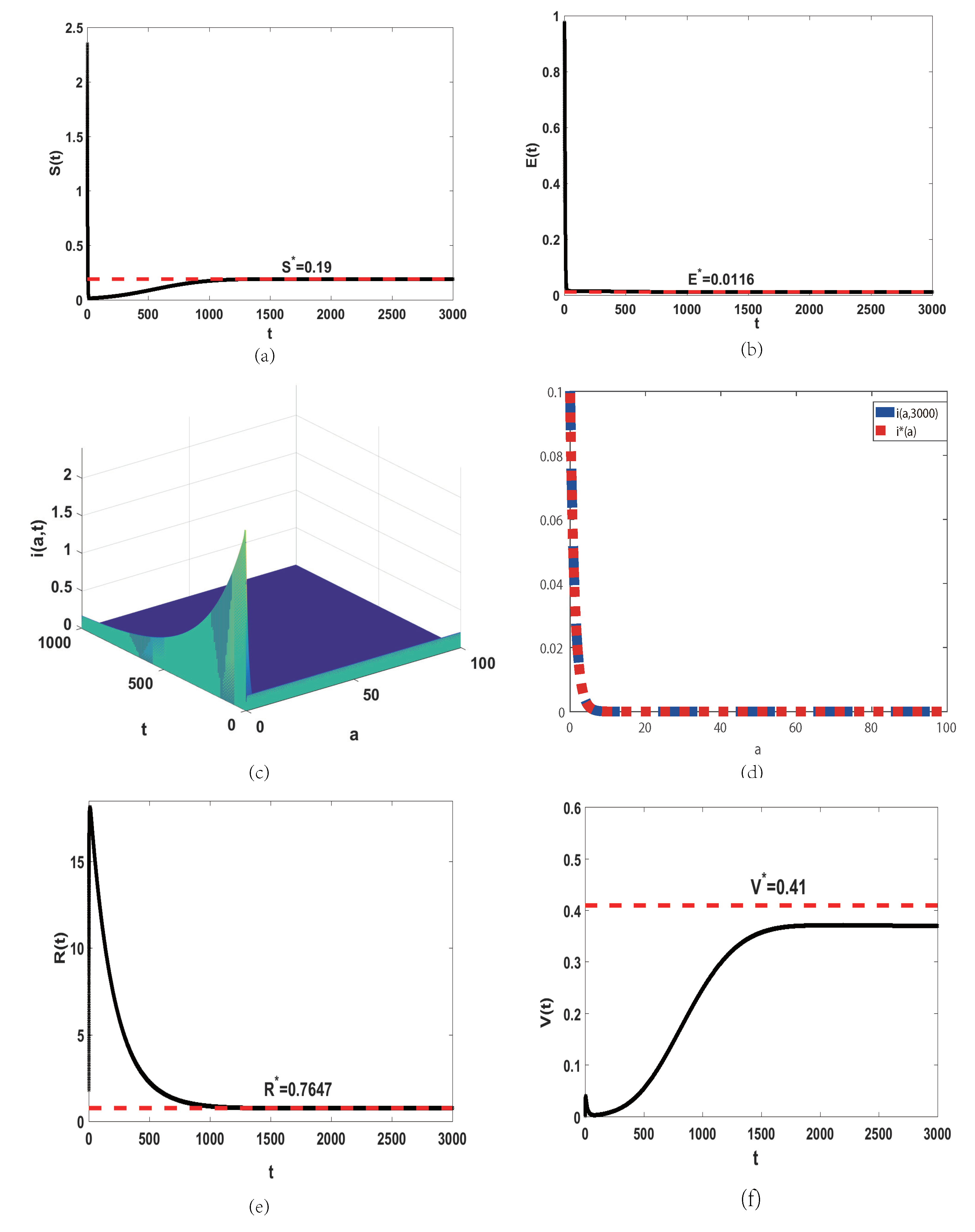
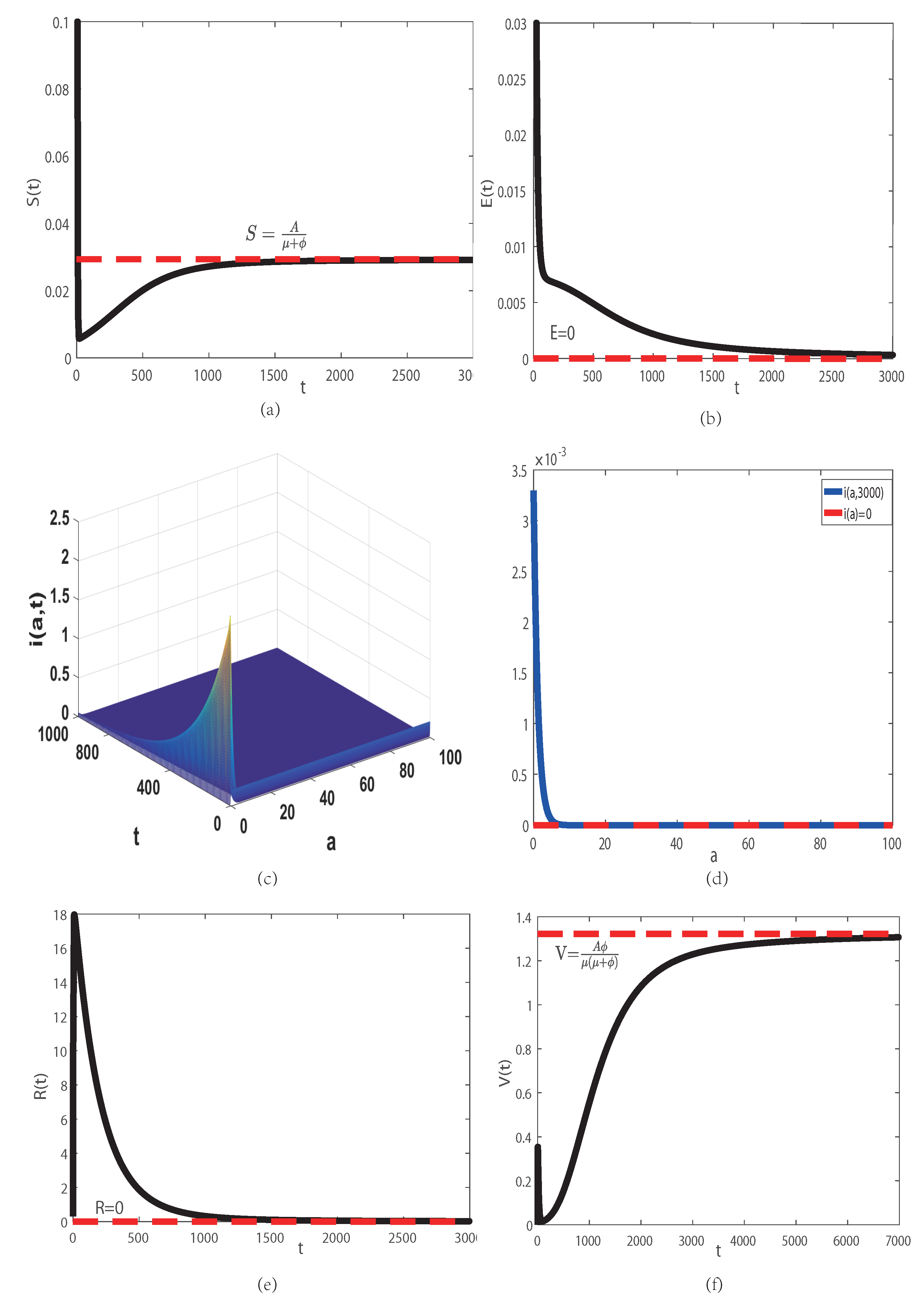
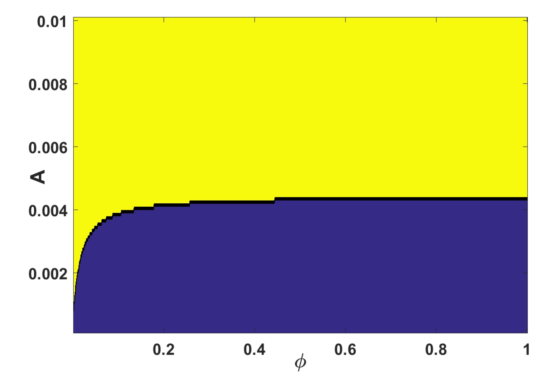
5. Numerical Simulations

In this section, we illustrate the theoretical results for system (3a–e)–(5) through numerical simulations. By the Euler Method, Theorems 5 and 6 hold true.

(i)

An example when ${\mathfrak{R}}_0>1$

In this section, we provide an example and numerical results to support our theoretical results. We set model (3a–e) with a saturation incidence rate of $f(S(t))=S(t)$ and $g(i(a,t))=i(a,t)$. Let $\mu =\frac{20}{9008},\delta =0.125,\gamma =0.8,\rho =0.022,\omega =0.4$, and $\sigma =0.15$. The initial condition is set as $(2.5,0.0002,0.2,0.2,0.3)$. We assume that the maximum age for the upper bound of infection age is 100 days, that people are more likely to be infected when $a\in (3,8]$, and that people will be cured or sent to the hospital for isolation and treated when $a>20$. So, the transmission coefficient $\beta (a)$ is chosen as

$$\beta (a)=\left\{\begin{array}{ccc}\hfill 0.15& \hfill & \hfill a\le 3,\\ \hfill 0.25& \hfill & \hfill 3<a\le 8,\\ \hfill 0.15& \hfill & \hfill 8<a\le 14,\\ \hfill 0.1& \hfill & \hfill 14<a\le 20,\\ \hfill 0& \hfill & \hfill a>20.\end{array}\right.$$

(77)

First, we set $A=0.006,\varphi =\frac{1}{100}$. By calculating Equations (27a–f), model (3a)–(5) has the disease-free equilibrium $E_1(0.49,2.21,0,0,0)$ and the endemic equilibrium $E_2$(0.19, 0.41, 0.0116, 0.1$e^{-0.82a}$, 0.7647). From Theorem 6, $E_2$ is globally asymptotically stable because ${\mathfrak{R}}_0>1$, as shown in Figure 1.

(ii)

An example when ${\mathfrak{R}}_0<1$

Next, let $A=0.003,\varphi =0.1$. Other parameters and initial conditions are the same as those in the above example. Model (3a–e)–(5) has only one disease-free equilibrium $E_1(\frac{A}{\mu +\varphi },\frac{A\varphi }{\mu (\mu +\varphi )},0,0,0)$, which is globally asymptotically stable because ${\mathfrak{R}}_0<1$, as shown in Figure 2.

(iii)

Effect of parameters A and $\varphi$ on ${\mathfrak{R}}_0$

As shown in Equation (34), the values of parameters A and $\varphi$ affect ${\mathfrak{R}}_0$. Will ${\mathfrak{R}}_0<1$ hold if $\varphi$ is large? From Figure 3, ${\mathfrak{R}}_0<1$ holds only when A is small and $\varphi$ is large. Clearly, ${\mathfrak{R}}_0<1$ cannot hold for large values of A.

6. Conclusions

In this paper, we investigated a SEIR model that considers age of infection and vaccination. Through an analysis, we obtained a basic reproduction number $\sqrt{{\mathfrak{R}}_0}$, which is the threshold of the dynamics of the model. The positivity, boundedness, and asymptotic smoothness of the solutions are shown. There exists only one disease-free equilibrium that is locally and globally asymptotically stable when ${\mathfrak{R}}_0<1$. There exists one unstable disease-free equilibrium and a unique locally stable endemic equilibrium for ${\mathfrak{R}}_0>1$. Furthermore, the endemic equilibrium is globally stable if functions $f(·)$ and $g(·)$ satisfy Assumption 3 and ${\mathfrak{R}}_0>1$.

According to our analysis, the recruitment rate of susceptible individuals A has an important effect on the spread of infectious diseases. Therefore, measures such as restrictions on travel and public gatherings should still be taken for a long time to keep the recruitment rate of susceptible individuals A low, even when we have vaccinations. Our work may be helpful in predicting and eliminating infectious diseases. It does not consider many factors, such as variations in parameters over time or control strategies; hence, our future work will consider the dynamic behaviors of models with parameters that vary with time and control strategies for eliminating the occurrence of infectious diseases.

References

1. Kermack, W.O.; McKendrick, A.G. A contribution to mathematical theory of epidemics. Proc. R. Soc. Lond. A 1927, 115, 700–721. [Google Scholar]
2. Kermack, W.O.; McKendrick, A.G. Contributions to the mathematical theory of epidemics II. The problem of endemicity. Bull. Math. Biol. 1991, 53, 57–87. [Google Scholar] [PubMed]
3. Kermack, W.O.; McKendrick, A.G. Contributions to the mathematical theory of epidemics III. Further studies of the problem of endemicity. Bull. Math. Biol. 1991, 53, 89–118. [Google Scholar] [PubMed]
4. Inaba, H. Endemic threshold analysis for the Kermack-McKendrick reinfection model. J. Math. Monograph. 2016, 9, 105–133. [Google Scholar]
5. Wang, X.; Chen, Y.; Martcheva, M.; Rong, L. Asymptotic analysis of a vector-borne disease model with the age of infection. J. Biol. Dyn. 2020, 14, 332–367. [Google Scholar] [CrossRef] [PubMed] [Green Version]
6. Perasso, A.; Richard, Q. Implication of age-structrue on the dynamics of Lotka Volterra equations. Differ. Integral Equ. 2019, 32, 91–120. [Google Scholar]
7. Rost, G.; Wu, J. SEIR epidemiological model with varying infectivity and infinite delay. Math. Biosci. Eng. 2008, 5, 389–402. [Google Scholar] [PubMed]
8. Magal, P.; McCluskey, C.C.; Webb, G.G. Lyapunov functional and global asymptotic stability for an infection-age model. Appl. Anal. 2010, 89, 1109–1140. [Google Scholar] [CrossRef]
9. Inaba, H. Age-Structured Population Dynamics in Demography and Epidemiology; Springer: Singapore, 2017. [Google Scholar]
10. Okuwa, K.; Inaba, H.; Kuniya, T. Mathematical analysis for an age-structured SIRS epidemic model. Math. Biosci. Eng. 2019, 16, 6071–6102. [Google Scholar] [CrossRef] [PubMed]
11. Sigdel, R.P.; McCluskey, C.C. Global stability for an SEI model of infectious disease with immigration. Appl. Math. Comput. 2014, 243, 684–689. [Google Scholar] [CrossRef]
12. Kang, H.; Ruan, S.; Yu, X. Age-structured population dynamics with nonlocal diffusion. J. Dyn. Diff. Equ. 2020. [Google Scholar] [CrossRef]
13. Zhang, R.; Li, D.; Liu, S. Global analysis of an age-structured SEIR model with immigration of population and nonlinear incidence rate. J. Appl. Comput. 2019, 9, 1470–1492. [Google Scholar] [CrossRef]
14. Lin, J.; Xu, R.; Tian, X. Global dynamics of an age-structured cholera model with multiple transmissions, saturation incidence and imperfect vaccination. J. Biol. Dyn. 2019, 13, 69–102. [Google Scholar] [CrossRef] [Green Version]
15. Barril, C.; Calsina, A.; Cuadrado, S.; Ripoll, J. Reproduction number for an age of infection structured model. Math. Model. Nat. Phenom. 2021, 16, 42. [Google Scholar] [CrossRef]
16. Ahmed, H.M.; Elbarkouky, R.A.; Omar, O.A.M.; Ragusa, M.A. Models for COVID-19 daily confirmed cases in different countries. Mathematics 2021, 9, 659. [Google Scholar] [CrossRef]
17. Khan, M.A.; Ismail, M.; Ullah, S.; Farhan, M. Fractional order SIR model with generalized incidence rate. AIMS Math. 2020, 5, 1856–1880. [Google Scholar] [CrossRef]
18. Ríos-Gutiérrez, A.; Torres, S.; Arunachalam, V. Studies on the basic reproduction number in stochastic epidemic models with random perturbations. Adv. Differ. Equ. 2021, 2021, 288. [Google Scholar] [CrossRef]
19. Calsina, A.; Ripoll, J. Hopf bifurcation in a structured population model for the sexual phase of monogonont rotifers. J. Math. Biol. 2002, 45, 22–36. [Google Scholar] [CrossRef]
20. Posny, R.; Wang, J.; Mukandavire, Z.; Modnak, C. Analyzing transmission dynamics of cholera with public health interventions. Math. Biosci. 2015, 264, 38–53. [Google Scholar] [CrossRef]
21. Webb, G.F. Theory of Nonlinear Age-Dependent Population Dynamics; Marcel Dekker: New York, NY, USA, 1985. [Google Scholar]
22. Smith, H.L.; Thieme, H.R. Dynamical Systems and Population Persistence; Amecican Mathematical Society: Providence, RI, USA, 2011. [Google Scholar]
23. Barril, C.; Calsina, A.; Cuadrado, S.; Ripoll, J. On the basic reproduction number in continuously structured populations. Math. Meth. Appl. Sci. 2021, 44, 799–812. [Google Scholar] [CrossRef]
24. Breda, D.; Florian, F.; Ripoll, J.; Vermiglio, R. Efficient numerical computation of the basic reproduction number for structured populations. J. Comput. Appl. Math. 2021, 384, 113165. [Google Scholar] [CrossRef] [PubMed]
25. Barril, C.; Calsina, A.; Ripoll, J. A practical approach to R0 in continuous-time ecological models. Math. Methods Appl. Sci. 2017, 41, 8432–8445. [Google Scholar] [CrossRef]
Figure 1. The red dashed lines display the estimate of the endemic steady state E 2 ( 0.19 , 0.41 , 0.0116 , 0.1 e 0.82 a , 0.7647 ) of model (3a–e)–(5), while other color lines show solutions with initial conditions ( 2.5 , 0.0002 , 0.2 , 0.2 , 0.3 ) and parameters A = 0.006 , μ = 20 9008 , ϕ = 1 100 , δ = 0.125 , γ = 0.8 , ρ = 0.022 , ω = 0.4 , σ = 0.15 from the direct simulation. The values of S ( t ) , E ( t ) , R ( t ) , V ( t ) with respect to t are shown in (a,b,e,f), respectively. i ( a , t ) with respect of a and t is shown in (c). The value of i ( a , t ) with respect to a at t = 3000 is shown in (d).
Mathematics 09 02195 g001
Figure 2. The red dashed lines display the estimate of the disease-free equilibrium E 1 ( A μ + ϕ , A ϕ μ ( μ + ϕ ) , 0 , 0 , 0 ) of model (3a–e)–(5), while other color lines lines show solutions with A = 0.003 , ϕ = 0.1 from the direct simulation. The initial conditions and other parameters are the same as those in Figure 1. Similar to Figure 1, (a) S ( t ) , (b) E ( t ) , (e) R ( t ) and (f) V ( t ) with respect to t are shown. (c) i ( a , t ) with respect to a and t is displayed. (d) i ( a , t ) with respect to a at t = 3000 is shown.
Mathematics 09 02195 g002
Figure 3. The yellow area corresponds to R 0 > 1 , while the blue area is R 0 < 1 of model (3a–e)–(5) with the same initial conditions and parameters as those in Figure 1.
Mathematics 09 02195 g003
Publisher’s Note: MDPI stays neutral with regard to jurisdictional claims in published maps and institutional affiliations.