Principal Component Analysis and Factor Analysis for an Atanassov IF Data Set

Abstract

The present contribution is devoted to the theory of fuzzy sets, especially Atanassov Intuitionistic Fuzzy sets (IF sets) and their use in practice. We define the correlation between IF sets and the correlation coefficient, and we bring a new perspective to solving the problem of data file reduction in case sets where the input data come from IF sets. We present specific applications of the two best-known methods, the Principal Component Analysis and Factor Analysis, used to solve the problem of reducing the size of a data file. We examine input data from IF sets from three perspectives: through membership function, non-membership function and hesitation margin. This examination better reflects the character of the input data and also better captures and preserves the information that the input data carries. In the article, we also present and solve a specific example from practice where we show the behavior of these methods on data from IF sets. The example is solved using R programming language, which is useful for statistical analysis of data and their graphical representation.

1. Introduction

In mathematics, just as in other scientific disciplines, there is a shift from theoretical mathematics to mathematics which would be applicable in practice. Such mathematics knowledge includes the field of statistics and probability. The theory of probability is a relatively young mathematical discipline whose axiomatic construction was built by Russian mathematician Kolmogorov in 1933 [1]. For the first time in history, the basic concepts of probability theory were defined precisely but simply. A random event was defined as a subset of a space, a random variable as a measurable function, and its mean value as an integral (abstract Lebesgue integral). Like the Kolmogorov theory of probability in the first half of the 20th century, the Zadeh fuzzy set played an important role in the second half of the 20th century [2,3,4,5]. Zadeh’s concept of a fuzzy set was generalized by Atanassov. In May 1983 it turned out that the new sets allow the definition of operators which are, in a sense, analogous to the modal ones (in the case of ordinary fuzzy sets such operators are meaningless, since they reduce to identity). It was then that the author realized that he had found a promising direction of research and published the results in [6]. Atanassov defined Intuitionistic Fuzzy sets (IF sets) and described them in terms of membership value, non-membership value and hesitation margin [7,8]. An IF set is a pair of functions $=\left({\mu }_A,{\nu }_A\right)$ where function ${\mu }_A:\mathsf{\Omega }\to \langle 0,1\rangle$ is called the membership function and function ${\nu }_A:\mathsf{\Omega }\to \langle 0,1\rangle$ is called the non-membership function, in force that ${\mu }_A+{\nu }_A\le 1$. Many writers have attempted to prove some known assertions from the classical probability theory in the theory of IF sets [9,10,11,12] and apply known statistical methods in these sets.

In 2010, Bujnowski P., Kacprzyk J., and Szmidt E. [13] defined a correlation coefficient (more in Section 3) and presented novel-approach dimensionality reduction data sets through Principal Component Analysis on IF sets [14]. For this article, we saw the practical use of IF sets to solve the problem of the reduction of dimensionality data sets. Therefore, it motivated us to continue this idea.

One of the main problems in data analysis is to reduce the number of variables while maintaining the maximum information that the data carries. Among the most-used methods to reduce the dimension of data are Principal Component Analysis (PCA) and Factor Analysis (FA) (more in Section 2). The source data from an IF set accurately reflect the nature of the component under investigation. In the classical case of the use of methods PCA and FA, we examine the sample only from a one-sided view. In the case of data from an IF set, the sample is examined from two views: membership function and non-membership function. Alternatively, we can talk about up to three views if we include the degree of uncertainty of the IF set of a given data sample. The degree of uncertainty can be defined for each IF set in $\mathsf{\Omega }$ by the formula

$${\pi }_A\left(\omega \right)=1-{\mu }_A\left(\omega \right)-{\nu }_A\left(\omega \right)$$

(1.1)

while $0\le {\pi }_A\left(\omega \right)\le 1$ for each $\omega \in \mathsf{\Omega }$ [15].

Based on the above, an IF set better describes the character of the studied compounds. The paper aims to show the use of data from an IF set to address a specific example for known methods used to reduce the dimensions of the data set. The comparison of methods with classical theory and the comparison of methods with each other are used to reduce the dimensions of the data set. The rest of the paper is organized as follows: Section 2 contains the methods’ description. Section 3 defines the correlation between IF sets. Section 4 contains the specific example of the use of Principal Component Analysis and Factor Analysis methods. Section 5 contains the conclusion, a comparison of methods and a discussion.

2. Methods’ Description

Principal Component Analysis (PCA) was introduced in 1901 by Karl Pearson [16]. The method aims to transform the input multi-dimensional data so that the output data of the most important linear directions is obtained, with the least significant directions being ignored. Thus, we extract the characteristic directions (characters) from the original data and at the same time reduce the data dimension. The method is one of the basic methods of data compression—original $n$ variables can be represented by a smaller number $m$ of variables while explaining a sufficiently large part of the variability of the original data set. The system of new variables (the so-called main components) consists of a linear combination of the original variables. The first main component describes the largest part of the variability of the original data set. The other major components contribute to the overall variance, always with a smaller proportion. All pairs of main components are perpendicular to each other [17]).

The basic steps of the PCA include the construction of a correlation matrix from source data, the calculation of eigenvalues of the correlation matrix, the alignment from the largest $\left({\lambda }_1>\cdots >{\lambda }_n\right)$, the calculation of eigenvectors of the correlation matrix corresponding to its eigenvalues $\left({\upsilon }_1,\dots ,{\upsilon }_n\right)$, the calculation of the variability of the original data $\left({\sigma }^2\right)$, the determination of the number of main components sufficient to represent the original variables based on variability and the transfer of the original data to a new base. The number of major components (MC) is determined either by our consideration of the need to maintain information (eigenvalues, which explain e.g., 90% of variability). By Kaiser’s Rule using those MC whose eigenvalue is greater than the average of all eigenvalues (with standard data, the average is 1, i.e., taking the MC, whose eigenvalue is greater than 1), we use MC, which together account for at least 70% of the total variance, or based on a graphical display, the so-called Screen Plot chart, where we find a turning point in this chart and take MC into account for this turning point.

Factor Analysis (FA) was introduced in 1904 by Charles Edward Spearman and described in 1995 by Bartholomew D. J. [18]. This method allows new variables to be created from a set of original variables. It allows you to find hidden (latent) causes that are a source of data variability. With latent variables, it is possible to reduce the number of variables while keeping the maximum amount of information, and to establish a link between observable causes and new variables (factors). If we assume that input variables are correlated, then the same amount of information can be described by fewer variables. In the resulting solution, each original variable should be correlated with as few factors as possible, and the number of factors should be minimal. The factor saturations reflect the influence of the $k$th common factor on the $j$th random variable. Several methods are used to estimate factor saturation, so-called factor extraction methods. In our paper, we used the method of the main components. Other known methods include the maximum plausibility method or the least-squares method.

The number of common factors can be determined either by the eigenvalue criterion (the so-called Kaiser’s Rule), when factors which have their eigenvalues $\lambda >1$ are considered significant. The reliability of this rule depends on the number of input variables (if the number of variables is between 20 and 50, the rule is reliable, if the number is less than 20, there is an erroneous tendency to determine a smaller number of factors, and if the number is greater than 50, this leads to a false determination of a large number of factors) and the criterion of the percentage of explained variability when common factors should explain as much as possible the total variability. Alternatively, it depends on the Screen Plot chart of eigenvalues (it is recommended that several factors be used; they are located in front of the turning point on the chart). The basic steps of FA are the selection of input data (assumption of correlation), the determination of the common factors, the estimation of parameters (if the communality is less than 0.5, it is appropriate to exclude the given indicator from the analysis), the rotation of factors (Varimax Method—orthogonal rotation) and the factor matrix (factor saturation matrix). High factor saturation means that the factor significantly influences the indicator. Those factors whose absolute value is greater than 0.3 are considered to be statistically significant, medium significant factors are those with an absolute value greater than 0.4, and very significant factors are those with an absolute value greater than 0.5 [17]. The main idea of the methods is to reduce the number of variables (reduce the dimension of the data file) while maintaining the highest variability of the original data. For both methods we need the construction of a correlation matrix from source data. Therefore, we need to define the correlation coefficient for IF sets.

3. Correlation between IF Sets

The correlation between IF sets was introduced by Szmidt and Kacprzyk in 2010 [13]. Let $A,B$ are IF sets be defined at $\mathsf{\Omega }=\left\{{\omega }_1,{\omega }_2,\dots ,{\omega }_n\right\}$. Sets $A,B$ are characterized by pair sequence:

$$\begin{gathered} \left[\left({\mu }_A\left({\omega }_1\right),{\nu }_A\left({\omega }_1\right),{\pi }_A\left({\omega }_1\right)\right),\left({\mu }_B\left({\omega }_1\right),{\nu }_B\left({\omega }_1\right),{\pi }_B\left({\omega }_1\right)\right)\right], \\ \left[\left({\mu }_A\left({\omega }_2\right),{\nu }_A\left({\omega }_2\right),{\pi }_A\left({\omega }_2\right)\right),\left({\mu }_B\left({\omega }_2\right),{\nu }_B\left({\omega }_2\right),{\pi }_B\left({\omega }_2\right)\right)\right], \\ \dots \\ \left[\left({\mu }_A\left({\omega }_n\right),{\nu }_A\left({\omega }_n\right),{\pi }_A\left({\omega }_n\right)\right),\left({\mu }_B\left({\omega }_n\right),{\nu }_B\left({\omega }_n\right),{\pi }_B\left({\omega }_n\right)\right)\right], \end{gathered}$$

where each function corresponds to the competence function, the incompetence function, and the degree of uncertainty of the sets $A$ and $B$.

Definition 1.

(Szmidt, Kacprzyk, Bujnowski [14]) The correlation coefficient $r_{A-IFS}\left(A,B\right)$ between two IF sets $A$ and $B$ in $\mathsf{\Omega }$ is:

$$r_{A-IFS}\left(A,B\right)=\frac{1}{3}\left(r_1\left(A,B\right)+r_2\left(A,B\right)+r_3\left(A,B\right)\right)$$

(1.2)

where

$$r_1\left(A,B\right)=\frac{{{\displaystyle \sum }}_{i=1}^n\left({\mu }_A\left({\omega }_i\right)-\overline{{\mu }_A}\right)\left({\mu }_B\left({\omega }_i\right)-\overline{{\mu }_B}\right)}{{\left({{\displaystyle \sum }}_{i=1}^n{\left({\mu }_A\left({\omega }_i\right)-\overline{{\mu }_A}\right)}^2\right)}^{\frac{1}{2}}{\left({{\displaystyle \sum }}_{i=1}^n{\left({\mu }_B\left({\omega }_i\right)-\overline{{\mu }_B}\right)}^2\right)}^{\frac{1}{2}}}$$

(1.3)

$$r_2\left(A,B\right)=\frac{{{\displaystyle \sum }}_{i=1}^n\left({\nu }_A\left({\omega }_i\right)-\overline{{\nu }_A}\right)\left({\nu }_B\left({\omega }_i\right)-\overline{{\nu }_B}\right)}{{\left({{\displaystyle \sum }}_{i=1}^n{\left({\nu }_A\left({\omega }_i\right)-\overline{{\nu }_A}\right)}^2\right)}^{\frac{1}{2}}{\left({{\displaystyle \sum }}_{i=1}^n{\left({\nu }_B\left({\omega }_i\right)-\overline{{\nu }_B}\right)}^2\right)}^{\frac{1}{2}}}$$

(1.4)

$$r_3\left(A,B\right)=\frac{{{\displaystyle \sum }}_{i=1}^n\left({\pi }_A\left({\omega }_i\right)-\overline{{\pi }_A}\right)\left({\pi }_B\left({\omega }_i\right)-\overline{{\pi }_B}\right)}{{\left({{\displaystyle \sum }}_{i=1}^n{\left({\pi }_A\left({\omega }_i\right)-\overline{{\pi }_A}\right)}^2\right)}^{\frac{1}{2}}{\left({{\displaystyle \sum }}_{i=1}^n{\left({\pi }_B\left({\omega }_i\right)-\overline{{\pi }_B}\right)}^2\right)}^{\frac{1}{2}}}$$

(1.5)

At the same time

$$\overline{{\mu }_A}=\frac{1}{n}{\displaystyle \sum }_{i=1}^n{\mu }_A\left({\omega }_i\right),\overline{{\nu }_A}=\frac{1}{n}{\displaystyle \sum }_{i=1}^n{\nu }_A\left({\omega }_i\right),\overline{{\pi }_A}=\frac{1}{n}{\displaystyle \sum }_{i=1}^n{\pi }_A\left({\omega }_i\right)$$

$$\overline{{\mu }_B}=\frac{1}{n}{\displaystyle \sum }_{i=1}^n{\mu }_B\left({\omega }_i\right),\overline{{\nu }_B}=\frac{1}{n}{\displaystyle \sum }_{i=1}^n{\nu }_B\left({\omega }_i\right),\overline{{\pi }_B}=\frac{1}{n}{\displaystyle \sum }_{i=1}^n{\pi }_B\left({\omega }_i\right)$$

The correlation coefficient (1.2) depends on the amount of information expressed as a competence function and as an incompetence function (1.3), (1.4) as well as the reliability of the information expressed as a degree of uncertainty (1.5). For the correlation coefficient (1.2), the following properties apply [14]:

• $r_{A-IFS}\left(A,B\right)=r_{A-IFS}\left(B,A\right)$
• If $A=B$, then $r_{A-IFS}\left(A,B\right)=1$
• $\left|r_{A-IFS}\left(A,B\right)\right|\le 1$

These properties apply to each element (1.3)—(1.5). The correlation coefficient $r_{A-IFS}\left(A,B\right)=1$ not only for $A=B$ but also for the perfect linear correlation of data [5].

4. Use of PCA and FA Methods

We have selected the 20 most sold car brands for 2020 (we tracked sales for a period of 12 months). The data come from our own survey, in which we asked car dealers in two cities (Nitra and Žilina, Slovak Republic) about the best-selling car brands in 2020. There were 20 brands listed and 5 criteria were assessed (the criteria were not specifically selected, they were created on the basis of most common questions that buyers ask when buying a car): A—power, B—equipment, C—price, D—driving properties, E—consumption. Each criterion was evaluated twice: the percentage the criterion is met for each participant and the percentage the criterion is not met. The results are in

Table 1. The competence and the incompetence functions.

	A (%)		B (%)		C (%)		D (%)		E (%)
Brand	m	nm	m	nm	m	nm	m	nm	m	nm
1	84	7	81	11	31	49	90	6	70	20
2	73	13	53	30	20	63	53	21	60	27
3	56	13	65	14	4	76	59	14	55	18
4	77	11	63	4	11	60	41	20	62	10
5	93	4	71	11	29	47	76	14	63	33
6	53	35	57	38	38	50	47	46	44	37
7	91	3	85	11	24	56	75	10	25	21
8	88	6	48	12	45	26	58	40	51	40
9	69	15	62	11	5	90	74	16	78	8
10	36	25	82	6	11	77	70	22	61	22
11	62	31	71	17	17	76	48	22	79	16
12	62	27	49	16	18	57	76	2	56	34
13	62	31	60	24	44	38	47	27	81	18
14	55	30	50	33	38	57	76	17	48	26
15	61	38	58	18	56	41	62	28	35	24
16	71	4	55	16	20	76	42	49	90	5
17	50	39	60	27	6	91	48	36	54	36
18	75	11	88	1	20	61	74	7	56	4
19	74	6	67	6	23	67	84	8	67	24
20	59	27	64	21	39	51	66	12	78	8

below.

Data A, B, C, D and E from Table 1 are assigned the competence and incompetence functions. Since the values in Table 1 are expressed as percentages, we can easily assign the competence function of the values in the “met” column and the incompetence function to the values in the “not met” column, provided $\mu ,\nu \in \langle 0,1\rangle$ that a $\mu +\nu \le 1$ for A, B, C, D, and E. Then these values are IF data. From the relationship (1.1) we calculate the degree of uncertainty for A, B, C, D, and E (

Table 2. Degree of uncertainty.

	A			B			C			D			E
Brand	${\mathit{\mu }}_{\mathit{A}}$	${\mathit{\nu }}_{\mathit{A}}$	${\mathit{\pi }}_{\mathit{A}}$	${\mathit{\mu }}_{\mathit{B}}$	${\mathit{\nu }}_{\mathit{B}}$	${\mathit{\pi }}_{\mathit{B}}$	${\mathit{\mu }}_{\mathit{C}}$	${\mathit{\nu }}_{\mathit{C}}$	${\mathit{\pi }}_{\mathit{C}}$	${\mathit{\mu }}_{\mathit{D}}$	${\mathit{\nu }}_{\mathit{D}}$	${\mathit{\pi }}_{\mathit{D}}$	${\mathit{\mu }}_{\mathit{E}}$	${\mathit{\nu }}_{\mathit{E}}$	${\mathit{\pi }}_{\mathit{E}}$
1	0.84	0.07	0.09	0.81	0.11	0.08	0.31	0.49	0.20	0.90	0.06	0.04	0.70	0.20	0.10
2	0.73	0.13	0.14	0.53	0.30	0.17	0.20	0.63	0.17	0.53	0.21	0.26	0.60	0.27	0.13
3	0.56	0.13	0.31	0.65	0.14	0.21	0.04	0.76	0.20	0.59	0.14	0.27	0.55	0.18	0.27
4	0.77	0.11	0.12	0.63	0.04	0.33	0.11	0.60	0.29	0.41	0.20	0.39	0.62	0.10	0.28
5	0.93	0.04	0.03	0.71	0.11	0.18	0.29	0.47	0.24	0.76	0.14	0.10	0.63	0.33	0.04
6	0.53	0.35	0.12	0.57	0.38	0.05	0.38	0.50	0.12	0.47	0.46	0.07	0.44	0.37	0.19
7	0.91	0.03	0.06	0.85	0.11	0.04	0.24	0.56	0.20	0.75	0.10	0.15	0.25	0.21	0.54
8	0.88	0.06	0.06	0.48	0.12	0.40	0.45	0.26	0.29	0.58	0.40	0.02	0.51	0.40	0.09
9	0.69	0.15	0.16	0.62	0.11	0.27	0.05	0.90	0.05	0.74	0.16	0.10	0.78	0.08	0.14
10	0.36	0.25	0.39	0.82	0.06	0.12	0.11	0.77	0.12	0.70	0.22	0.08	0.61	0.22	0.17
11	0.62	0.31	0.07	0.71	0.17	0.12	0.17	0.76	0.07	0.48	0.22	0.30	0.79	0.16	0.05
12	0.62	0.27	0.11	0.49	0.16	0.35	0.18	0.57	0.25	0.76	0.02	0.22	0.56	0.34	0.10
13	0.62	0.31	0.07	0.60	0.24	0.16	0.44	0.38	0.18	0.47	0.27	0.26	0.81	0.18	0.01
14	0.55	0.30	0.15	0.50	0.33	0.17	0.38	0.57	0.05	0.76	0.17	0.07	0.48	0.26	0.26
15	0.61	0.38	0.01	0.58	0.18	0.24	0.56	0.41	0.03	0.62	0.28	0.10	0.35	0.24	0.41
16	0.71	0.04	0.25	0.55	0.16	0.29	0.20	0.76	0.04	0.42	0.49	0.09	0.90	0.05	0.05
17	0.50	0.39	0.11	0.60	0.27	0.13	0.06	0.91	0.03	0.48	0.36	0.16	0.54	0.36	0.10
18	0.75	0.11	0.14	0.88	0.01	0.11	0.20	0.61	0.19	0.74	0.07	0.19	0.56	0.04	0.40
19	0.74	0.06	0.20	0.67	0.06	0.27	0.23	0.67	0.10	0.84	0.08	0.08	0.67	0.24	0.09
20	0.59	0.27	0.14	0.64	0.21	0.15	0.39	0.51	0.10	0.66	0.12	0.22	0.78	0.08	0.14

).

First, we will conduct the Principal Component Analysis. We start by calculating the values of the correlation matrices from the values of the input variables of the competence function $R_{\mu }$, the incompetence function $R_{\nu }$ and the degree of uncertainty $R_{\pi }$. We calculate the values of the correlation matrices from Equations (1.3)–(1.5).

$$R_{\mu }=\left(\begin{array}{ccccc}1.00000000& 0.17614030& 0.15817266& 0.26372330& -0.06097966\\ 0.17614030& 1.00000000& -0.25863849& 0.41187539& -0.05797482\\ 0.15817266& -0.25863849& 1.00000000& 0.05248103& -0.22512182\\ 0.26372330& 0.41187539& 0.05248103& 1.00000000& -0.18133075\\ -0.06097966& -0.05797482& -0.22512182& -0.18133075& 1.00000000\end{array}\right)$$

$$R_{\mu }=\left(\begin{array}{ccccc}1.00000000& 0.17614030& 0.15817266& 0.26372330& -0.06097966\\ 0.17614030& 1.00000000& -0.25863849& 0.41187539& -0.05797482\\ 0.15817266& -0.25863849& 1.00000000& 0.05248103& -0.22512182\\ 0.26372330& 0.41187539& 0.05248103& 1.00000000& -0.18133075\\ -0.06097966& -0.05797482& -0.22512182& -0.18133075& 1.00000000\end{array}\right)$$

$$R_{\nu }=\left(\begin{array}{ccccc}1.0000000& 0.61169656& 0.06464770& 0.25152916& 0.2390998\\ 0.6116966& 1.00000000& -0.09219544& 0.45217323& 0.4269612\\ 0.0646477& -0.09219544& 1.00000000& -0.03038455& -0.3267094\\ 0.2515292& 0.45217323& -0.03038455& 1.00000000& 0.2221003\\ 0.2390998& 0.42696123& -0.32670936& 0.22210033& 1.0000000\end{array}\right)$$

$$R_{\pi }=\left(\begin{array}{ccccc}1.00000000& 0.01429969& -0.18037422& -0.02824073& -0.06232790\\ 0.01429969& 1.00000000& 0.25376953& 0.04773643& -0.25863891\\ -0.18037422& 0.25376953& 1.00000000& 0.26175490& 0.04768127\\ -0.02824073& 0.04773643& 0.26175490& 1.00000000& 0.06177976\\ -0.06232790& -0.25863891& 0.04768127& 0.06177976& 1.00000000\end{array}\right)$$

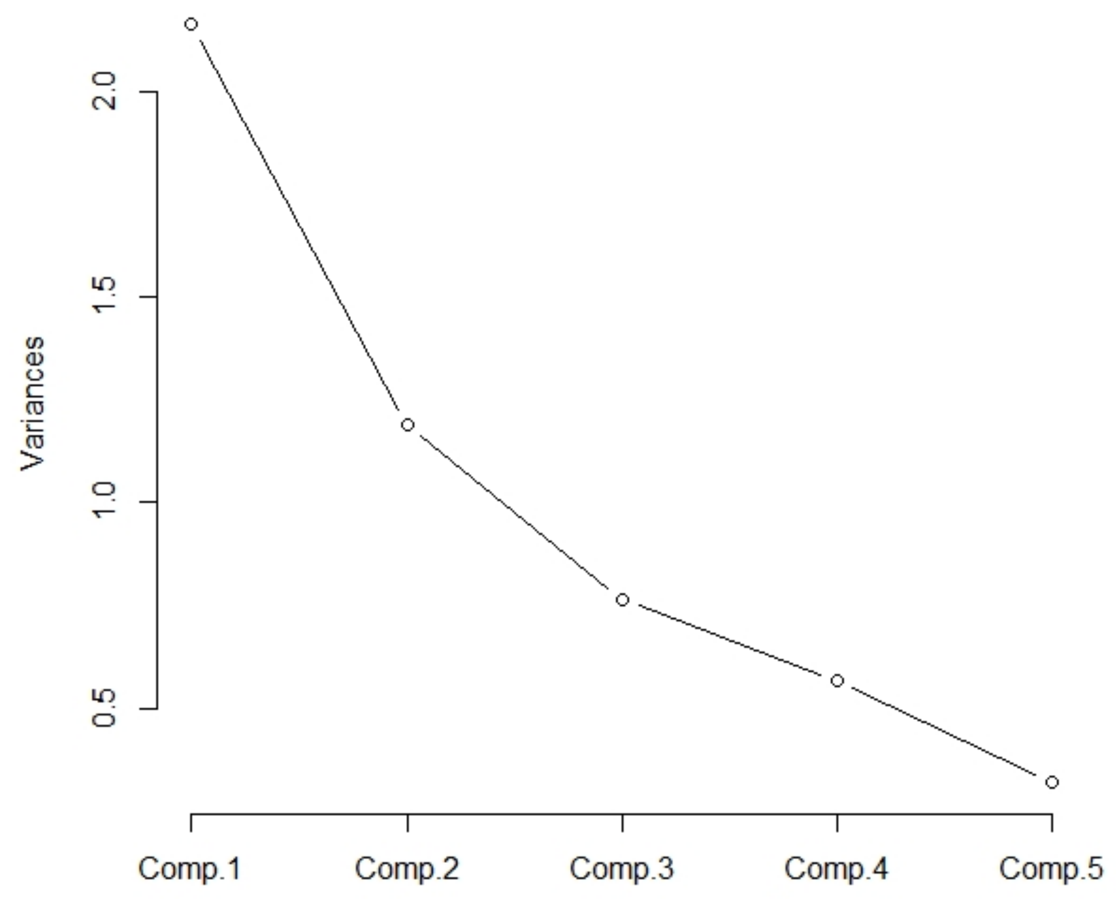
The eigenvalues of the correlation matrix $R_{\mu }$ are: ${\lambda }_1=$ 1.6328865, ${\lambda }_2=$ 1.3278224, ${\lambda }_3=$ 0.9150624, ${\lambda }_4=$ 0.6406398, ${\lambda }_5=$ 0.4835889. The variability of the input variables (sum of the elements on the main diagonal = sum of the eigenvalues of the correlation matrix) is ${\sigma }^2=$ 5. The eigenvalues are displayed on the charts (Figure 1,

Table 3. The PCA results calculated using the R program are as follows.

Importance of Components:
	Comp.1	Comp.2	Comp.3	Comp.4	Comp.5
Standard deviation	1.2778445	1.1523118	0.9565889	0.8003998	0.69540557
Proportion of Variance	0.3265773	0.2655645	0.1830125	0.1281280	0.09671778
Cumulative Proportion	0.3265773	0.5921418	0.7751543	0.9032822	1.00000000

). From the graph, we can see that the turning point is behind the third component. Additionally, according to Kaiser’s Rule, the first two components are considered.

In the row “Standard deviation”, there are the values of the main components, hence $\left(\sqrt{{\lambda }_i},i=1,2,3,4,5\right)$. In the row “Proportions of Variance”, there are the shares of variability $\frac{{\lambda }_i}{{\sigma }^2},i=1,2,3,4,5$. And in the row “Cumulative Proportion”, there are the cumulative shares of variability. We can see that the first two components meet 77.52% of the input data variability.

We will do the same for the values of the incompetence function input variables and the degree of uncertainty.

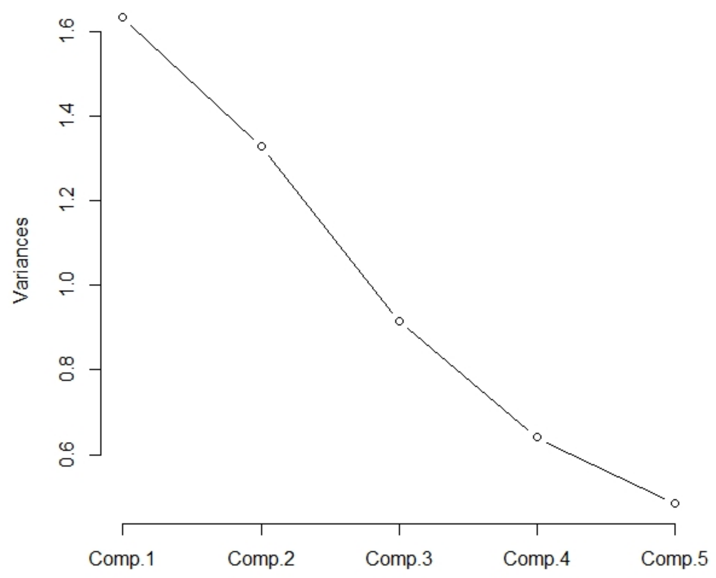
The eigenvalues of the correlation matrix $R_{\nu }$ are ${\lambda }_1=$ 2.1645080, ${\lambda }_2=$ 1.1884539, ${\lambda }_3=$ 0.7637763, ${\lambda }_4=$ 0.5663754, ${\lambda }_5=$ 0.3168864. The variability of the input variables is ${\sigma }^2=5$. The eigenvalues are displayed on the charts (Figure 2,

Table 4. The PCA results calculated using the R program are as follows.

Importance of Components:
	Comp.1	Comp.2	Comp.3	Comp.4	Comp.5
Standard deviation	1.4712267	1.0901623	0.8739429	0.7525792	0.56292667
Proportion of Variance	0.4329016	0.2376908	0.1527553	0.1132751	0.06337729
Cumulative Proportion	0.4329016	0.6705924	0.8233476	0.9366227	1.00000000

). According to the graph, the turning point could be located after the second component. Both the first two components are considered from the graph and the Kaiser Rule.

The first two components meet 67.06% of the input data variability, which is insufficient. The first three components meet 82.33% of the input data variability, which is permissible.

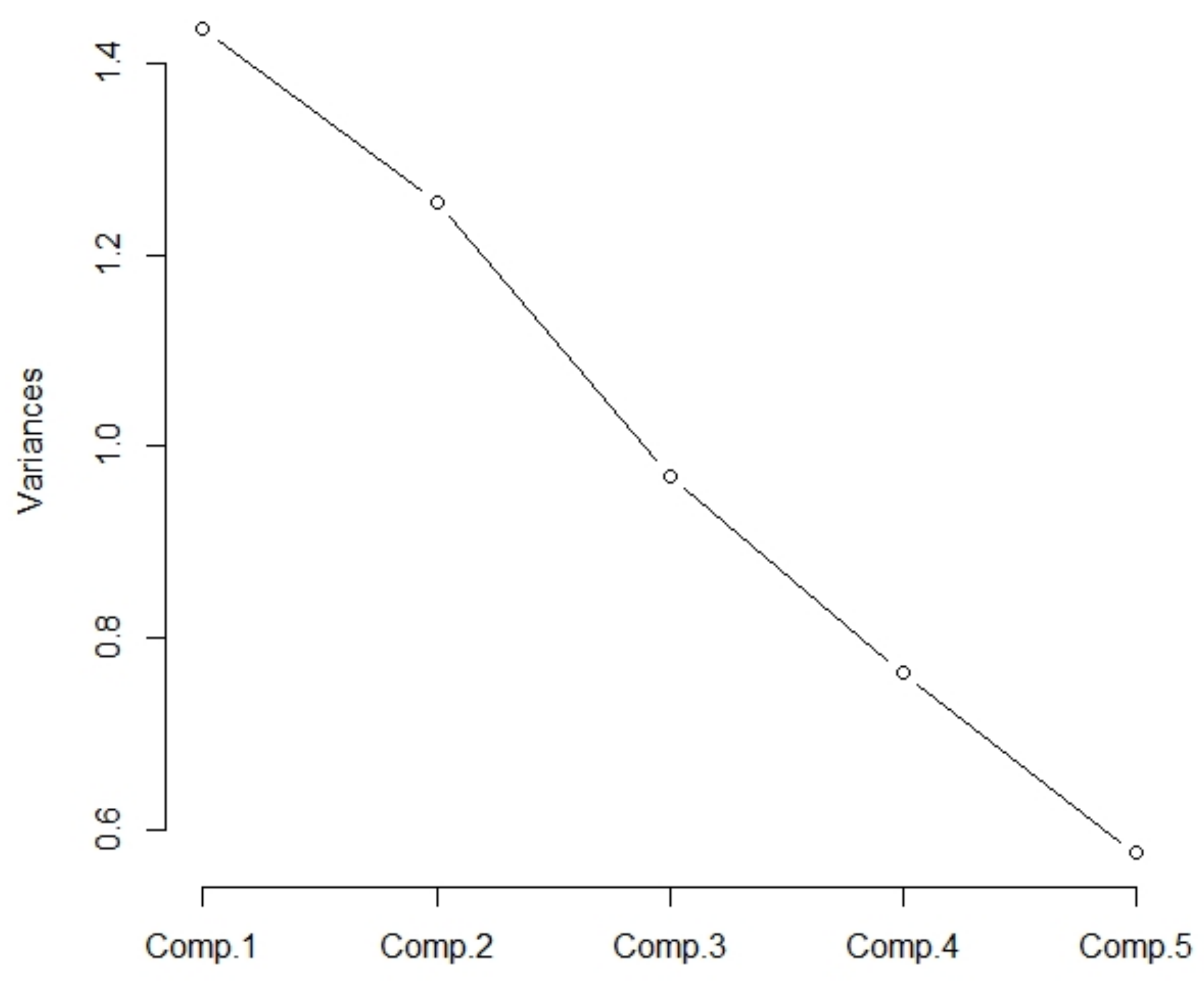
The eigenvalues of the correlation matrix $R_{\pi }$ are ${\lambda }_1=$ 1.4352248, ${\lambda }_2=$ 1.2553099, ${\lambda }_3=$ 0.9695103, ${\lambda }_4=$ 0.7644114, ${\lambda }_5=$ 0.5755435. The variability of the input variables is ${\sigma }^2=5$. The eigenvalues are displayed on the charts (Figure 3,

Table 5. The PCA results calculated using the R program are as follows.

Importance of Components:
	Comp.1	Comp.2	Comp.3	Comp.4	Comp.5
Standard deviation	1.198009	1.1204061	0.9846371	0.8743063	0.7586459
Proportion of Variance	0.287045	0.2510620	0.1939021	0.1528823	0.1151087
Cumulative Proportion	0.287045	0.5381069	0.7320090	0.8848913	1.0000000

). The turning point would be located behind the second component according to the graph. According to Kaiser’s Rule, the first two components are considered.

The first two components meet 53.81% of the input data variability, which is insufficient. The first three components meet 73.2% of the input data variability, which is permissible.

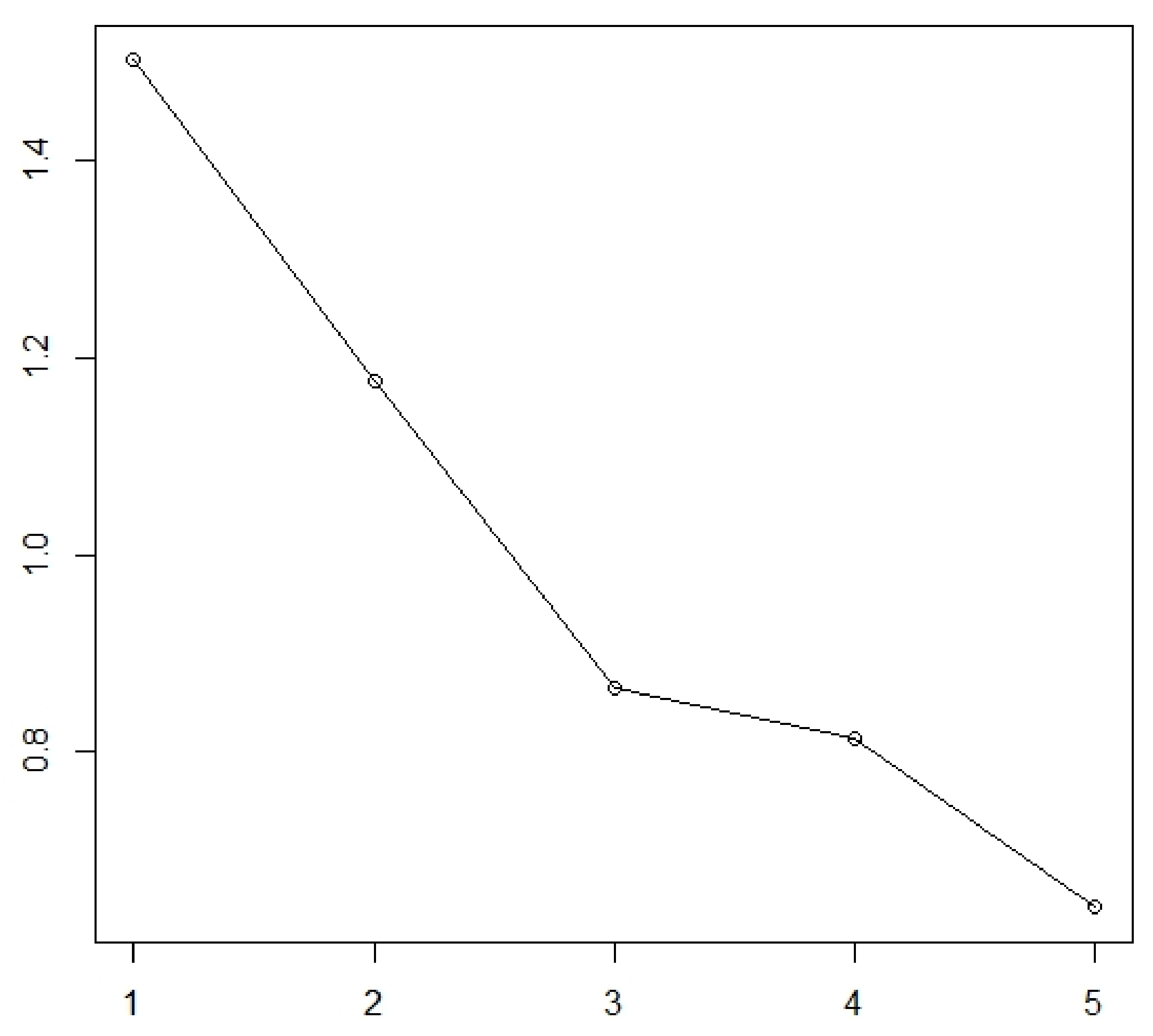
Now we calculate the correlation matrix R for the complete correlation of components according to (1.2).

$$R=\left(\begin{array}{ccccc}1.00000000& 0.2673789& 0.01414871& 0.16233724& 0.03859740\\ 0.2673789& 1.0000000& -0.03235480& 0.30392835& 0.03678250\\ 0.01414871& -0.0323548& 1.00000000& 0.09461713& -0.16804997\\ 0.16233724& 0.3039284& 0.09461713& 1.00000000& 0.03418311\\ 0.03859740& 0.0367825& -0.16804997& 0.03418311& 1.00000000\end{array}\right)$$

The eigenvalues of the correlation matrix R are ${\lambda }_1=$ 1.5023867, ${\lambda }_2=$ 1.1774258, ${\lambda }_3=$ 0.8652105, ${\lambda }_4=$ 0.8134299, ${\lambda }_5=$ 0.6415472. We will display them on the chart (Figure 4).

From the graph, it is visible that the turning point is located behind the third component. According to Kaiser’s Rule, the first two components which are considered meet 53.6% of the input data variability, which is insufficient. Therefore, we will consider the first three components that meet the 70.9% of input data variability, which is sufficient.

From the results received so far, we can determine the number of main components at 3. The results of the overall correlation also enable a reduction in the dimension from five to three, i.e., the original 5 components can be replaced by three main components while maintaining 70.9% of the original data variability.

We mark the eigenvectors of the covariance matrix $R_{\mu }$ as $V_{{\mu }_i},i=1,2,3,4,5$. Similarly, we mark our eigenvector of the covariance matrix $R_{\nu }$ as $V_{{\nu }_i}$ and the eigenvectors of the covariance matrix $R_{\pi }$ $V_{{\pi }_i}$ for $i=1,2,3,4,5$. The results of PCA are summarized in

Table 6. PCA results.

	${\mathit{V}}_{{\mathit{\mu }}_{\mathbf{1}}}$	${\mathit{V}}_{{\mathit{\mu }}_{\mathbf{2}}}$	${\mathit{V}}_{{\mathit{\mu }}_{\mathbf{3}}}$	${\mathit{V}}_{{\mathit{\nu }}_{\mathbf{1}}}$	${\mathit{V}}_{{\mathit{\nu }}_{\mathbf{2}}}$	${\mathit{V}}_{{\mathit{\nu }}_{\mathbf{3}}}$	${\mathit{V}}_{{\mathit{\pi }}_{\mathbf{1}}}$	${\mathit{V}}_{{\mathit{\pi }}_{\mathbf{2}}}$	${\mathit{V}}_{{\mathit{\pi }}_{\mathbf{3}}}$
A	−0.46	−0.19	0.69	0.49	−0.36	0.48	−0.27	0.35	0.81
B	−0.55	0.44	−0,14	0.60	−0,14	0.10	0.50	0.51	−0.04
C	−0.08	−0.75	0.16	−0.16	−0,80	0.02	0.67	−0.17	−0.01
D	−0.63	0.03	−0.06	0.43	−0.15	−0.85	0.46	−0.29	0.57
E	0.29	0.45	0.69	0.44	0.44	0.16	−0.12	−0.71	0.14

. The columns in the table represent the first three eigenvectors of the covariance matrices $R_{\mu }$, $R_{\nu }$, $R_{\pi }$. The main components are obtained by multiplying the eigenvectors with the original data.

In this way, we will gain a reduction in the dimension of the original data from five to three.

We will also address the cases of Factor Analysis based on the PCA method. Input data are shown in Table 2. The correlation matrices and their eigenvalues are calculated in the previous instance of the PCA method. As the number of input variables is 20, we are offered at least two criteria to determine the number of factors. The eigenvalue criterion determines for us two important factors (we can see this with eigenvalues of the correlation matrices $R_{\mu }$, $R_{\nu }$, $R_{\pi }$; only the first two values are greater than 1 in any case).

From the chart of eigenvalues, Figure 1, we can see that the turning point is behind the third component. From the graphs Figure 2 and Figure 3, we can see that the turning point is at the second component in both cases. Let us have a look at the variability of the data. If two factors are considered, data variability is very low in all cases. At three components, data variability is greater than 70%, so it is sufficient. Hence, we will further consider three factors. We will first solve the case of Factor Analysis (hereinafter FA) for the input data of the competence functions ${\mu }_A,{\mu }_B,{\mu }_C,{\mu }_D,{\mu }_E$. The first three factors represent 77.52% of the input data variability. We perform the FA using the R program (

Table 7. Factor Analysis.

Standardized Loadings (Pattern Matrix) Based upon Correlation Matrix
	RC1	RC2	RC3	h2
A	0.22	0.08	0.87	0.82
B	0.87	0.04	0.02	0.76
C	−0.46	−0.52	0.54	0.77
D	0.68	−0.28	0.34	0.66
E	−0.14	0.91	0.06	0.86

), and we use the Varimax method to rotate the factors.

At the output, we have a calculated matrix of factor saturation after rotations (columns RC1-RC3). In column h2, there are values of the communalities. We can see that the first factor (the first column of RC1) is highly saturated in the second and fourth variables. The second factor (column RC2) is highly saturated in the fifth variable. The third factor (column RC3) is highly saturated in the first variable. In the third variable, saturation is not high enough for either factor. The values of communalities are sufficiently high, so we can consider presenting the original five variables with three variables.

Let us try to exclude the third variable from the original data and repeat the FA (

Table 8. Factor Analysis.

Standardized Loadings (Pattern Matrix) Based upon Correlation Matrix
	RC1	RC2	RC3	h2
A	0.13	−0.02	0.98	0.98
B	0.89	0.07	0.00	0.80
C	0.76	−0.22	0.24	0.69
E	−0.07	0.99	−0.02	0.98

) without this variable. In this case, the first three factors represent 86.05% of the variability.

From the output, we can see that the factor saturation matrix is factorially clean because it has high factor saturation with just one factor. The values of communalities are sufficiently high. It is confirmed that we can use three factors instead of the original five variables.

Next, we address the case of FA (

Table 9. Factor Analysis.

Standardized Loadings (Pattern Matrix) Based upon Correlation Matrix
	RC1	RC2	RC3	h2
A	0.92	−0.06	0.04	0.85
B	0.79	0.21	0.37	0.80
C	0.14	−0.59	0.00	0.81
D	0.18	0.05	0.97	0.98
E	0.41	0.70	0.12	0.68

) for input data of incompetence functions ${\nu }_A,{\nu }_B,{\nu }_C,{\nu }_D,{\nu }_E$. The first three factors represent 82.33% of the variability of the input data.

We can see that the values of communalities are sufficiently high. In the first four variables, the matrix has high factor saturation with just one factor, but the fifth variable is highly saturated with a second factor. Additionally, the first factor, where saturation is greater than 0.4, is statistically significant.

We will try to exclude one variable. Let us delete the third variable as in the previous case. In this case, the first three factors represent 92.04% of the variability (

Table 10. Factor Analysis.

Standardized Loadings (Pattern Matrix) Based upon Correlation Matrix
	RC1	RC2	RC3	h2
A	0.95	0.05	0.05	0.91
B	0.74	0.38	0.34	0.81
C	0.16	0.97	0.09	0.98
D	0.15	0.09	0.98	0.98

).

The factor saturation matrix is factorially clean. The values of communalities are sufficiently high. It is confirmed that we can use three factors instead of the original five variables.

We will still solve the case of FA (

Table 11. Factor Analysis.

Standardized Loadings (Pattern Matrix) Based upon Correlation Matrix
	RC1	RC2	RC3	h2
A	−0.01	0.07	0.94	0.90
B	0.27	0.79	−0.06	0.69
C	0.71	0.21	−0.37	0.68
D	0.83	−0.11	0.16	0.72
E	0.22	−0.78	−0.11	0.67

) for input data of degree of uncertainty ${\pi }_A,{\pi }_B,{\pi }_C,{\pi }_D,{\pi }_E$. The first three factors represent 73.2% of the variability of the input data.

We can see that the values of communalities are sufficiently high. The matrix is not completely factorially clean. We will, therefore, try to exclude the third variable, as in the previous cases. Then, the first three factors represent 82.06% of the input data variability (

Table 12. Factor Analysis.

Standardized Loadings (Pattern Matrix) Based upon Correlation Matrix
	RC1	RC2	RC3	h2
A	0.02	−0.01	1.00	0.99
B	0.80	0.18	−0.05	0.68
D	0.00	0.98	−0.01	0.95
E	−0.78	0.19	−0.09	0.66

).

The factor saturation matrix is factorially clean. The values of communalities are sufficiently high. It is confirmed that we can use three factors instead of the original five variables.

In this way, we will gain a reduction in the dimension of the original data from five to three.

5. Conclusions, Comparison of Methods

The aim of our work was to extend the use of IF sets in probability theory and statistics and to verify the behavior of IF data in solving the problem of multidimensional data analysis. We dealt with the issue of reducing the size of the data file while maintaining sufficient variability of the data (that is, to preserve sufficient information that the data carries). We applied the methods to the IF sets and then interpreted them on a specific example from common practice. In our example, we have described in detail the behavior of the given methods on IF sets in three directions through membership function, non-membership function and hesitation margin.

If we examine the data from three perspectives (membership function, non-membership function and hesitation margin) using the PCA method and Kaiser’s Rule, we are able to reduce the dimension of the data from five to two. With such a reduction, the variability is too low. We achieve the sufficient variability when reducing the dimension from five to three, which we also confirmed by the FA method. Thus, both methods allow the dimension of the original data set to be reduced from five to three while maintaining sufficient variability of the original data.

Similarly, in the classical case when using the PCA and FA methods, a reduction of the dimension from five to three is permissible. In this case, the variability of the data is lower, i.e., it retains less information of the original data. Thus, we can say that based on the solved example, we came to the following conclusion: The proposed reduction of data dimension by PCA and FA methods is the same in the classical case as in the use of data from IF sets, but when examining data from IF sets in three directions, a higher variability of data remains.

In this paper, we presented a new approach in solving PCA and FA methods using three data perspectives from IF sets (membership function, non-membership function and hesitation margin), which better describe the sample and maintain higher data variability when reducing the dimension.