Abstract
In this paper, we extend the use of disjoint orthogonal components to three-way table analysis with the parallel factor analysis model. Traditional methods, such as scaling, orthogonality constraints, non-negativity constraints, and sparse techniques, do not guarantee that interpretable loading matrices are obtained in this model. We propose a novel heuristic algorithm that allows simple structure loading matrices to be obtained by calculating disjoint orthogonal components. This algorithm is also an alternative approach for solving the well-known degeneracy problem. We carry out computational experiments by utilizing simulated and real-world data to illustrate the benefits of the proposed algorithm.
1. Introduction, Notations, and Objectives
1.1. Introduction and Bibliographical Review
A third-order tensor (from now on, a three-way table for the applications in multivariate statistics) is an array that stores observations on I individuals for J variables in K situations. For each way, we have a mode (set of entities), where the individuals are at the first mode, the variables in the second mode, and the situations in the third mode.
A popular multivariate statistical method is the principal component analysis (PCA), which allows for classification of variables or individuals [1,2]. When performing PCA on three-way tables, the aim is to reduce the dimension of at least one of the modes. A popular model for analyzing a three-way table is the parallel factor analysis, abbreviated as “Parafac”, where the three modes are reduced to R components, with . This trilinear model has its origins in the research carried out by Hitchcock in 1927 [3,4]. In 1970, Harshman [5] and, Carroll and Chang [6], based on Hitchcock’s ideas, proposed the Parafac model, as it is known today. A method for determining the number of components in the Parafac model can be seen in [7].
It is important that the loading matrices (first mode), (second mode) and (third mode) in the Parafac model are easily interpretable. Scaling techniques, orthogonality constraints, and non-negativity constraints, are generally used to obtain simple structure loading matrices. It is known that the rows of a loading matrix are the original entities, while the columns are latent entities or components. For the loading matrix to be interpretable, in terms of determining the original entities that are represented by a particular component, the above techniques do not guarantee that a simple structure can be achieved in the matrix. In practice, note that some original entities in the loading matrices have similar loads on two or more components.
In the Parafac model, the components do not need to be orthogonal. However, the orthogonality constraint on at least one of the loading matrices allows the possibility of obtaining an interpretable solution [8,9]. The degeneracy problem is well known in the Parafac model [10]. This problem occurs when the inputs of the loading matrices diverge (matrix inputs are unstable), despite an apparent convergence in the fit of the model (as the algorithm iterates, the fit tends to stabilize at a value). A solution obtained in this way is called a degenerate solution and should not be interpreted. The degeneracy problem arises because the three-way data do not fit with the Parafac model, in other words, the model is not appropriate for the data. For a more detailed discussion of the degeneracy problem, see [11]. The degeneracy problem can be detected when two of the components have a high inverse correlation. For this reason, the component correlation matrix is usually calculated. If at least one of the inputs of is a value close to −1, it is suspected that the solution found is degenerate [12]. To avoid the degeneracy problem, orthogonality constraints are usually incorporated into the model in at least one of the loading matrices. Degeneracy can also be avoided by adding non-negativity constraints [13,14]. Imposing non-negativity constraints is also a technique used to obtain interpretable loading matrices. The use of an R package called ThreeWay that provides computational support for the Parafac model is illustrated in [15].
Sparse techniques consist of locating some zeros in the inputs of a matrix to obtain simple structure loading matrices. However, these techniques decrease the fit quality [16,17,18]. In a recent research [19], algorithms are proposed to build sparse loading matrices. Other authors [20,21] have used clusters in the Parafac model to obtain a better interpretation of the results. In all the above proposals, constraints are imposed on one mode. In general, the known techniques do not guarantee that a simple structure can be obtained for the loading matrices. However, the disjoint approach that we propose in this work for the Parafac model guarantees that a loading matrix is interpretable when computing disjoint orthogonal components. This is because each original entity of the matrix will belong to a unique component. Additionally, each component must represent at least one original entity.
In two-way tables, disjoint orthogonal components have proven to be a successful technique for obtaining simple structure loading matrices [22,23,24]. Calculation of disjoint orthogonal components for two-way tables by using an algorithm that is based on particle swarm optimization was proposed in [25]. A heuristic algorithm for calculating disjoint orthogonal components in the Tucker3 model is derived in [26], which is the first known algorithm that computes disjoint orthogonal components for three-way tables.
1.2. Acronyms, Notations, and Symbols
Next, Table 1 presents the acronyms, notations and math symbology considered in this paper to facilitate its reading.

Table 1.
Acronyms, notations, and symbols employed in the present document.
1.3. Objectives and Description of Sections
This work is the result of an effort to incorporate disjoint orthogonal components in the Parafac model. Then, the objective of this paper is to propose a heuristic algorithm that allows the disjoint orthogonal components of the Parafac model to be computed. In addition, we present a procedure that provides a recommendation for the use of this algorithm, named here as DisjointParafacALS, because this is based on the alternating least squares (ALS) method. The DisjointParafacALS algorithm solves the degeneracy problem and eases the interpretation of loading matrices. We illustrate the algorithm with simulated and real-world data to show its potential applications.
The rest of the paper is organized as follows. Section 2 defines a disjoint orthogonal matrix and presents the mathematical model that must be optimized to calculate the disjoint orthogonal components in the Parafac model. In Section 3, we introduce the DisjointParafacALS algorithm. In Section 4, the computational aspects are presented while Section 5 reports the numerical experiments based on simulated and real-world data. Finally, some conclusions, other potential applications, and ideas for further research are provided in Section 6.
2. The Parafac Model and the Disjoint Approach
2.1. The Parafac Model
This model for an three-way table, namely, has elements defined as
where is the approximation of the element and is the error term that contains all the variability not explained by the model. In (1), note that , where , , and are the elements of the , , and matrices, , , and namely, respectively, which are called loading matrices. The integer R is such that , and , with R representing the number of components required for each mode.
The Parafac model can be represented by matrix equations based on all modes stated as , , and , where ⊙ is the Khatri–Rao product. Furthermore, the matrices , , and are the frontal, horizontal and vertical slices matrices from the tensor , respectively, whereas , and are the corresponding error matrices [27].
The three loading matrices stated above may be estimated using some algorithms, with the ParafacALS algorithm being the most popular [28]. This algorithm calculates the three loading matrices by fixing two of them and finding the third matrix. This calculation is performed iteratively either until (i) the fit of the model do not differ significantly in two consecutive iterations (for example, Tol, with the tolerance Tol often being , a value that the package ThreeWay uses by default), or (ii) if a maximum number of iterations of the ALS algorithm, ALSMaxIter namely, is attained (for example, ALSMaxIter = 10,000). The aforementioned two conditions, (i) and (ii), are called the ParafacALS stopping criteria.
2.2. The ParafacALS Algorithm
This approach is summarized in Algorithm 1 with its outputs being the model fit, loading matrices , , , and component correlation matrix . In Algorithm 1, the symbol ∘ is the Hadamard product [29], ⊙ is the Khatri–Rao product, and is the Moore–Penrose generalized inverse of a matrix. For initialization of matrices and , and to compute matrices , , and , see details in [9].
| Algorithm 1: ParafacALS approach |
 |
2.3. A Disjoint Approach for the Parafac Model
Next, the disjoint approach for the Parafac model is considered. The definition of a disjoint orthogonal matrix is as follows:
| Definition of disjoint orthogonal matrix. |
| Let be an matrix, where . Then, is disjoint if and only if, for any i, there exists a unique j such that , and for any j, there exists i such that . If also satisfies , where is the identity matrix, then is a disjoint orthogonal matrix. |
If a loading matrix of the Parafac model satisfies the definition of a disjoint orthogonal matrix, its interpretation is simplified. Suppose, for example, that the entities in the second mode of a data tensor are the following courses (): grammar, math, physics, psychology, literature, history, chemistry and sports. Suppose also that the loading matrix is the one observed in Table 2 with components. Note that component COMP1 groups the courses of math, physics and chemistry. We can then affirm that component COMP1 is the “science component”. Component COMP2 represents the courses of grammar, psychology, literature and history. We can call component COMP2 as the “humanity component”. Component COMP3 only has the sports course. If there were other courses like gymnastics, crossfit and yoga, surely component COMP3 would catch them. Then, component COMP3 would group courses related to physical activities. By imposing the constraint on the Parafac model that one of the loading matrices is disjoint orthogonal, a clear interpretation of the components can be obtained. The algorithm proposed in this work allows us to compute disjoint orthogonal loading matrices like those that have been observed in the previous illustrative example. See Section 5 for other examples of disjoint orthogonal matrices.
Table 2.
Loading matrix of the example of courses.
Below, we present the mathematical model of an optimization problem that must be solved when one of the three loading matrices , or is required to be disjoint orthogonal. The number of decision variables of this problem is . Suppose that is required to be a disjoint orthogonal matrix. Thus, the model is described as
In (2), note that is the Frobenius norm. The full constraint stated in (3) is needed for the matrix to be disjoint orthogonal. In the previous mathematical model, the objective function that is defined in (2) must be minimized, but in practice, the fit is calculated according to step 11 of Algorithm 1. The optimization problem can be solved with the DisjointParafacALS algorithm that allows for a dimensional reduction of R components in its three modes. The focus of this work is on the case where one of the three loading matrices is constrained to be a disjoint orthogonal matrix.
In a two-way table, a disjoint orthogonal loading matrix can be obtained by the following formulation:
where is the data matrix with I individuals and J variables, is the score matrix, and is the loading matrix. Observe that is the required number of components in the mode of variables and the full constraint (5) is needed for the loading matrix to be disjoint orthogonal.
In this paper, we use a greedy algorithm, known as the DisjointPCA algorithm, that was proposed in [22], in order to find a solution to the minimization problem defined in (4). The DisjointPCA algorithm plays a fundamental role in the operation of the DisjointParafacALS algorithm.
The notation Tol means that the DisjointPCA algorithm is applied to the data matrix with a tolerance Tol, and the disjoint orthogonal loading matrix with R components is obtained as a result using the Vichi-Saporta (vc) algorithm [22]. Here, as mentioned, Tol is a tolerance parameter that represents the maximum distance allowed in the fit of the model for two consecutive iterations of the DisjointPCA algorithm. The above notation is used to explain how the DisjointParafacALS algorithm works. For more details about the DisjointPCA algorithm, see [23,25]. The DisjointPCA algorithm is also used by the DisjointTuckerALS algorithm in [26] to compute disjoint orthogonal components in the Tucker3 model.
3. The DisjointParafacALS Algorithm
3.1. Definitions
This novel algorithm allows us to compute the disjoint orthogonal components in the Parafac model. The algorithm has been designed to compute a single disjoint orthogonal loading matrix. The operation of the DisjointParafacALS algorithm is explained below. Before executing the algorithm, we recommend carrying out the corresponding preprocessing of the data. The DisjointParafacALS algorithm has two stages and its input parameters are:
- : Three-way table of data;
- R: Number of components in modes A, B, and C;
- ALSMaxIter: Maximum number of iterations of the ALS algorithm; and
- Tol: Maximum distance allowed in the fit of the model for two consecutive iterations.
3.2. Stages of the Algorithm
- [Stage 1] Computation of a disjoint orthogonal loading matrix with the DisjointPCA algorithm: The first stage is computing the disjoint loading matrix. In order to obtain R disjoint orthogonal components in the loading matrices , , or , the DisjointPCA algorithm is applied to the matrices , , or , respectively. If , , and are required to be disjoint orthogonal, then we have that: Tol; Tol; and , respectively.
- [Stage 2] Computation of non-disjoint orthogonal loading matrices: The second stage is computing the non-disjoint loading matrices. For instance, if it is required that the matrix has disjoint orthogonal components, the ALS algorithm must be applied to compute loading matrices and ( matrix is fixed) as happens in the ParafacALS algorithm, initializing or ; see Figure 1. The other two cases can be developed from the illustration based on in this figure. The DisjointParafacALS algorithm finishes by outputing the matrices , , and , and the fit of the model.
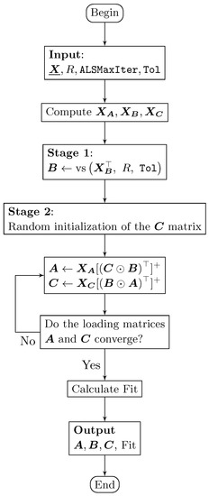 Figure 1. Flowchart of the DisjointParafacALS algorithm to compute a single disjoint orthogonal matrix ().
3.3. Algorithm and Flowchart
We summarize our proposal in Algorithm 2 to explain how the DisjointParafacALS algorithm works when performing a component analysis for three-way tables with the Parafac model. Computing the disjoint orthogonal components in Step 6 of Algorithm 2 simultaneously in two or three loading matrices is an approach that the analyst must choose. However, we do not recommend this approach due to the significant loss of fit that we have observed in the different computational experiments carried out. We suggest computing a single disjoint orthogonal loading matrix.
Note that the DisjointParafacALS algorithm can be utilized regardless of whether the degeneracy problem is present or not. This algorithm can be applied directly to a three-way table in order to interpret the loading matrices, with the corresponding loss of fit in the model; see Figure 2.
| Algorithm 2: Procedure for using the DisjointParafacALS algorithm |
|
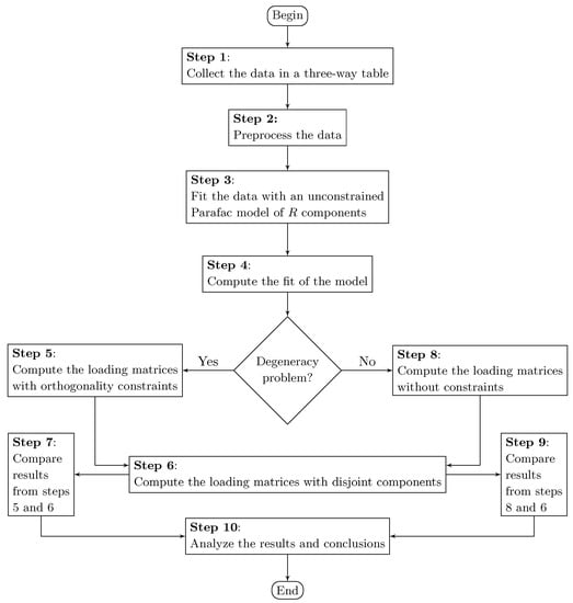
Figure 2.
Flowchart for using the DisjointParafacALS algorithm.
4. Computational Aspects
4.1. Characteristics of Hardware and Software
Table 3 shows the details of the software and hardware used in the implementation of the algorithms and in the computational experiments carried out.
Table 3.
Hardware and software used in computational experiments.
We must mention that the DisjointParafacALS algorithm requires more processing time (runtime) than the ParafacALS algorithm, even if the degeneracy problem is present. This is explained by the fact that calculating a disjoint orthogonal loading matrix consumes significant computational resources, which leads to longer processing time. The DisjointPCA, ParafacALS, and DisjointParafacALS algorithms that are presented in this paper were implemented mainly in C#.NET. For the particular case of the generation of random numbers, the SVD decomposition and the calculation of the generalized inverse of a matrix, the R statistical software was used.
4.2. Experimental Settings for Simulated Data
We designed and implemented a simulation algorithm to randomly build a three-way table with a disjoint latent structure of R components and its three modes, according to the Parafac model. Then, the DisjointParafacALS algorithm should be able to detect such a structure.
The loading matrices , and used in the numerical experiments related to the simulated data were generated as in [26]. In order to complete the creation of the random three-way table , the matrix equation was defined as
The matrix defined in (6) had the frontal slices of . The algorithm that buildt the three-way random table had to implement an application stated as
This was subject to: , , and . Note that is the set of all three-way tables with real entries. Additionally, it must satisfy that
where is the number of original individuals in the rth latent individual; is the number of original variables in the rth latent variable; and is the number of original locations in the rth latent location. The output defined in (7) is the three-way table that has a disjoint latent structure to be detected by the DisjointParafacALS algorithm.
4.3. Experimental Application with Simulated Data
We conducted computational experiments to evaluate the performance and benefits of the DisjointParafacALS algorithm. The first experiment corresponded to data simulated by an algorithm that was exclusively designed to generate three-way data with a disjoint structure according to the Parafac model. The other experiments are presented in the following section and related to (i) real data of evaluation of TV programs [30]; (ii) real data of perception of parents’ behavior by their children and by the parents themselves [31]; and (iii) real data from the study of tongue movements when speakers pronounce vowels in English [32].
Here, we show how the DisjointParafacALS algorithm works by using the application to generate the three-way random table . Specifically, consider the instance given by according to the definition of given in (7), with . Furthermore, constraints stated in (8) were satisfied. The other parameter setting was given by 10,000 and Tol . Table 4 shows the component correlation matrix from where we can conclude, based on the output, that the degeneracy problem was not present in the data.
Table 4.
Component correlation matrix for the simulated data.
The DisjointParafacALS algorithm was executed in three different situations. There are four execution scenarios. In the first scenario, the ParafacALS algorithm gave a fit of . In the second scenario, in which only the loading matrix was disjoint orthogonal, a fit of was obtained. In the third scenario, in which only the loading matrix was disjoint orthogonal, a fit of was obtained. In the last and fourth scenario, in which only the loading matrix was disjoint orthogonal, a fit of was obtained. These computational experiments are summarized in Table 5.
Table 5.
Disjoint orthogonal components, its fit (in %) and runtime (in minutes) for the indicated matrix with simulated data.
Table 6 reports the loading matrix for the second scenario. Observe that the DisjointParafacALS algorithm was able to detect the disjoint structure in the first mode.
Table 6.
Loading matrix with the DisjointParafacALS algorithm for the simulated data.
Table 7 presents the loading matrix for the third scenario. Note that indeed the DisjointParafacALS algorithm was able to assess the disjoint structure in the second mode.
Table 7.
Loading matrix with the DisjointParafacALS algorithm for the simulated data.
Table 8 shows the loading matrix for the fourth scenario. Notice that the DisjointParafacALS algorithm was able to identify the disjoint structure in the third mode.
Table 8.
Loading matrix with the DisjointParafacALS algorithm for the simulated data.
As observed in Table 6, Table 7 and Table 8, the disjoint structure facilitated the interpretation of the loading matrices, but with some loss of fit. In a fifth scenario, the DisjointParafacALS algorithm was executed with the loading matrices and set to be disjoint orthogonal as a constraint (illustration of a computational experiment with two disjoint orthogonal matrices). A fit of was obtained, that is, with two disjoint orthogonal matrices, we obtain a high loss of fit. In the rows of Table 6, Table 7 and Table 8 are the original entities, and in the columns are the latent entities.
We recommend running the DisjointParafacALS algorithm with a single disjoint orthogonal matrix as shown in Table 5, and where appropriate, running the DisjointParafacALS algorithm with two disjoint orthogonal matrices.
5. Applications with Real-World Data
5.1. Applying the DisjointParafacALS Algorithm to TV Data
We considered the well-known “TV data” set, where 30 university students classify 15 American programs using 16 bipolar scales. As noted in [15], the first mode corresponded to students, the second mode corresponded to bipolar scales and the third mode corresponded to TV programs. The full data set can be downloaded from the R package named ThreeWay.
A three component dimensional reduction with the Parafac model was chosen as in [30]. As part of the preprocessing, the three-way table was centered first with respect to scales (second mode) and then centered with respect to TV programs (third mode). Thus, normalization was applied with respect to the bipolar scales.
In the reported computational experiments, the following values were used: = 10,000 and Tol . When executing the ParafacALS algorithm with these data, the degeneracy problem was presented. After more than 7000 iterations, we obtained a fit of and the component correlation matrix stated in Table 9. In this table, the correlation between the components one and three was approximately , a result that suggests the presence of degeneracy. Furthermore, a high number of iterations (7231 iterations) was required to reach the stopping criterion of the ParafacALS algorithm. To solve the degeneracy problem, in [10], it is recommended to impose orthogonality constraints on at least one of the loading matrices. By imposing the orthogonality constraint on the loading matrix , a fit of was obtained in 239 iterations. The component correlation matrix obtained for is reported in Table 10.
Table 9.
Component correlation matrix for TV data.
Table 10.
Component correlation matrix with the orthogonal matrix for TV data.
Similarly to [15], in order to aid the interpretation, in this last execution, we set the columns of the loading matrices and to be unit vectors. Such a constraint was compensated in matrix . Then, the DisjointParafacALS algorithm was executed in two different scenarios. In the first of them, only the loading matrix had disjoint orthogonal components, but in the second scenario, only the loading matrix had disjoint orthogonal components. The fit obtained and the processing time in all executions is summarized in Table 11.
Table 11.
Comparison of fit and runtime for TV data.
Note that having disjoint orthogonal components affected the fit, but the interpretation increased, as we will illustrate later. As stated in [30], the three components could be interpreted as “humor”, “sensitivity” and “violence”. It should be noted that a negative value in loading matrix was interpreted as belonging to the left side of the bipolar scale. Table 12 shows the orthogonal loading matrix that was obtained using the ParafacALS algorithm. Table 13 reports the disjoint orthogonal matrix that was obtained with the DisjointParafacALS algorithm. Loadings with absolute values greater than or equal to that we observe in Table 12 and Table 13 facilitate comparison. Except for minor differences, the interpretation was the same.
Table 12.
Orthogonal loading matrix with the ParafacALS algorithm for TV data.
Table 13.
Disjoint orthogonal matrix with the DisjointParafacALS algorithm for TV data.
Table 14 presents the loading matrix that was obtained using the ParafacALS algorithm. Table 15 reports the disjoint orthogonal matrix that was reached with the DisjointParafacALS algorithm. Loadings with absolute values greater than or equal to reported in Table 14 and Table 15 facilitate comparison. Except for minor differences, the interpretation was the same.
Table 14.
Loading matrix with the ParafacALS algorithm for TV data.
Table 15.
Disjoint orthogonal matrix with the DisjointParafacALS algorithm for TV data.
5.2. Applying the DisjointParafacALS Algorithm to Kojima Data
A Parafac model was applied in [31]. The three-way table was a tensor with 153 Japanese girls in the first mode, 18 behavior scales in the second mode, and four judgements or conditions in the third mode. The full data set can be downloaded from http://three-mode.leidenuniv.nl (accessed on 9 July 2021).
With these data, we studied the perception of parents’ behavior by their children and by the parents themselves. To do so, the reactions of parents and children were received in parallel versions of the same questionnaire. The four conditions of the third mode were: FF (the father evaluates his own behavior), MM (the mother evaluates her own behavior), DF (the daughter evaluates the father’s behavior) and DM (the daughter evaluates the mother’s behavior).
The 18 scales were grouped into four types: Parental support or acceptance (PSA), behavioral and psychological control (BPC), rejection (R), and lax discipline (LD). As in [31], components were chosen. Furthermore, as part of the data preprocessing, a centering was performed in the first mode and then a normalization in the second mode. In the reported computational experiments, the following values were used: 10,000 and Tol . When executing the ParafacALS algorithm with these data, the degeneracy problem was once again presented. After more than iterations, we reached a fit of and the component correlation matrix is reported in in Table 16.
Table 16.
Component correlation matrix with components for Kojima data.
Table 16 tells us that the degeneracy problem could be present again. Components 1 and 3 had a high negative correlation (value close to ). In [31], the orthogonality condition of matrix was imposed. We proceed to assume that matrix must be disjoint orthogonal to improve the interpretation in the second mode and the DisjointParafacALS algorithm was used. We obtained that the component correlation matrix was the identity matrix. The DisjointParafacALS algorithm was executed in two different scenarios. In the first of these, only the loading matrix had disjoint orthogonal components with components, and in the second scenario, only the loading matrix had disjoint orthogonal components with components. Additionally, the ParafacALS algorithm was executed with components and the presence of the degeneration problem was also observed. Table 17 reports that components 2 and 3 had a high negative correlation. The DisjointParafacALS algorithm was used to solve the degeneracy problem with components. Then, we obtained that the component correlation matrix was the identity matrix. The fit obtained and the processing time in all executions are summarized in Table 18.
Table 17.
Component correlation matrix with components for Kojima data.
Table 18.
Comparison of fit and runtime for Kojima data.
We proceed to the analysis of the loading matrix for the scales. In Table 19, we see the three components calculated in [31]. Table 20 shows the three disjoint components calculated with the DisjointParafacALS algorithm. In Table 19, it is observed that the component 1 mainly groups the “parental support or acceptance” scales with high positive loadings and the “rejection” scales with high negative loadings. The component 2 mainly groups both, the “behavioral and psychological control” and “rejection” scales with high positive loadings, the second one with lower values. In the component 3, we observe some “behavioral and psychological control” scales with high positive loadings. The “lax discipline” scales are not related with any particular component.
Table 19.
Matrix obtained by the orthogonal matrix condition for Kojima data.
Table 20.
Disjoint orthogonal matrix using components and obtained with the DisjointParafacALS algorithm for Kojima data.
When analyzing the three components, note that component 1 represents the “parental support or acceptance” scales. The component 2 groups “behavioral and psychological control” and “rejection”. The component 3 is represents “lax discipline”. Table 21 reports what happens if four disjoint components are computed with the DisjointParafacALS algorithm. The components 1, 2, 3 and 4 group “parental support or acceptance”, “behavioral and psychological control”, “rejection" and “lax discipline” scales, respectively.
Table 21.
Disjoint orthogonal matrix using components and obtained with the DisjointParafacALS algorithm for Kojima data.
5.3. Applying the DisjointParafacALS Algorithm to Tongue Data
In [32], a study was carried out with the Parafac model about the position of certain points of the tongue while some speakers pronounced different vowels in English. These data were stored in the three-way table . The first mode corresponded to 10 vowels in English, the second mode corresponded to 13 predefined points of the tongue and the third mode corresponded to five speakers. To generate the data, x-rays were taken on five people while they pronounced the 10 vowels. The full data set is in [32].
Two components were chosen () and a centering was carried out in the first mode. In the reported computational experiments, the following values were used: 10,000 and Tol . Table 22 presents the fit obtained and the execution time in four scenarios. In the first one, no disjoint orthogonal components were computed. From the component correlation matrix observed in Table 23, the presence of the degeneracy problem is not suspected now. In the other three scenarios, disjoint orthogonal components were calculated for the loading matrices , and , respectively. In addition, in the last three scenarios, the component correlation matrix is the identity matrix.
Table 22.
Comparison of fit and runtime for tongue data.
Table 23.
Component correlation matrix with components for tongue data.
From Table 24, observe that vowels 1, 2, 3 and 4 are better represented in the first component with positive loadings. Furthermore, vowels 8 and 9 were also better represented in the first component but with negative loadings. In addition, vowels 5 and 6 were better represented in the second component with negative loadings and vowel 10 was better represented in the second component with positive loading. When interpreting the disjoint components of Table 25, we conclude the same as in [32]. Vowel 7 had loadings less than in both components in Table 24, but the DisjointParafacALS algorithm placed vowel 7 in the first component with negative loading.
Table 24.
Loading matrix with the ParafacALS algorithm for tongue data.
Table 25.
Disjoint orthogonal matrix with the DisjointParafacALS algorithm for tongue data.
Table 26 shows the components calculated in [32]. The first component was mainly related to large movements of the points of the tongue located in the front of the mouth, while the second component was mainly associated with larger movements of the points of the tongue located in the back of the mouth. In the analysis with disjoint components (see Table 27), note that the tongue points 11 to 16, which were the closest to the mouth, were represented in the first component with positive loadings. Tongue points 4 to 7, which were the points that are further from the mouth, were in the first component with negative loadings. Furthermore, the tongue points 8, 9 and 10 located in the back of the mouth were represented in the second component with negative loadings.
Table 26.
Loading matrix with the ParafacALS algorithm for tongue data.
Table 27.
Disjoint orthogonal matrix with the DisjointParafacALS algorithm for tongue data.
As a reference, keep in mind that the tongue point 4 was located near the epiglottis (in the throat behind the tongue) and the other tongue points were located upwards in the direction of the mouth ending at point 16 which was located near the lips.
In Table 28, the speakers 1, 2 and 5 have negative loadings and are better represented in the first component. Furthermore, speaker 4 also has negative loading and is better represented in the second component, just as we see in Table 29 where we have the disjoint components. Speaker 3 has similar values in the two components of Table 28, but the DisjointParafacALS algorithm places speaker 3 in the second component with negative loading.
Table 28.
Loading matrix with the ParafacALS algorithm for tongue data.
Table 29.
Disjoint orthogonal matrix with the DisjointParafacALS algorithm for tongue data.
6. Conclusions, Other Potential Applications, and Future Work
One of the most popular models for component analysis in three-way tables is the Parafac model. However, a big problem with the existing techniques in the Parafac model is that interpretable loading matrices are not always obtained.
In the present study, a novel heuristic algorithm for computing disjoint orthogonal components in a three-way table with the Parafac model was proposed. This algorithm mixes the ParafacALS and disjoint PCA algorithms. The computational experiments reported that the main benefit of the algorithm is the easier interpretation of the loading matrices. In addition, the algorithm permited us to analyze a three-way table when the degeneracy problem exists. Such experiments indicated that the algorithm identifies and catches disjoint structures in a three-way table with the Parafac model. These experiments based on simulated and real data sets enabled us to demonstrate the good performance and potential applications of the new algorithm. This algorithm may be a helpful multivariate tool for practitioners, applied statisticians, and data scientists.
A limitation of our algorithm is that it does not guarantee an optimal solution. When additional constraints to those present in the original problem are absent, the feasible solutions state the global optimum. However, if the constraints of the DisjointParafacALS algorithm are incorporated, the feasible solutions are compressed, reaching a solution close to the global optimum. Therefore, the fit for the solution given by the algorithm is less than the fit of the ParafacALS algorithm. Nevertheless, the built-in constraints permit us to add zeros in the positions of the variables with low contribution in a component of the loading matrix, allowing the interpretation of the components more clearly. The new algorithm takes longer than the ParafacALS algorithm, even when the degeneracy problem is present in the data, so there is a trade-off between interpretation and speed.
In order to motivate practitioners, the new algorithm can be applied to:
- (i)
- Marketing and sales, for example in the selection of an appropriate commercial spoken for a given brand [8,21].
- (ii)
- The Parafac model also has applications in chemistry (chromatography, fluorescence spectroscopy, food industry, and second-order calibration) [33,34,35].
- (iii)
- There are also applications in environmental sciences related to water [36].
- (iv)
- The Parafac model is also used in psychometry [11,31].
Some open problems that arose from this study and that authors are analyzing are the following. We think that the disjoint method may be employed together with other existing methods to improve its performance, as in the multidimensional scaling of three-way data. Also, bootstrapping for the loading matrices of the Parafac model may be used. In addition, there exists a wide field of usages in statistical learning. Computing disjoint orthogonal components in higher order tensors is also a challenge.
Author Contributions
Data curation, X.C., J.A.R.-F., C.M.-B.; investigation, C.M.-B., M.P.G.-V.; formal analysis and methodology, C.M.-B., J.A.R.-F., X.C., V.L., A.M.-C., M.P.G.-V.; writing—original draft, C.M.-B., J.A.R.-F., X.C., V.L., A.M.-C., M.P.G.-V.; writing—review and editing, V.L., C.M.-B., X.C. All authors have read and agreed to the published version of the manuscript.
Funding
This research was partially supported by FONDECYT, project grant number 1200525 (V.L.), from the National Agency for Research and Development (ANID) of the Chilean government under the Ministry of Science, Technology, Knowledge, and Innovation.
Institutional Review Board Statement
Not applicable.
Informed Consent Statement
Not applicable.
Data Availability Statement
The data analyzed are available from the authors upon request.
Acknowledgments
The authors would also like to thank the editor and reviewers for their constructive comments which led to improving the presentation of the manuscript.
Conflicts of Interest
The authors declare no conflict of interest.
References
- Hached, M.; Jbilou, K.; Koukouvinos, C.; Mitrouli, M. A multidimensional principal component analysis via the C-product Golub–Kahan–SVD for classification and face recognition. Mathematics 2021, 9, 1249. [Google Scholar] [CrossRef]
- Martin-Barreiro, C.; Ramirez-Figueroa, J.A.; Cabezas, X.; Leiva, V.; Galindo-Villardón, M.P. Disjoint and functional principal component analysis for infected cases and deaths due to COVID-19 in South American countries with sensor-related data. Sensors 2021, 21, 4094. [Google Scholar] [CrossRef]
- Hitchcock, F.L. The expression of a tensor or a polyadic as a sum of products. J. Math. Phys. 1927, 6, 164–189. [Google Scholar] [CrossRef]
- Hitchcock, F.L. Multiple invariants and generalized rank of a p-way matrix or tensor. J. Math. Phys. 1927, 7, 39–79. [Google Scholar] [CrossRef]
- Harshman, R.A. Foundations of the Parafac procedure: Models and conditions for an explanatory multimodal factor analysis. UCLA Work. Pap. Phon. 1970, 16, 1–84. [Google Scholar]
- Carroll, J.D.; Chang, J.J. Analysis of individual differences in multidimensional scaling via an N-way generalization of “Eckart-Young” decomposition. Psychometrika 1970, 35, 283–319. [Google Scholar] [CrossRef]
- Bro, R.; Kiers, H.A.L. A new efficient method for determining the number of components in Parafac models. J. Chemom. 2003, 17, 274–286. [Google Scholar] [CrossRef]
- Harshman, R.A.; Desarbo, W.S. An Application of Parafac to a Small Sample Problem, Demonstrating Preprocessing, Orthogonality Constraints, and Split-Half Diagnostic Techniques. In Research Methods for Multimode Data Analysis; Law, H.G., Snyder, C.W., Jr., Hattie, J.A., McDonald, R.P., Eds.; Praeger: New York, NY, USA, 1984; pp. 602–642. [Google Scholar]
- Leardi, R. Multi-Way Analysis with Applications in the Chemical Sciences, Age Smilde; Bro, R., Geladi, P., Eds.; Wiley: Chichester, UK, 2004. [Google Scholar]
- Harshman, R.; Lundy, M.E. Data preprocessing and the extended Parafac model. In Research Methods for Multimode Data Analysis; Law, H.G., Snyder, C.W., Jr., Hattie, J.A., McDonald, R.P., Eds.; Praeger: New York, NY, USA, 1984; pp. 216–284. [Google Scholar]
- Kroonenberg, P. Applied Multiway Data Analysis; Wiley: New York, NY, USA, 2008. [Google Scholar]
- Smilde, A.; Geladi, P.; Bro, R. Multi-Way Analysis: Applications in the Chemical Sciences; Wiley: New York, NY, USA, 2005. [Google Scholar]
- Amigo, J.M.; Marini, F. Multiway methods. In Data Handling in Science and Technology; Elsevier: Amsterdam, The Netherlands, 2011; Volume 28, pp. 265–313. [Google Scholar]
- Favier, G.; de Almeida, A.L. Overview of constrained Parafac models. EURASIP J. Adv. Signal Process. 2014, 2014, 142. [Google Scholar] [CrossRef]
- Giordani, P.; Kiers, H.; Ferraro, M.D. Three-way component analysis using the R package threeWay. J. Stat. Softw. Artic. 2014, 57, 1–23. [Google Scholar]
- Papalexakis, E.; Faloutsos, C.; Sidiropoulos, N.D. ParCube: Sparse parallelizable tensor decompositions. In Machine Learning and Knowledge Discovery in Databases; Springer: Berlin, Germany, 2012; pp. 521–536. [Google Scholar]
- Kaya, O.; Ucar, B. Scalable sparse tensor decompositions in distributed memory systems. In Proceedings of the International Conference for High Performance Computing, Networking, Storage and Analysis, Austin, TX, USA, 15–20 November 2015; pp. 1–11. [Google Scholar]
- Li, J.; Ma, Y.; Wu, X.; Li, A.; Barker, K. PASTA: A parallel sparse tensor algorithm benchmark suite. CCF Trans. High Perform. Comput. 2019, 1, 111–130. [Google Scholar] [CrossRef]
- Kiers, H.A.; Giordani, P. Candecomp/Parafac with zero constraints at arbitrary positions in a loading matrix. Chemom. Intell. Lab. Syst. 2020, 207, 104145. [Google Scholar] [CrossRef]
- Wilderjans, T.F.; Ceulemans, E. Clusterwise Parafac to identify heterogeneity in three-way data. Chemom. Intell. Lab. Syst. 2013, 129, 87–97. [Google Scholar] [CrossRef]
- Cariou, V.; Wilderjans, T.F. Consumer segmentation in multi-attribute product evaluation by means of non-negatively constrained CLV3W. Food Qual. Prefer. 2018, 67, 18–26. [Google Scholar] [CrossRef]
- Vichi, M.; Saporta, G. Clustering and disjoint principal component analysis. Comput. Stat. Data Anal. 2009, 53, 3194–3208. [Google Scholar] [CrossRef]
- Macedo, E.; Freitas, A. The alternating least-squares algorithm for CDPCA. In EURO Mini-Conference on Optimization in the Natural Sciences; Plakhov, A., Tchemisova, T., Freitas, A., Eds.; Springer: Cham, Switzerland, 2015; pp. 173–191. [Google Scholar]
- Ferrara, C.; Martella, F.; Vichi, M. Dimensions of well-being and their statistical measurements. In Topics in Theoretical and Applied Statistics; Springer: Cham, Switzerland, 2016; pp. 85–99. [Google Scholar]
- Ramirez-Figueroa, J.A.; Martin-Barreiro, C.; Nieto-Librero, A.B.; Leiva, V.; Galindo-Villardón, M.P. A new principal component analysis by particle swarm optimization with an environmental application for data science. Stoch. Environ. Res. Risk Assess. 2021. [Google Scholar] [CrossRef]
- Martin-Barreiro, C.; Ramirez-Figueroa, J.A.; Nieto-Librero, A.B.; Leiva, V.; Martin-Casado, A.; Galindo-Villardón, M.P. A new algorithm for computing disjoint orthogonal components in the three-Way Tucker model. Mathematics 2021, 9, 203. [Google Scholar] [CrossRef]
- Kolda, T.G.; Bader, B.W. Tensor decompositions and applications. SIAM Rev. 2009, 51, 455–500. [Google Scholar] [CrossRef]
- Tomasi, G.; Bro, R. A comparison of algorithms for fitting the Parafac model. Comput. Stat. Data Anal. 2006, 50, 1700–1734. [Google Scholar] [CrossRef]
- Caro-Lopera, F.J.; Leiva, V.; Balakrishnan, N. Connection between the Hadamard and matrix products with an application to matrix-variate Birnbaum–Saunders distributions. J. Multivar. Anal. 2012, 104, 126–139. [Google Scholar] [CrossRef]
- Lundy, M.E.; Harshman, R.; Kruskal, J. A two stage procedure incorporating good features of both trilinear and quadrilinear models. In Multiway Data Analysis; Elsevier: Amsterdam, The Netherlands, 1989; pp. 123–130. [Google Scholar]
- Kroonenberg, P.M.; Harshman, R.A.; Murakami, T. Analysing three-way profile data using the Parafac and Tucker3 models illustrated with views on parenting. Appl. Multivar. Res. 2009, 13, 5–41. [Google Scholar] [CrossRef][Green Version]
- Harshman, R.; Ladefoged, P.; Goldstein, L. Factor analysis of tongue shapes. J. Acoust. Soc. Am. 1977, 62, 693–707. [Google Scholar] [CrossRef] [PubMed]
- Andersen, C.M.; Bro, R. Practical aspects of Parafac modeling of fluorescence excitation-emission data. J. Chemom. 2003, 17, 200–215. [Google Scholar] [CrossRef]
- Bro, R.; Heimdal, H. Enzymatic browning of vegetables. Calibration and analysis of variance by multiway methods. Chemom. Intell. Lab. Syst. 1996, 34, 85–102. [Google Scholar] [CrossRef]
- Bro, R. Exploratory study of sugar production using fluorescence spectroscopy and multi-way analysis. Chemom. Intell. Lab. Syst. 1999, 46, 133–147. [Google Scholar] [CrossRef]
- Leardi, R.; Armanino, C.; Lanteri, S.; Alberotanza, L. Three-mode principal component analysis of monitoring data from Venice lagoon. J. Chemom. 2000, 14, 187–195. [Google Scholar] [CrossRef]
Publisher’s Note: MDPI stays neutral with regard to jurisdictional claims in published maps and institutional affiliations. |
© 2021 by the authors. Licensee MDPI, Basel, Switzerland. This article is an open access article distributed under the terms and conditions of the Creative Commons Attribution (CC BY) license (https://creativecommons.org/licenses/by/4.0/).