Using an Improved Differential Evolution for Scheduling Optimization of Dual-Gantry Multi-Head Surface-Mount Placement Machine

Abstract

The difference between dual-gantry and single-gantry surface-mount placement (SMP) machines is that dual-gantry machines exhibit higher complexity and more problems due to their additional gantry robot, such as component allocation and collision. This paper presents algorithms to prescribe the assembly operations of a dual-gantry multi-head surface-mount placement machine. It considers five inter-related problems: (i) component allocation; (ii) automatic nozzle changer assignment; (iii) feeder arrangement; and (iv) pick-and-place sequence; it incorporates a practical restriction related to (v) component height. The paper proposes a solution to each problem: (i) equalizing “workloads” assigned to the gantries, (ii) using quantity ratio method, (iii) using two similarity measurement mechanisms in a modified differential evolution algorithm with a random-key encoding mapping method that addresses component height restriction, (iv) and a combination of nearest-neighbor search and 2-opt method to plan each placing operation. This study reports an experiment that involved the processing of 10 printed circuit boards and compared the performance of a modified differential evolution algorithm with well-known algorithms including differential evolution, particle swarm optimization, and genetic algorithm. The results reveal that the number of picks, moving distance of picking components, and total assembly time with the modified differential evolution algorithm are less than other algorithms.

1. Introduction

Recently, the number of components placed on high-density printed circuit boards (PCBs) has been increasing, which has resulted in the increased use of surface-mount technology (SMT) during the production process of PCBs. Machines with SMT are called surface-mount placement (SMP) machines, which are advantageous for their precision, speed, and efficiency in PCB production compared with manual assembly methods. Therefore, manual assembly methods have been gradually replaced by SMP machines.

To simplify the complexity of such assembly problems, most studies on scheduling optimization for dual-gantry SMP machines have overlooked various limitations, such as problems related to automatic nozzle changer (ANC) assignment, nozzle setup, and height restrictions for components. Optimization of dual-gantry multi-head SMP machines creates various problems, and the main problem affecting operating efficiency is divided into three sub-problems, namely the component allocation problem, the feeder arrangement problem, and the component pick-and-place sequence problem. These problems are nondeterministic-polynomial (NP)-hard problems, which are high-dimensional and discrete; thus, an optimal global solution is difficult to obtain using conventional methods.

Production scheduling is a decision-making process that plays a critical role in manufacturing and production systems and has a markedly positive impact on the performances of manufacturing. Effective scheduling can result in improvements in throughput, inventory costs, utilization of manufacturing resources, and energy saving. In the past decades, various scheduling problems have been extensively solved by multi-population meta-heuristics such as artificial bee colony (ABC), imperialist competitive algorithm (ICA), and shuffled frog-leaping algorithm (SFLA). SMP scheduling is no exception; to optimize the dual-gantry multi-head SMP machine, scholars have proposed numerous approaches to solve the component allocation problem, the feeder arrangement problem, and the component pick-and-place sequence problem. Sun et al. [1] employed a genetic algorithm to optimize component allocation and feeder arrangement problems by maximizing the number of simultaneously picked-up components or equivalently minimizing the number of pickups, and equalizing workloads assigned to heads. Du and Li [2] combined heuristic method with genetic algorithm to optimize the placement process by minimizing the displacement of gantry and equalizing the workload between two gantries. Additionally, Ashayeri, Ma and Sotirov [3] developed a hierarchical approach of two stages for the multi-head surface-mounting device placement optimization problem. The first stage employed a mixed integer program model to decide the optimal sequence of batches of components to the placement heads. Then, the second stage was to determine the sequence of components using a heuristic method. The experimental results revealed that a near optimal solution was reached in reasonable computation time based on this hierarchical approach. Torabi et al. [4] formulated an integrated mathematical model to balance workloads over multiple heads. Firstly, the original bi-objective model was solved for small problem instances by the augmented ε-constraint method. Next, a multi-objective particle swarm optimization, tuned by Taguchi method, was introduced to generate a set of efficient solutions for medium- and large-sized problem instances. Zhu and Zhang [5] improved the basic shuffled frog-leaping algorithm (SFLA) for component pick-and-place sequence of the gantry multi-head surface-mounting machine. The three-way ANOVA was evaluated in parameters analyzing the improved SFLA; however, the experimental results noted that the advantages of improving SFLA were realized at the cost of CPU time. He et al. [6] innovated a hierarchical restricted balance (HRB) heuristic method to determine the optimal nozzle and feeder decisions in order to minimize the moving distance of gantries of a dual-delivery SMT placement machine. In optimization processing, the nozzle and feeder setups were searched using simulated annealing, and the pick-and-place sequence was solved by nearest neighbor and cheapest insertion heuristics. The results indicated that the HRB strategy improves the solution quality without increasing the computational time. Li and Yoon [7] proposed an adaptive nearest-neighbor tabu search to minimize the gantry moving distance in a high-speed single-gantry surface-mount device machine. The relationship among nozzle assignment, nozzle exchange scheduling, and the number of pick-and-place cycles was also analyzed in this study. The experimental results also declared that the proposed algorithm produced a 23.32% distance saving on average for the single-nozzle-type problem in comparison with the large clusters of operations heuristic method. He et al. [8] introduced workload balance between gantries and gantry cycle scheduling two decisions, and then the proposed heuristic multi-phase approach was used to minimize the moving distance of gantries by balancing the workload of a dual-delivery SMT placement machine. Huang et al. [9] developed a hierarchical multi-objective optimization model which set the nozzle optimization as an integer programming optimization model for the first master hierarchy. Additionally, component mounting sequence, feeder optimization and picking order are parallel-optimized based on the first hierarchy optimization as second hierarchical. Lastly, the authors proposed related algorithm strategies for the respective problems.

Table 1. Summary of the discussed problem in the related studies.

	Component Allocation	ANC Assignment	Feeder Arrangement	Component Height	Pick-and-Place Sequence	Method
Sun et al. [1]	✓		✓		✓	GA
Du and Li [2]	✓		✓		✓	Hybrid GA
Ashayeri et al. [3]	✓	✓			✓	MIP
Torabi et al. [4]	✓		✓		✓	MOPSO
Zhu and Zhang [5]					✓	ISFLA
He et al. [6]	✓	✓	✓		✓	HRB
Li and Yoon [7]		✓	✓		✓	ANNTS
He et al. [8]	✓		✓		✓	HS
Huang et al. [9]	✓		✓		✓	HMO
This study	✓	✓	✓	✓	✓	MDE

GA: genetic algorithm, MIP: mixed-integer program, MOPSO: multi-objective particle swarm optimization, ISFLA: improved basic shuffled frog-leaping algorithm, HRB: hierarchical restricted balance, ANNTS: adaptive nearest-neighbor tabu search, HS: hierarchical strategy, and HMO: hierarchical multi-objective.

displays the discussed problems of related studies.

As shown in Table 1, most of the previous studies [1,2,4,8,9] have already considered problems such as component allocation, feeder arrangement, and pick-and-place sequence during surface-mount placement processing. Among those, many different evolutionary algorithms were applied to optimize SMP processing. Afterward, ANC assignment problem was also included as a part of optimization factors [3,6,7]. In those studies, algorithms were established in a hybrid way to improve the shortcomings of single algorithms. Nevertheless, the height of the component can also have a direct effect on the manufacturing process. When placing the components on a PCB, the relatively lower components have to be placed first; therefore, unlike those methods, the current study included the consideration of the height restrictions in SMP processing and proposed an effective modified differential evolution (MDE) algorithm to optimize the scheduling of SMP machines in order to cover processing problems more comprehensively.

Research objectives of this present study incorporate problems of (i) component allocation, (ii) ANC assignment, (iii) feeder arrangements, (iv) pick-and-place sequences, and (v) height restrictions for components into the proposed solutions on minimizing the total assembly time for PCB assembly. The major contributions of this study are listed as follows:

♦

The component height restriction is considered in SMP processing.

♦

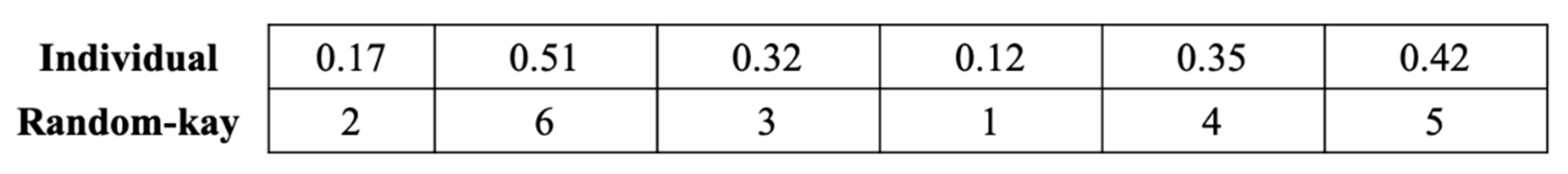
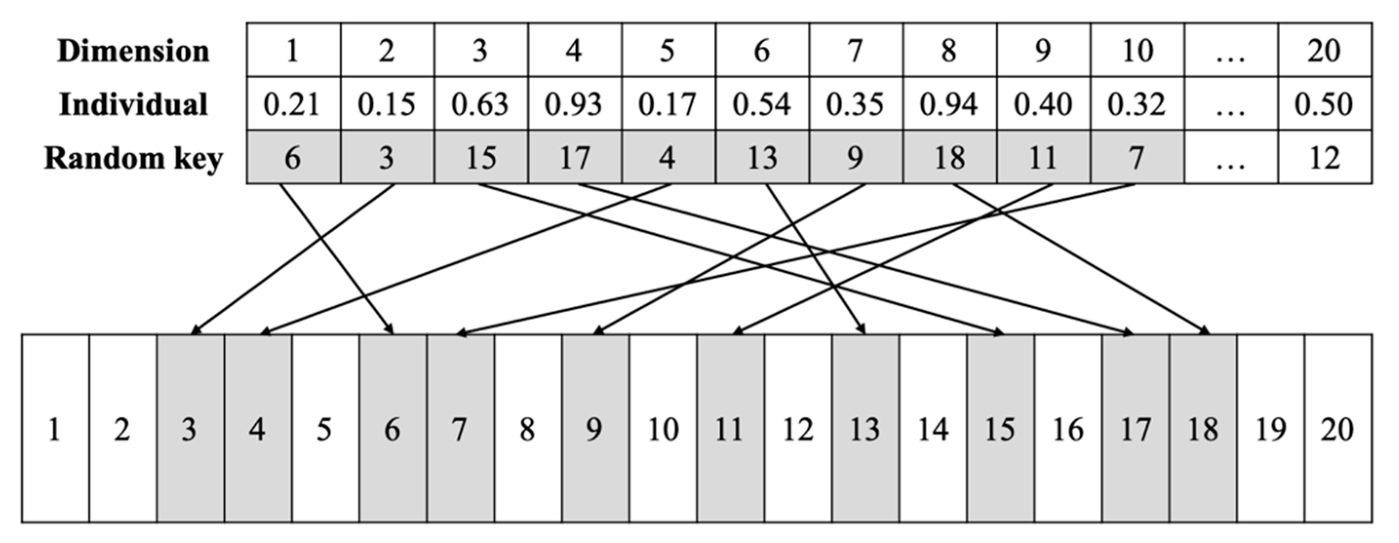
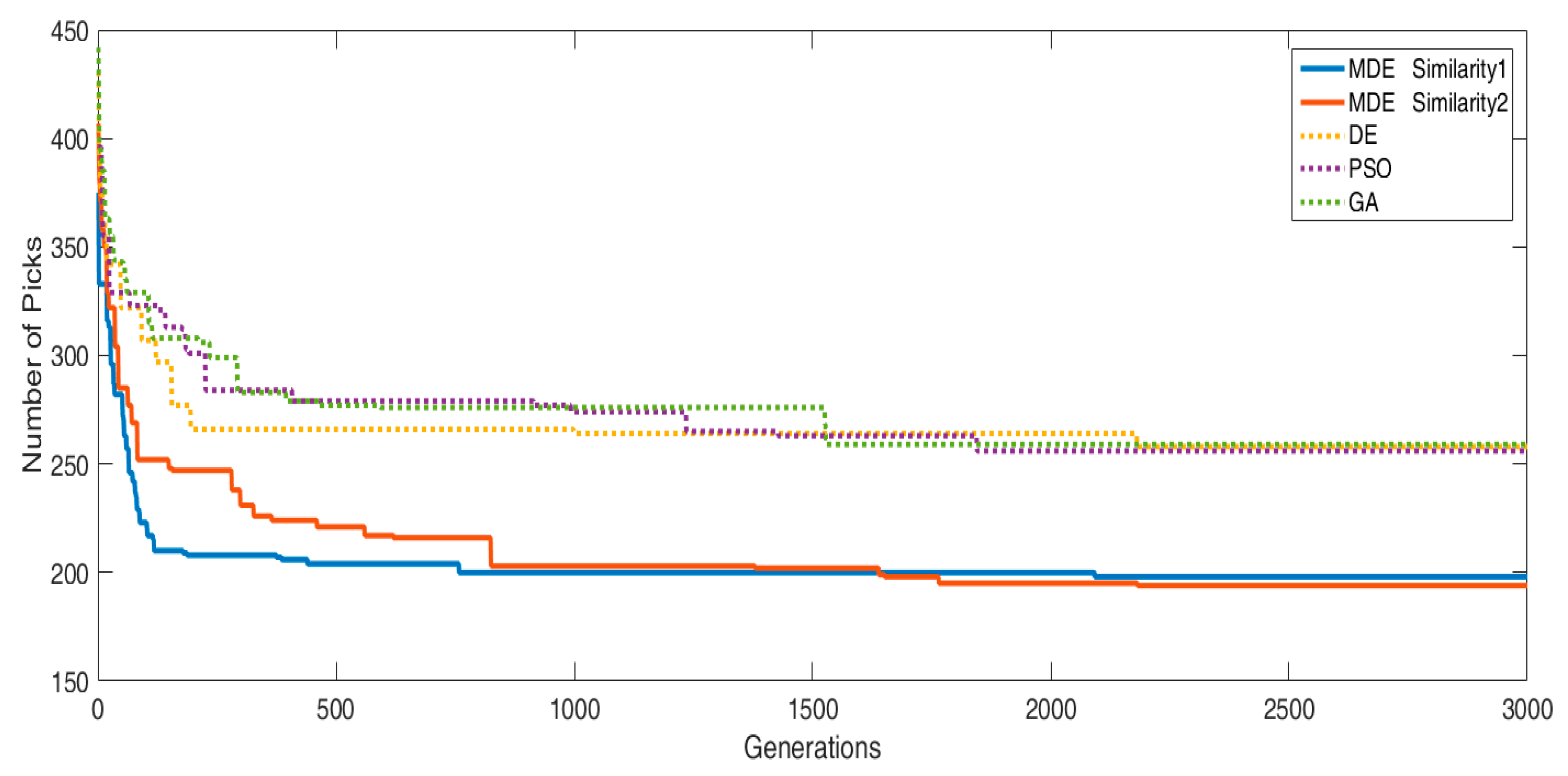
The proposed modified differential evolution (MDE) algorithm with two similarity measurement mechanisms using a random-key encoding mapping method is designed for minimizing the number of picks in feeder arrangement.

♦

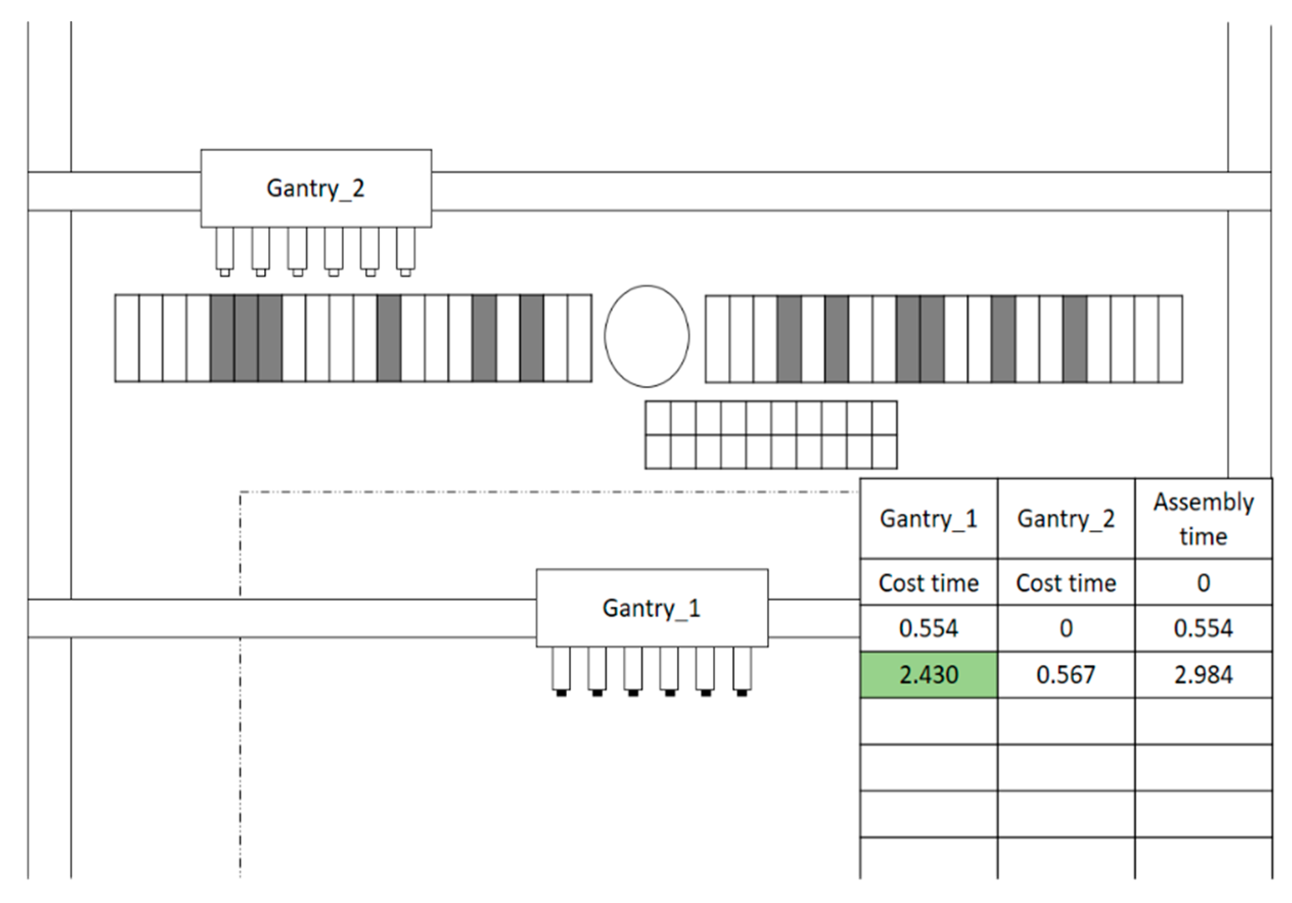
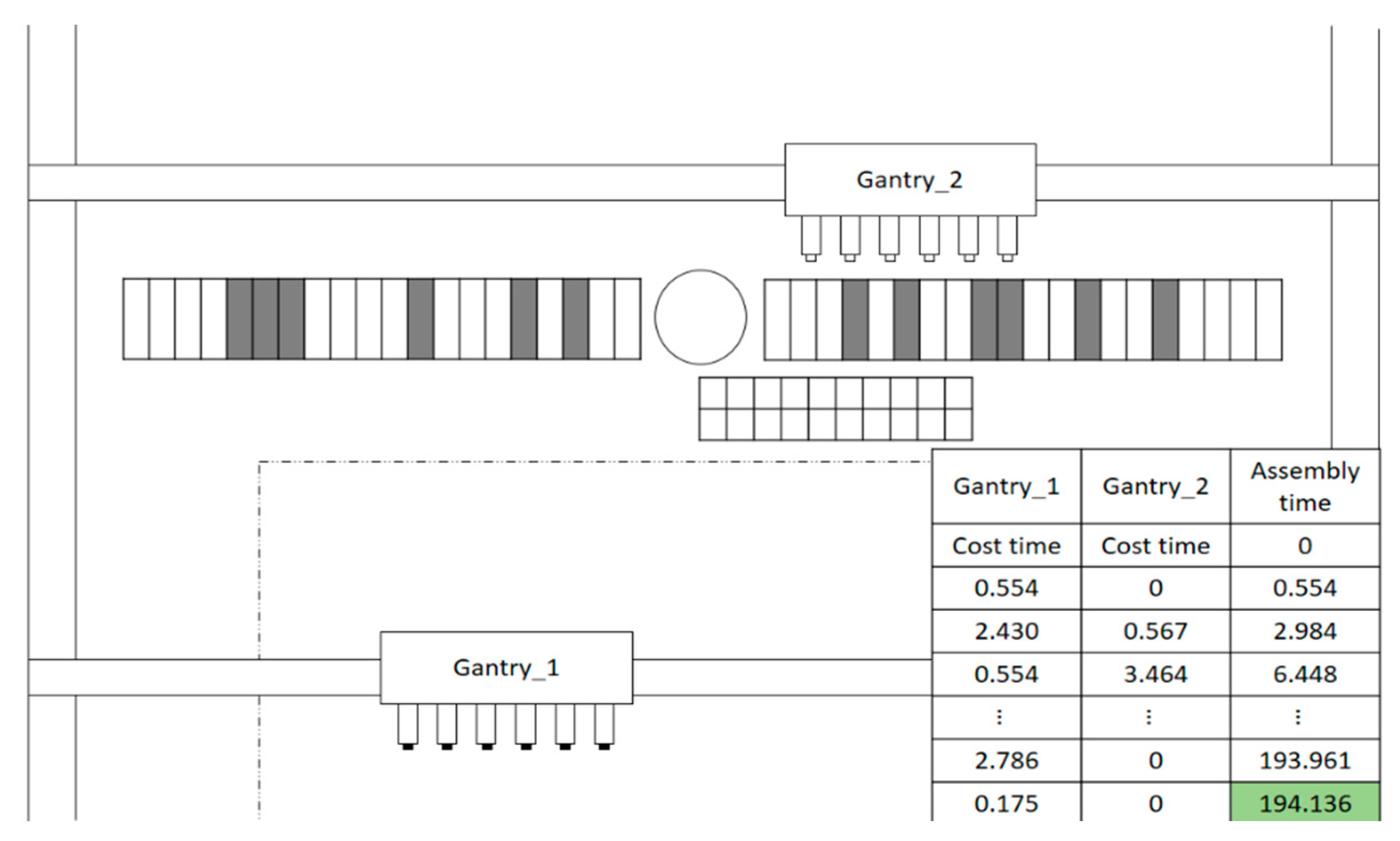
A combination of nearest-neighbor search (NNS) and 2-opt method is applied to shorten the path in component placing operations.

♦

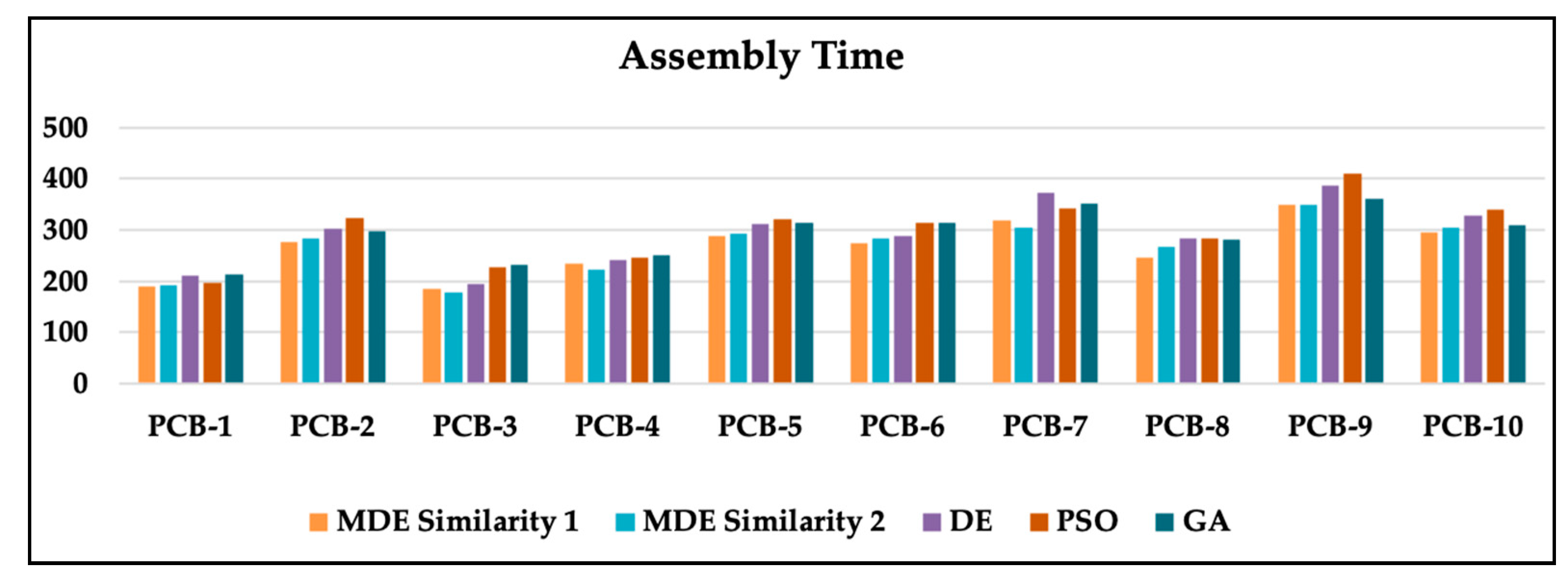
The experimental results indicate that while using the MDE algorithm for feeder arrangement, at most 30% of the number of picks can be reduced; moreover, when adding a combination of NNS and 2-opt method for component placing sequence, the whole assembly time is decreased at most by 13% using the proposed method.

The remainder of this article is structured as follows: Section 2 describes key features of the SMP machine. Section 3 presents the problem definitions. Section 4 introduces the methodology of whole processing including component allocation, ANC assignment, feeder arrangement using the proposed MDE algorithm, component picking sequence, and component placing sequence using NNS and 2-opt method. Section 5 details the experimental results and discussions. Finally, Section 6 gives the conclusions.

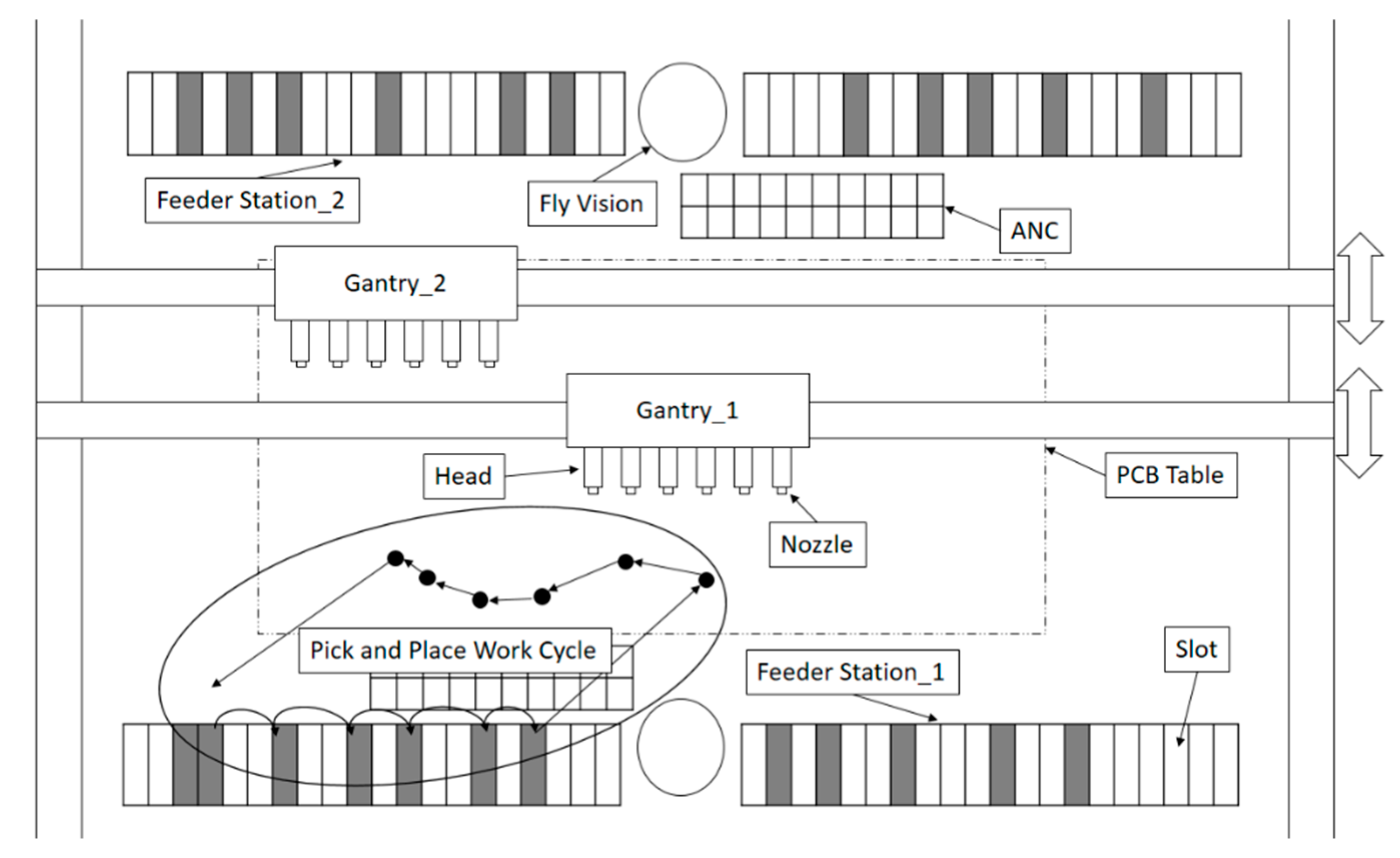
2. Description of the SMP Machine

A dual-gantry multi-head SMP machine (Figure 1) employs two robot gantries, each of which contains six pick-and-place heads. Each head is equipped with one nozzle and moves to the ANC for nozzle changes when required. During operation, robot gantries move to the feeder stations to pick components. As illustrated in Figure 1, Gantry_1 picks components from the feeder station_1, and Gantry_2 picks components from the feeder station_2. The two gantries then carry the picked components and place them on a PCB alternately. This operating process is known as a pick-and-place work cycle.

The SMP machine’s key features are as follows:

(a)

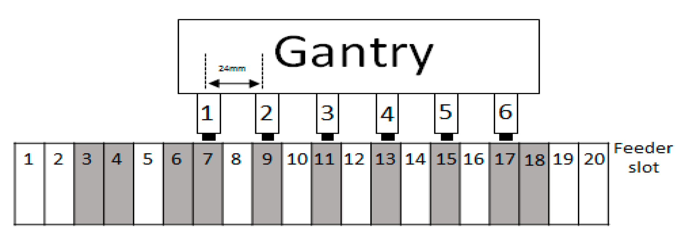
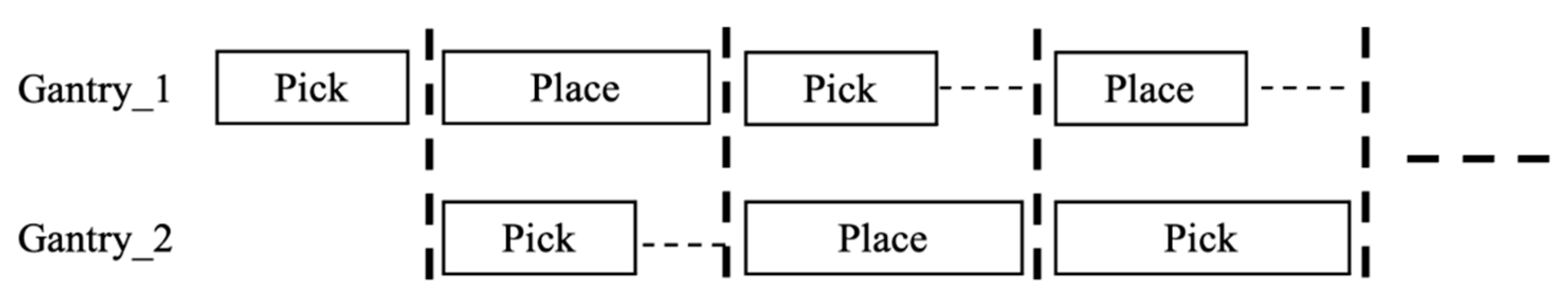
Gantry: This moves above the surface-mount machine, allowing the pick-and-place heads to pick components from the correct feeder and then to place the components on the correct position of the PCB.

(b)

Pick-and-place head: Every pick-and-place head is equipped with a single nozzle, which is used to pick and place components.

(c)

ANC: This is where nozzles are placed and changed.

(d)

Nozzle: These are installed on pick-and-place heads for component picking and placing. Different nozzle types are required for different components. Accordingly, the pick-and-place heads move to the ANC for nozzle changes when required.

(e)

Feeder: The feeder is used to store and provide components. Every feeder stores only one component.

(f)

Feeder station: Feeders for placement operation here.

(g)

PCB table: PCBs are fixed and placed here.

(h)

Fly vision system: This is used to determine whether a component is damaged or faulty and confirm a component’s loading position by recalibrating the X–Y coordinate.

Figure 2 presents the picking sequence {7, 9, 11, 13, 15, 17} that finished picks when the least number of picks is one. If the component picking operations cannot be finished in one pick, the picking operation is repeated until all heads pick their components or until it is determined that the operation cannot proceed any further. As presented in Figure 3, a head is idle after the first pick. Thus, the second pick is conducted, with its picking sequence being {3, 3, 7, 9, 9, 13}.

3. Problem Definition

3.1. Problem Description

The purpose of this study was to optimize the operation of dual-gantry, multi-head SMP machines. The following section introduces problems, inter-relationships of problems, and their influences on SMP operations.

(i)

Component allocation problem:

Each gantry has its own feeder station. Gantry_1 cannot pick components from Gantry_2’s feeder station and vice versa. An inappropriate component allocation may lead to an excessive workload on one of the gantries, thus causing workload imbalance.

(ii)

ANC assignment problem:

The dual-gantry, multi-head SMP machine that we studied with an ANC comprising 20 seats was designed for 16 small nozzles and 4 large nozzles. Because the number of nozzles placed in an ANC is limited, how to allocate the number of seats for each nozzle type is crucial. It affects component picking process. A greater number of picks indicates a longer time required for the picking process.

(iii)

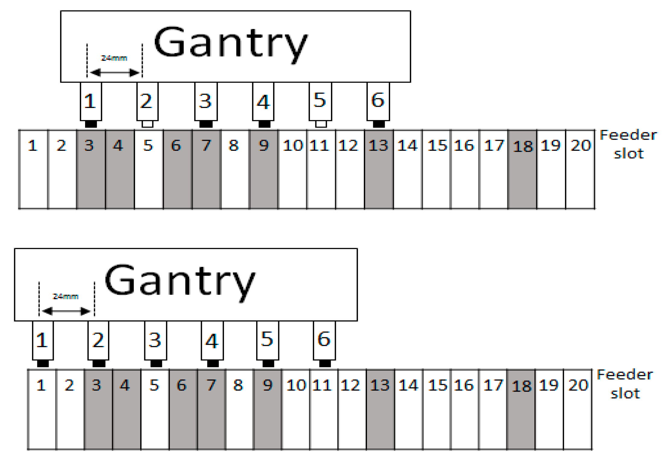
Feeder arrangement problem:

The assignment of components to the two feeder-slot stations for component storage mainly affects the picking process. Fewer picks indicate a shorter time required for this process. Therefore, an appropriate feeder arrangement enables picking up more components simultaneously, thus shortening the time required for this process.

(iv)

Component height restrictions:

Because the height of each component varies, placing an excessively high component before placing a shorter component leads to a collision. Therefore, the picking-and-placing order of components should be sequenced according to height (from low to high), in which the height differences between each two consecutive components should be less than 2 mm to avoid collision.

(v)

Component pick-and-place sequence:

Planning the shortest route for gantries to move from feeder-slot stations, where they pick components, to the position on PCBs to place components.

3.2. Establishment of a Mathematical Model

This study designed a mathematical model to calculate scheduling results according to the operation pattern of a dual-gantry multi-head SMP machine. We divided the entire operating process into four parts for discussion: number of cycles, pick time, placement time, and ANC change time.

Definition of symbols:

a: time required for a nozzle change

A: location of the ANC carrying replacement nozzle

c: cycle number, c = 1, 2, …, N

cn: number of nozzles needs to be changed, depends on sequence of picks

$d\left(S_p^c,S_{p+1}^c\right)$: moving distance of a head from location $S_p^c$ to $S_{p+1}^c$

E: time required for picking component

F: time required for placing component

g: the gantry being used. g = 1 for Gantry_1; g = 2 for Gantry_2

i: the numerical order in which components are arranged in a particular cycle, i = 1, 2, …

j: the last component placed in a cycle

o: waiting time for placing component

p: index for picks

P: loading location on a semi-finished PCB

S: location of the slot to which the components to be picked have been assigned in the feeder station

$T_{chang{e}_g}$: time required for nozzle changes

tp: the number of picks in a cycle

$T_{total}$: total assembly time

$T\left(d\left(S_p^c,S_{p+1}^c\right)\right)$: moving time required for a head from location $S_p^c$ to $S_{p+1}^c$

$T\left(d\left(P_j^{c-1},S_1^c\right)\right)$: moving time required for a head from the location where the final component is placed on cycle c−1 to the location where the first component is picked on cycle c

$T_z^c$: total time required for a z-axis (up–down) movement on cycle c

u: waiting time for picking up component

z: nozzle waiting to be changed

The numbers of cycles completed by the two gantries may differ. Because the operation of a dual-gantry, multi-head SMP machine alternates between its two gantries, to calculate the scheduling time, the gantry that complete the larger number of cycles is adopted as the NC for the entire scheduling time. The equation is represented as follows:

$$N=\left\{C_g:g=argma{x}_{g^{\prime }=1,2}\left\{C_{g^{\prime }}\right\}\right\}$$

(1)

where $C_1$ is the number of cycles for Gantry_1, $C_2$ is the number of cycles for Gantry_2, and N is the larger number of the two.

Because a dual-gantry, multi-head SMP machine alternates between its two gantries to place components, one gantry can only pick components when the other is placing components in a given area. The alternating of picking and placing for each head continues until all components are placed. Accordingly, the longest time required by the two gantries to finish their tasks was selected to design the time calculation equation. The difference between the shorter and longer times is denoted as waiting time, as depicted in Figure 4.

The equation for total assembly time ($T_{total}$) required is presented as follows:

$$T_{total}=E_{g1}^1+{\displaystyle \sum }_{c=1}^N\left(max\left(E_{g1}^{c+1},F_{g2}^c\right)+max\left(F_{g1}^c,E_{g2}^c\right)\right)$$

(2)

$E_{g1}^1$ is the time required by the first component pick performed by Gantry_1, and $max\left(E_{g1}^{c+1},F_{g2}^c\right)$ and $max\left(F_{g1}^c,E_{g2}^c\right)$ compare the two gantries’ operation times to identify the longer time required between the two gantries.

By calculating the time spent on component picking, this study devised an equation for picking time, which is presented as follows:

$$E_g^c=\{\begin{array}{c}{T}_z^c\left(1\right)+u_1^c+{\displaystyle \sum _{p=1}^{tp-1}}\left(T\left(d\left(S_p^c,S_{p+1}^c\right)\right)+T_z^c\left(p+1\right)+u_{p+1}^c\right),ifc=1\\ T\left(d\left(P_j^{c-1},S_1^c\right)\right)+T_z^c\left(1\right)+u_1^c+{\displaystyle \sum _{p=1}^{tp-1}}\left(T\left(d\left(S_p^c,S_{p+1}^c\right)\right)+T_z^c\left(p+1\right)+u_{p+1}^c\right),ifc>1＆cn=0.\\ T_{chang{e}_g}+T_z^c\left(1\right)+u_1^c+{\displaystyle \sum _{p=1}^{tp-1}}\left(T\left(d\left(S_p^c,S_{p+1}^c\right)\right)+T_z^c\left(p+1\right)+u_{p+1}^c\right),ifc>1＆cn>0\end{array}$$

(3)

The operation of the first pick is denoted by c = 1. The time calculation starts from, after nozzle changes, the first pick from a feeder slot; thus, only the time spent on picking components from feeder slots is calculated. The condition of c > 1 and cn = 0 denotes picking operations without nozzle changes. $T\left(d\left(P_j^{c-1},S_1^c\right)\right)$ denotes the time required for moving from the location where the final component is placed on cycle c-1 to the location where the first component is picked on cycle c. The final part of this equation is used to calculate the time required for picking components from feeder slots. The condition of c > 1 and cn > 0 represents picking operations involving nozzle changes. The calculation of $T_{chang{e}_g}$, the time required for nozzle changes, is detailed in Equation (5).

The time required for placing components on a PCB is presented as follows:

$$F_g^c=T\left(d\left(S_j^c,P_1^c\right)\right)+T_z^c\left(1\right)+o_1^c+{\displaystyle \sum }_{i=2}^j\left(T\left(d\left(P_{i-1}^c,P_i^c\right)\right)+T_z^c\left(i\right)+o_i^c\right)$$

(4)

$T\left(d\left(S_j^c,P_1^c\right)\right)$ denotes the time required for movement from the location of the feeder slot where a gantry finishes picking components on cycle c to the location where the gantry places the first component. $T_z^c\left(1\right)+o_1^c$ represents the time required for the z-axis movement of the first component and the waiting time for placing component on cycle c. $T\left(d\left(P_{i-1}^c,P_i^c\right)\right)$ denotes the time required for moving from the location where the preceding component is placed to the location of the subsequent placement.

The following equation, nozzle change time, is applied when a nozzle change occurs on cycle c.

$$T_{chang{e}_g}=T\left(d\left(P_j^{c-1},A_1^c\right)\right)+{\displaystyle \sum }_{z=1}^{cn}T\left(d\left(A_z^c,A_{z+1}^c\right)\right)+a_z^c+T\left(d\left(A_{cn}^c,S_1^c\right)\right)$$

(5)

$T\left(d\left(P_j^{c-1},A_1^c\right)\right)$ denotes the time required for movement from the location where the final component is placed on cycle c−1 to the location where the first nozzle change of the subsequent cycle c is conducted. $T\left(d\left(A_{cn}^c,S_1^c\right)\right)$ denotes the time required for movement from the location where the last nozzle change is conducted on cycle c to the location where the first component is picked on cycle c.

4. Method

This section discusses the method for optimizing the scheduling of a dual-gantry SMP machine. To reduce complexity, the optimization problem was divided into four steps; the flow chart is presented in Figure 5. The first step involves identifying a method for solving the component allocation problem. Step two is to determine the number of nozzles available in the ANC according to the number and ratio of components required. In the third step, the MDE algorithm and a random-key encoding mapping approach were used for feeder arrangement by selecting operations with the fewest picks and picking cycles. 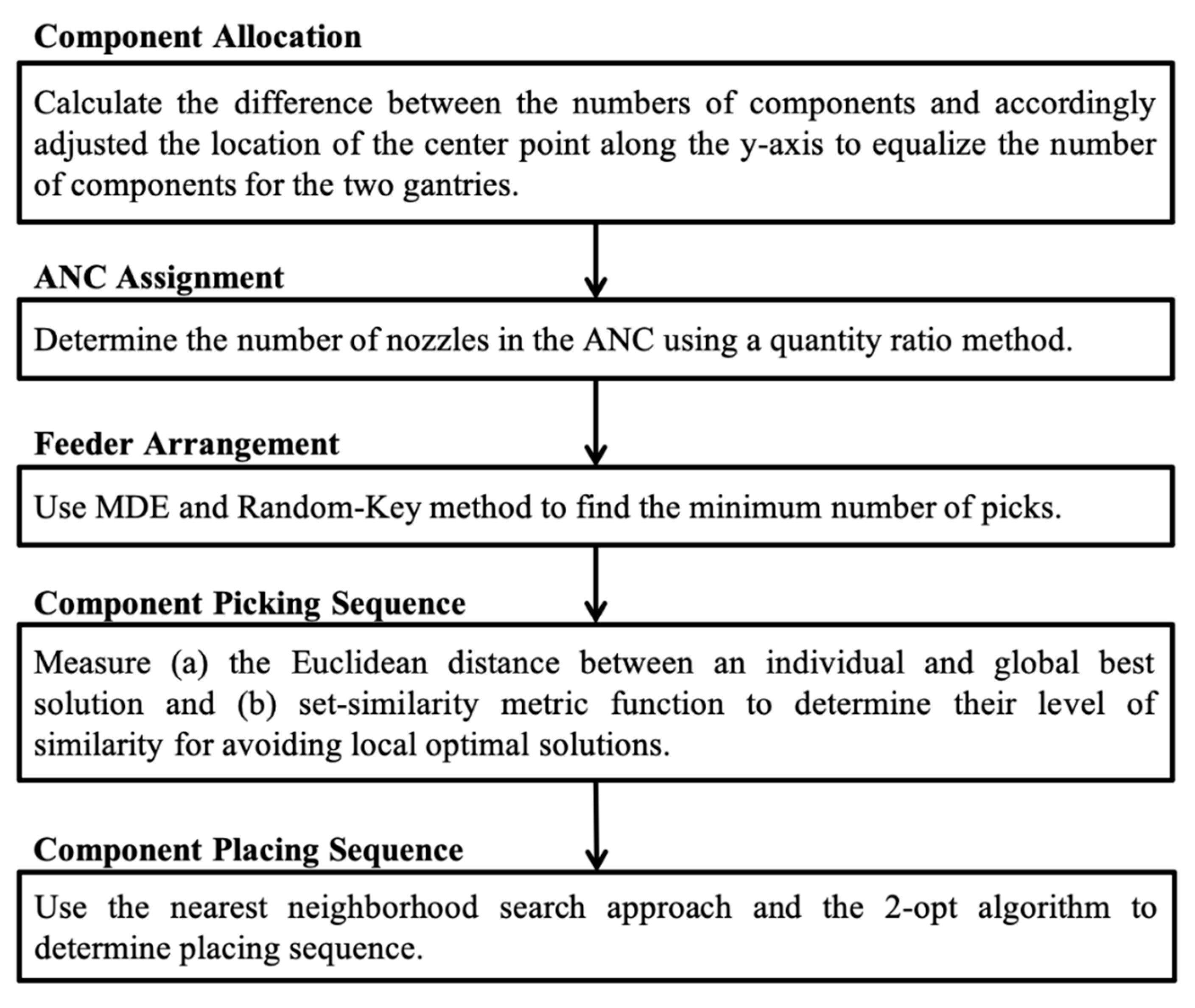The fourth step involves using the nearest-neighbor search approach to determine a tentative placing sequence, which is subsequently planned by the 2-opt method.

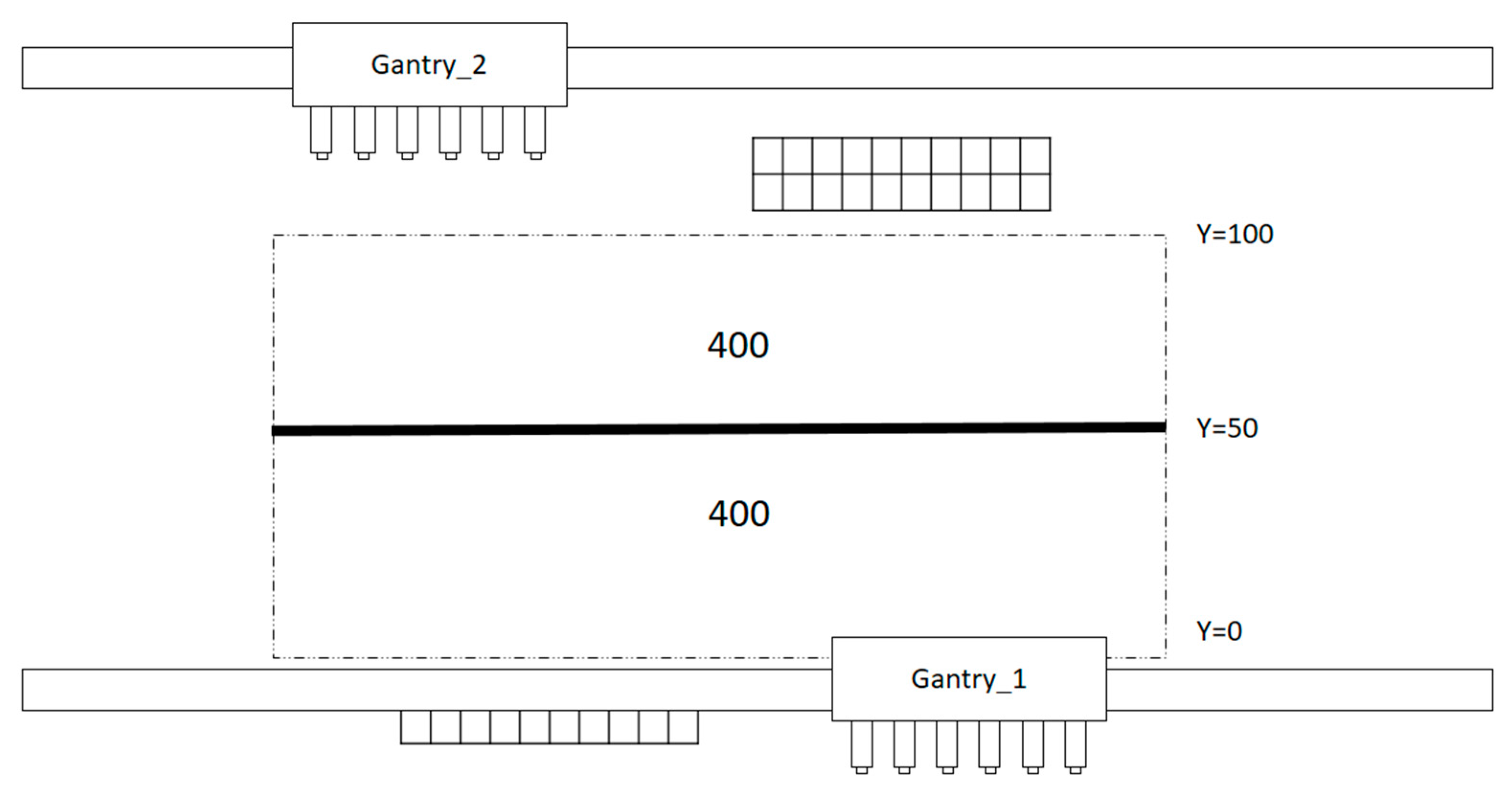
4.1. Component Allocation

The first problem encountered by dual-gantry, multi-head SMP machines is component allocation. Because a gantry cannot pick components from the other gantry’s feeder slots, achieving a component allocation solution that equalizes workloads for the two gantries is the main focus of this step. This study considers component height restriction, which complicates the component allocation problem.

First, the center point of a PCB on the y-axis was identified, and a horizontal line was drawn, dividing the components into those located in upper and lower areas of the PCB board. We calculated the difference between the numbers of components located in the two areas and accordingly adjusted the location of the center point along the y-axis to equalize the number of components for the two gantries.

For example, as presented in Figure 6, when equally dividing the PCB into two halves (Y = 50), both the upper and lower areas each contained 400 components. Gantry_1 was responsible for components in the lower area, and Gantry_2 was responsible for those in the upper area.

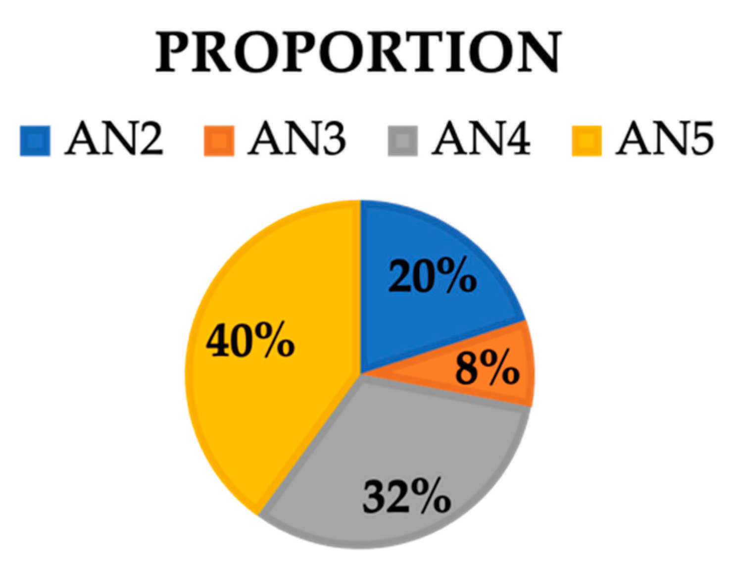
4.2. ANC Assignment Using a Quantity Ratio Method

The number and type of nozzles in the ANC were determined before scheduling. The ANC only have 20 seats: 4 of them are for large nozzles, and 16 are for small nozzles.

According to the number of each type of component to be placed on a PCB, this study used a quantity ratio method to determine the required number for each type of nozzle to be installed at each ANC.

• Step 1:

The number of each type of nozzle is presented in

Table 2. The number of each type of nozzle.

Component		Nozzle		Total Number of Components for the Nozzle	Quantity Ratio
Type	Quantity	Type	Size
D	15	AN2	Small	50	20%
B	35
A	20	AN3	Small	20	8%
E	80	AN4	Small	80	32%
C	100	AN5	Small	100	40%
F	10	ANV1	Large	10	100%

. Four small nozzles (AN2, An3, AN4, and AN5) and one large nozzle (ANV1) are used in this example. Nozzle AN2 picks and places component types D and B; Nozzle AN3 picks and places component type A; Nozzle AN4 picks and places component type E; Nozzle AN5 picks and places component type C; Nozzle ANV1 picks and places component type F. A proportional pie chart (Figure 7) depicts the quantity ratios of the various types of small nozzles. The quantity ratio for each nozzle is calculated as (total number of components for the nozzle) divided by (total number of components for the same size of nozzle). For example, the total number of components for small nozzle is 50 + 20 + 80 + 100 = 250. The quantity ratio for AN2 is equal to 50/250 = 20%.

• Step 2:

To ensure that the gantries can pick up all types of components, the ANC was assigned with at least one seat for each nozzle type (Figure 8).

• Step 3:

Assign nozzles to the remaining seats in ANC according to the predetermined proportions. The calculated values are rounded to the nearest integers. For example, the calculated value for nozzle AN2 is 2.4, and we round it to 2. It means 2 more seats are assigned for nozzle AN2 in ANC. The other seats calculated for nozzles An3, AN4, and AN5 are as follows.

$$AN2:12\times 0.2=2.4 \left(\mathrm{round} \mathrm{to} 2\right),AN3:12\times 0.08=0.96 \left(\mathrm{round} \mathrm{to} 1\right)$$

$$AN4:12\times 0.32=3.84 \left(\mathrm{round} \mathrm{to} 4\right),AN5:12\times 0.4=4.8 \left(\mathrm{round} \mathrm{to} 5\right)$$

There is one more seat for nozzle AN3; 4 more seats for nozzle AN4; and 5 more seats for nozzle AN5. Since there is only one large nozzle used in this example, the four seats for large nozzle are all assigned for ANV1. The final nozzle assignment in ANC was presented in Figure 9.

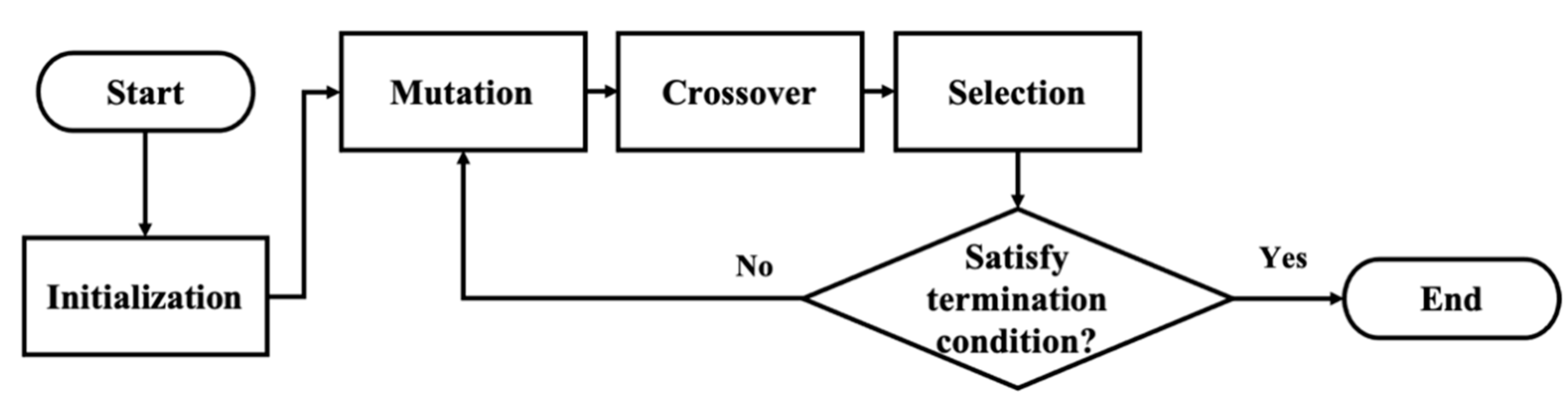
4.3. Feeder Arrangement Using the MDE Algorithm

Evolutionary algorithms are inspired by natural phenomena, biological processes, and human and social behaviors and are widely used to solve scientific and engineering problems because of their simplicity and sensitivity. These algorithms have evolved to be applied in various existing algorithms, such as the genetic algorithm (GA) [10,11,12], particle swarm optimization (PSO) [13,14], and ant colony optimization [15]. The differential evolution (DE) algorithm was first developed by Storn and Price [16,17] in 1995. It is a population-based stochastic optimization algorithm which provides characteristics of simplicity, efficiency, and real coding. The optimization process is conducted through continuous mutation, crossover, and selection until converging to the optimized solution. The flow chart of DE is presented in Figure 10. To optimize the operation of dual-gantry multi-head SMP machines, the following section introduces problems, inter-relationships of problems, and their influences on SMP operations.

(a)

Initialization

The DE algorithm is similar to common heuristic algorithms. Such algorithms begin by initializing individuals and then generating NP individuals randomly in the solution search space. Subsequently, because individuals in a DE algorithm are real numbers, this study obtained random real numbers in the solution search space for each individual. The equation is presented as follows:

$$X_{i,G}^j=X_{min}+rand\left[0,1\right]\ast \left(X_{min}+X_{max}\right)$$

(6)

In this equation, X_min denotes the minimum value, and X_max denotes the maximum value in a solution search space, and $rand \left[0,1\right]$ is a randomly selected real number between 0 and 1. Variable $i$ (individual) represented the place of an individual in an order ($i=0\cdots NP$); G (generation) is the number of generations ($G=0\cdots G_{max}$); and j (dimension) is the size of the dimension ($j=0\cdots D$).

(b)

Mutation

A mutation vector is obtained by calculating the vector difference between individuals, followed by referencing the vector of another individual and a scale factor. For example, randomly pick three individuals, $X_{r1,G}$, $X_{r1,G}$, and $X_{r3,G}$, and then calculate the vector difference between $X_{r2,G}$ and $X_{r3,G}$. Multiply this result by the scale factor, and subsequently add $X_{r1,G}$ to obtain the mutation vector, $V_{i,G+1}$. The equation is presented as follows:

$$V_{i,G+1}^j=X_{r1,G}^j+F\left(X_{r2,G}^j-X_{r3,G}^j\right)$$

(7)

where $r1$, $r2$, and $r3$ are different individuals required for determining the mutation equation, and $r1\ne r2\ne r3$. F is the scale factor. The 2D descript of mutation is shown in Figure 11. The purpose of this study was to optimize the operation of dual-gantry, multi-head SMP machines. The following section introduces problems, inter-relationships of problems, and their influences on SMP operations.

$$U_{i,G+1}^j=\{\begin{array}{c}{V}_{i,G+1}^j,ifran{d}_j\left(0,1\right)\le CR\\ X_{i,G}^j,otherwise\end{array}$$

(8)

where $U_{i,G+1}^j$ is an individual after crossover, $V_{i,G+1}^j$ is a mutated individual, and $X_{i,G}^j$ is the individual before mutation. Regarding the CR ranges of [0,1], a lower CR indicates a smaller effect in enhancing mutation; by contrast, a higher CR implies a stronger effect in enhancing mutation. 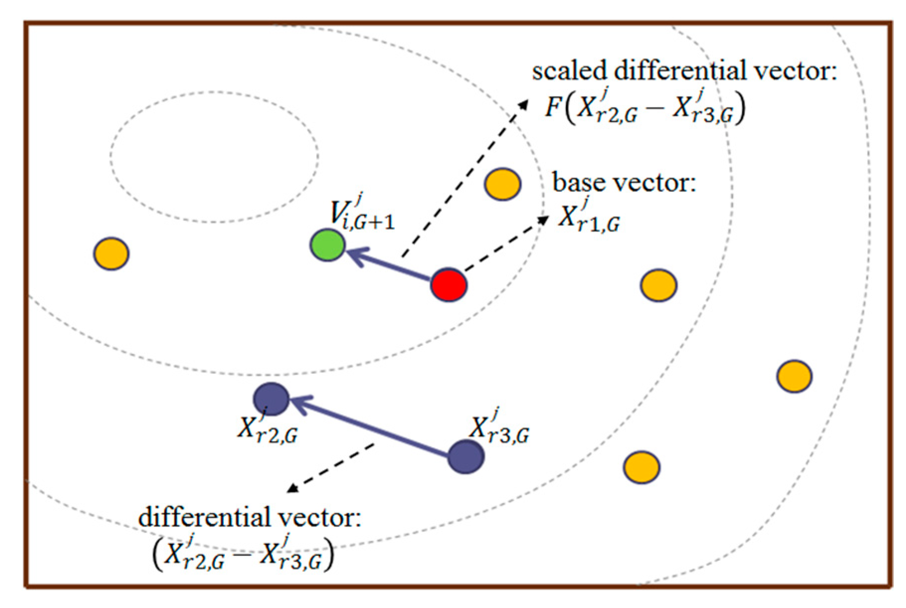Most researchers have suggested that a CR range of [0.8,1] is most effective for a seeking solution.

(c)

Selection

Selection is the final step in a DE algorithm, which evaluates the fitness value of each individual after crossover. After comparing the individuals before and after crossover, which is exhibited, the higher fitness value is used for the next generation of evolution. The equation is presented as follows:

$$X_{i,G+1}=\{\begin{array}{c}{U}_{i,G+1},if Fit\left(U_{i,G+1}\right)>Fit\left(X_{i,G}\right)\\ X_{i,G},otherwise\end{array}$$

(9)

MDE Algorithm

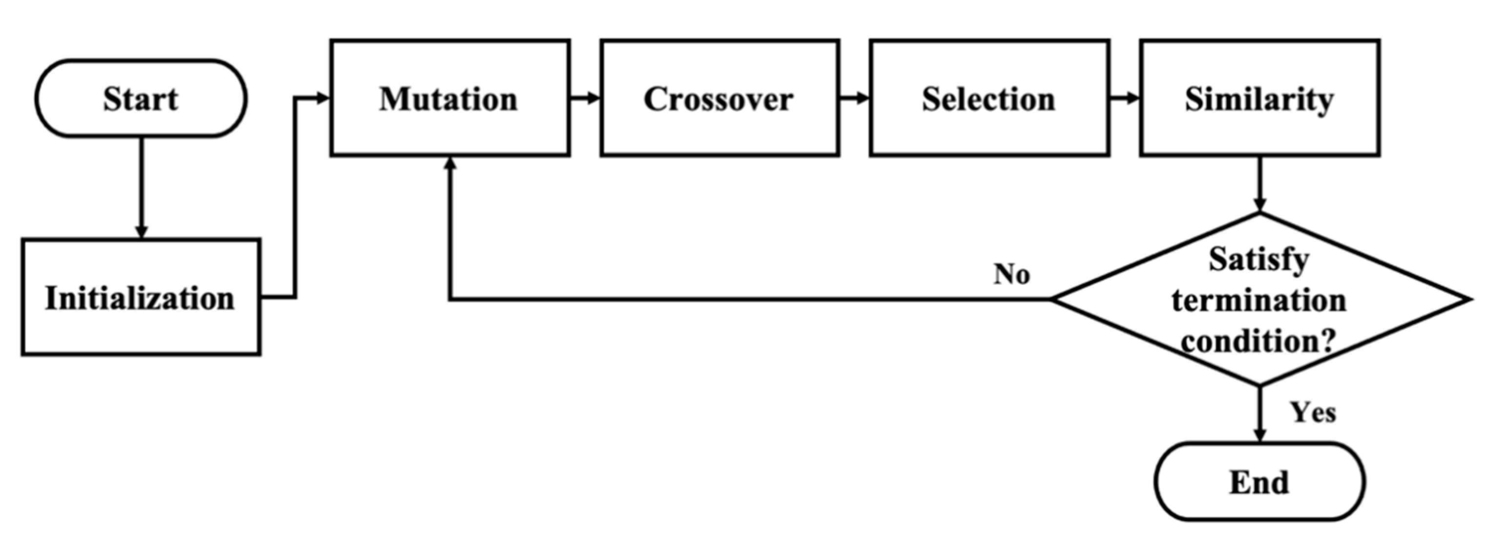
This study chose a DE algorithm and a random-key encoding mapping method for feeder arrangement; however, conventional DE algorithm is often trapped in local solutions owing to its premature convergence. Many researchers have developed new methods for DE to ameliorate the premature convergence. For instance, Choi and Ahn [18] improved DE by monitoring the evolutionary progress of each individual and assigned two control parameters according to the evolution result. Choi and Lee [19] proposed an ex-tended self-adaptive differential evolution algorithm which increases the greediness of jDE algorithm searchability. Choi et al. [20] developed a sigmoid-based parameter control in order to alternate the failure threshold for performing the Cauchy mutation. In this case, the proposed algorithm, which advances the Cauchy mutation, can establish a good ratio between exploration and exploitation. Therefore, instead of monitoring the failure evolution individuals, an MDE algorithm which focuses on expanding the diversity of evolution individuals is proposed in this study. MDE aims to retain the diversity of DE algorithms via removing individuals with high similarity so that the algorithm has more of a chance to search for the optimal solutions. In other words, two similarity measurement mechanisms are introduced to ensure the diversity populations in MDE; therefore, the populations are able to expand the search space. The fitness values of picking sequences were evaluated to derive the least number of picks and picking cycles. The flow chart for MDE algorithm is presented in Figure 12.

(a)

Initialization

The initialization process adopted Equation (6) and the range [0,1] to generate individuals, specifically, $X_{min}$ = 0 and $X_{max}$ = 1.

(b)

Selection

In the calculation of fitness values, the random-key method was used to map the real numbers to integers, each of which represents the index of a feeder slot. The numbers of picks were employed as the fitness values.

Because integers are used for feeder slots, the conventional DE algorithm cannot be adopted directly. The random-key method [21,22] is used to map real numbers to integers. This technique was also applied in this study for mapping the real number of DE individuals to integers, which were subsequently used to number feeder slots.

The random-key method involves mapping real numbers to integers in ascending order. As presented in Figure 13, if an individual’s values are {0.17, 0.51, 0.32, 0.12, 0.35, 0.42}, sorting the real numbers from low to high and assigning an index to each, starting with 1 and indexing by 1 for each successive number, then the mapped integers range from 1 to 6, yielding a mapped result of {2, 6, 3, 1, 4, 5}.

On the basis of the integers determined from the random-key method, components were distributed to their corresponding feeder slots, as presented in Figure 14. Assuming that the feeder slot station has 20 slots and there are 10 components, the first 10 random-keys were selected as slot seats for 10 components.

After components were allocated to feeder slots, the least number of picks was adopted as the reference for picking sequence for each picking cycle. Before the picking process, component heights were examined to ensure they did not exceed the current height restriction. Shorter components must be picked up and placed first to avoid collisions among heads during operation.

(c)

Similarity

Conventional DE algorithms cannot be used to avoid local solutions, which impede the identification of the optimal solution. Therefore, this study applied two similarity methods, measuring the level of similarity between the global best solution ($Gbest$) and others. When multiple individuals are similar to the $Gbest$ position, half of the individuals with inferior fitness values are eliminated and then generate possible offspring to increase the diversity. The remaining individuals are used in the local search to seek more favorable solutions.

This study proposed two similarity measurement mechanisms, both of which use the $Gbest$ position as the measurement criterion and measure its similarity with other individuals.

• Similarity 1: This method measured the Euclidean distance between an individual and $Gbest$ to determine their level of similarity. The mean level of similarity ($Av{g}_{Similarity}$) is the threshold value; individuals with levels of similarity lower than this value are defined as being similar to the $Gbest$ position. The equation is presented as follows:

  $$Similarity1={\displaystyle \sum }_{i=1}^{NP}{\displaystyle \sum }_{j=1}^D\sqrt{{\left(Gbes{t}_j-X_{i,j}\right)}^2}$$

  (10)

  $$Av{g}_{Similarity1}=\frac{Similarity1}{NP}$$

  (11)

  where variable NP is the total number of individuals, D represents dimensions, $Gbes{t}_j$ is the $Gbest$ position, and $X_{i,j}$ represents individual j.
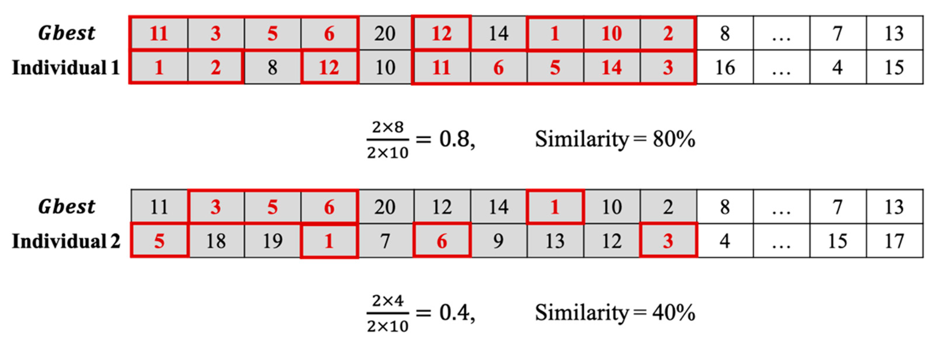
• Similarity 2: Based on the Dice coefficient [23], feeder slots loaded with components are presented in sets to obtain a set-similarity metric function. The equation is presented as follows:

  $$Similarity2=\frac{2\left\{X\cap Y\right\}}{\left\{X\right\}+\left\{Y\right\}}$$

  (12)

  where {X} represents set X, {Y} represents set Y, and $\left\{X\cap Y\right\}$ is the intersection of sets X and Y.

As presented in Figure 15, it is assumed that 20 feeder slots are allocated for 10 components and that only feeder slots to which components have been allocated are counted. This example used the first 10 dimensions as the reference for sets. The set of $Gbest$ position was {11, 3, 5, 6, 20, 12, 14, 1, 10, 2}, the set of Individual 1 was {1, 2, 8, 12, 10, 11, 6, 5, 14, 3}, and the set of Individual 2 was {5, 18, 19, 1, 7, 6, 9, 13, 12, 3}. Those with red grids denote the intersections between them; specifically, $\left|Gbest\cap individual1\right|$ = {1, 2, 3, 5, 6, 11, 12, 14}, and $\left|Gbest\cap individual2\right|$ = {1, 3, 5, 6}. The results of the set metric function on levels of similarity revealed that the similarity of Individual 1 with $Gbest$ was 80%, and the similarity of Individual 2 with $Gbest$ was 40%.

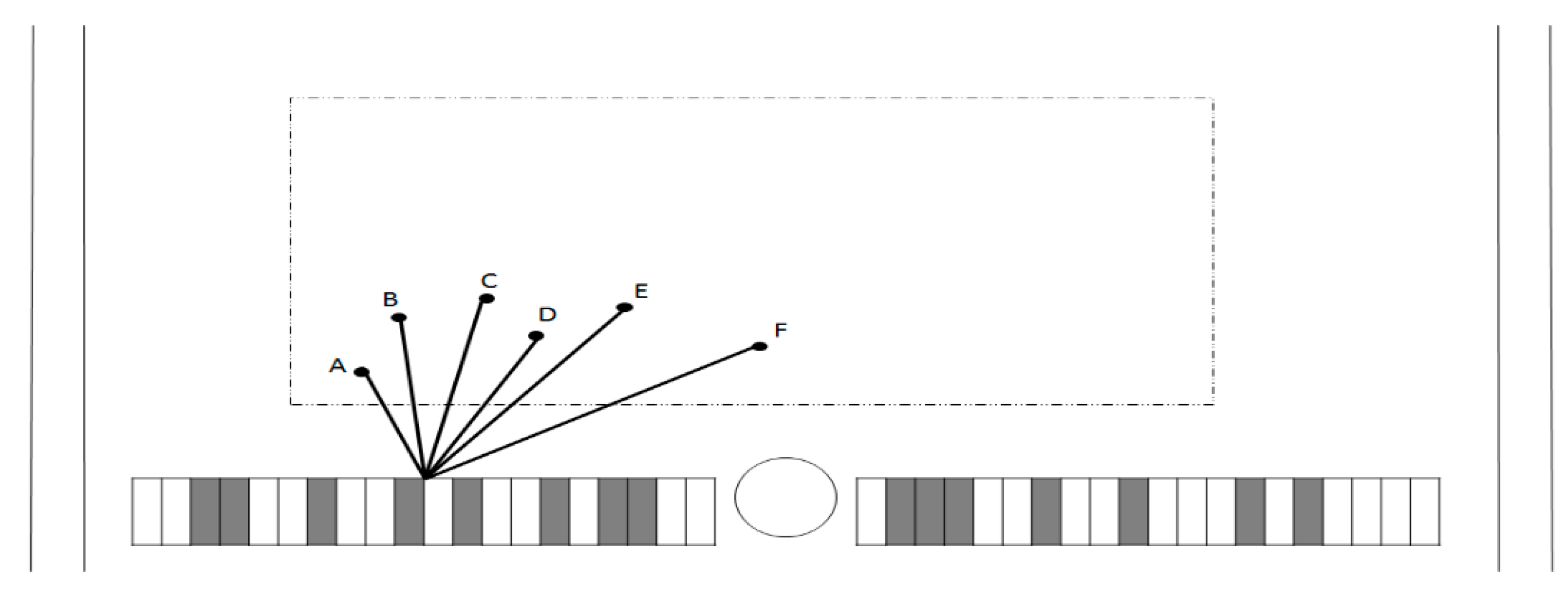
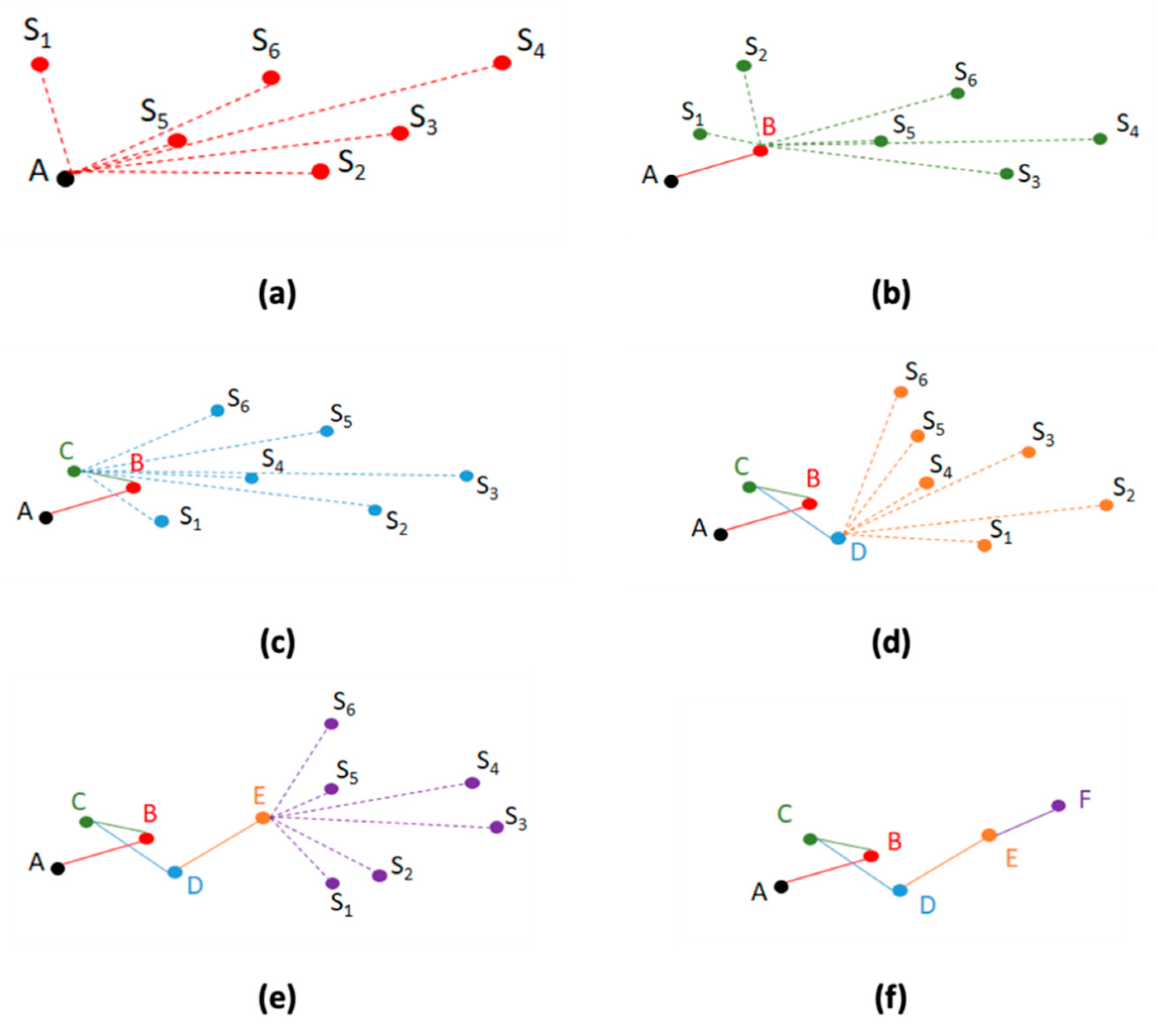
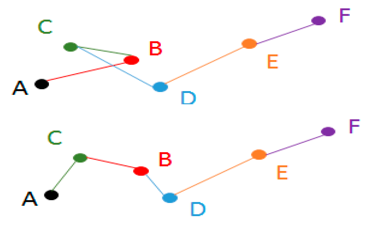
4.4. Determining Placing Sequence Using the Nearest-Neighbor Search and 2-Opt Method

Some heuristics have been studied for solving component-to-feeder assignment and component placing sequence problem. Heuristics such as nearest-neighbor search, nearest insertion, furthest insertion, and random generation were used to initialize a placing sequence. On the other hand, methods such as 2-opt, 3-opt, and Or-opt were used to improve the initial placing sequence [24]. There are many other mathematical optimization approaches for solving the placing sequence problem; however, providing a fast and simple algorithm is better for industrial implementation. Therefore, in this study, a nearest-neighbor search was applied to determine the shortest route for placement; subsequently, the placing routes were shortened by using the 2-opt method. Firstly, component 1 is placed by calculating the distance between the feeder slot and the first placing position. Then, the distance between the first placing position and the second placing position is calculated for component 2. Continue the above steps for all components that need to be placed on a cycle.

The shortest route between a feeder slot and the first component placing position of each cycle is determined independently because each component can be placed in more than one position. We used an example to illustrate how to determine the first placing position. As presented in Figure 16, it is assumed that the first component can be placed in one of the six possible positions, A, B, C, D, E, or F. Using the Euclidean distance to calculate the nearest position from the feeder slot revealed that A is the nearest position, that is, the first component placing position.

Based on the first component placing position, the nearest-neighbor search approach was used to identify the second component placing position, until the placing sequences of all components were determined in Figure 17. Figure 17a shows that the possible second component placing positions are S1–S6, and the nearest distance from the first component placing position A is S2. Therefore, S2 in Figure 17a is selected as the second placing position B. Figure 17b shows that the possible third component placing positions are S1–S6, and the nearest distance from the first component placing position B is S1. Therefore, S1 in Figure 17b is selected as the second placing position C. Continue the selecting process until all the placing positions are determined (Figure 17c–f).

After all placing sequences were obtained, the 2-opt method was used to optimize the route for these placing sequences of all cycles. As presented in Figure 18, the sequence on the top is ABCDEF, which was changed to the sequence on the bottom, ACBDEF, by changing the order of placing sequences C and B.

5. Experimental Results

To verify that the proposed methods are able to reduce the number of picks and shorten the assembly time, this study experimented on 10 PCBs with different numbers and types of components and examined the results. The description of the practical PCBs is presented in

Table 3. PCB information.

PCB	Number of Components	Component Types	Nozzle Types
PCB-1	322	17	5
PCB-2	396	14	4
PCB-3	532	14	4
PCB-4	586	16	3
PCB-5	614	17	2
PCB-6	638	18	4
PCB-7	682	19	5
PCB-8	696	17	5
PCB-9	720	15	3
PCB-10	796	17	2

, and according to the literature reviews [1,2,3,4,5,6,7,8,9], three well-known algorithms including DE, PSO, and GA are compared with the proposed MDE algorithm under the same conditions, and the experimental results are presented in

Table 4. Number of picks.

Methods	MDE				DE		PSO		GA
	Similarity1		Similarity2
Gantry	1	2	1	2	1	2	1	2	1	2
PCB-1	44	61	51	68	62	70	67	75	64	77
PCB-2	47	70	52	64	67	89	89	96	82	87
PCB-3	93	91	92	92	98	94	100	108	96	119
PCB-4	85	73	83	74	103	96	113	90	116	117
PCB-5	106	100	99	100	118	114	119	116	128	124
PCB-6	92	93	95	93	100	107	128	113	127	129
PCB-7	121	128	132	129	142	154	126	159	172	157
PCB-8	108	112	109	117	134	120	130	151	142	151
PCB-9	93	109	94	107	127	117	134	122	129	132
PCB-10	119	124	119	122	141	151	154	137	155	155
Average	90.8	96.1	92.6	96.6	109.2	111.2	116	116.7	121.1	124.8

,

Table 5. The difference of the number of picks.

	DE		PSO		GA
Gantry	1	2	1	2	1	2
MDE Similarity1	−20.3%	−15.7%	−27.7%	−21.4%	−33.4%	−30.0%
MDE Similarity2	−18.0%	−15.1%	−25.2%	−20.8%	−25.3%	−29.2%

,

Table 6. Moving distance for picking.

PCB Methods		PCB-1	PCB-2	PCB-3	PCB-4	PCB-5	PCB-6	PCB-7	PCB-8	PCB-9	PCB-10	Average
MDE Similarity 1	Gantry_1	5535.9	6386.0	14,393.6	13,189.3	7890.4	5687.5	14,087.7	5921.0	14,087.7	8882.6	9606.2
	Gantry_2	22,098.5	24,283.0	35,681.5	38,810.7	45,165.2	53,235.6	52,695.1	49,152.5	52,695.1	51,267.8	42,508.5
MDE Similarity 2	Gantry_1	8996.7	6243.4	8045.6	4909.0	27,345.5	14,804.7	14,339.6	15,061.7	14,339.6	12,437.5	12,652.3
	Gantry_2	28,887.4	24,629.2	36,614.3	38,195.4	45,436.8	43,432.9	52,207.5	58,298.6	52,207.5	52,018.6	43,192.8
DE	Gantry_1	17,300.6	8164.9	17,093.5	18,870.2	16,074.5	20,976.4	29,878.2	16,623.0	29,878.2	22,145.1	19,700.5
	Gantry_2	30,402.3	29,038.3	47,589.3	49,700.0	73,724.1	61,888.1	48,086.1	60,670.6	48,086.1	65,426.5	51,461.1
PSO	Gantry_1	20,085.0	46,903.4	14,901.8	19,732.4	50,936.9	56,762.9	30,744.5	76,028.7	30,744.5	62,205.5	40,904.6
	Gantry_2	26,791.4	65,493.1	68,364.6	44,386.8	56,528.2	51,164.0	52,767.6	75,556.7	52,767.6	61,737.6	55,555.8
GA	Gantry_1	15,732.5	31,684.0	21,321.1	55,354.4	55,776.3	76,430.6	25,093.5	26,523.6	25,093.5	26,929.9	35,993.9
	Gantry_2	34,702.8	27,899.8	66,586.1	22,457.9	52,666.3	37,960.3	48,536.2	72,913.3	48,536.2	63,998.6	47,625.8

,

Table 7. Assembly time for each PCB.

Methods PCB	MDE		DE	PSO	GA
	Similarity1	Similarity2
PCB-1	194.1	193.5	211.4	197.5	212.8
PCB-2	277.3	282.8	301.9	324.8	297.2
PCB-3	184.6	179.3	194.7	227.9	233.2
PCB-4	233.8	222.3	242.0	245.7	250.0
PCB-5	287.8	294.3	312.1	321.4	313.6
PCB-6	274.0	284.0	288.3	314.4	313.7
PCB-7	318.5	304.2	373.2	343.3	352.6
PCB-8	245.5	267.4	284.6	284.0	282.1
PCB-9	350.5	349.4	387.1	409.6	361.8
PCB-10	296.5	305.0	329.0	340.6	308.6
Average	266.26	268.22	292.43	300.92	292.56

and

Table 8. The difference of assembly time for each PCB.

	DE	PSO	GA
MDE Similarity1	−9.8%	−13.0%	−9.8%
MDE Similarity2	−9.0%	−12.2%	−9.1%

. The parameter NP was 30, iteration time was 1000, CR was 0.8, and scaling factor was 0.9. Equation (6) was used for mutation calculation.

Table 4 and Table 6 compare the number of picks and moving distance of gantries during their component picking processes, respectively. Those two tables are mainly used to evaluate the feeder arrangement and picking sequence using the proposed MDE algorithm and other algorithms. Table 7 describes the assembly time for each PCB, which is focusing on assessing the performance of placing sequence using the NNS and 2-opt method.

According to Table 4 and Figure 19, MDE is better than DE, DE is better than PSO, and PSO is better than GA. The experimental results can be discussed in light of [25], where the solutions of GA are ranked based on the fitness values and the offspring solutions produced by crossover are more likely to be similar to the parents. In the other words, it is often found that GA operators cannot produce all potential solutions. For PSO, a new swarm of particles is generated via the velocity and position update equations, ensuring that all new particles can be very different than the old ones. Based on this observation, PSO could generate any potential values within the solution space. Since the best particle in the swarm is able to influence all the remaining solutions, this might lead to premature convergence of the population toward a particular solution. Similar to PSO, DE is also based on floating-point arithmetic; however, the diversification of DE is better because the best solution does not influence the other solutions. Moreover, the mutant vector is a solution that is not from the original population.

Nevertheless, to remedy the drawback of the tendency of those three algorithms to rapidly converge, a very frequently used alternative is to keep the global best particle and regenerate all or part of the remaining particles. In this study, the MDE algorithm, which removes populations with high similarity to retain the diversity of the solutions, is presented and the experimental results demonstrate considerably fewer average number of picks than conventional DE, PSO, and GA conducted by Gantry_1 and Gantry_2.

In Figure 19, compared with those three algorithms, the MDE algorithm is able to jump off the local optimal solution with less generations, which may be the reason the two similarity measurement mechanisms are used. In addition, the MDE with Euclidean distance similarity method can converge faster than the similarity method using the Dice coefficient; however, their final results of average number of picks are almost the same. From those experimental results, the MDE algorithm is shown to be the highest performance in feeder arrangement compared with DE, PSO, and GA. Moreover, Table 5 demonstrates the difference of number of picks using MDE in comparison with those of three well-known algorithms. A gantry can reduce at most 30% of the number of picks while using the MDE algorithm which meets the company’s needs, which provided the practical PCB data in this experiment; however, according to no free lunch theorem [26] once the number of components increased in each PCBs (>1000) or the types of components vary (>30), the training time of MDE might increase, which results in time-consuming manufacturing.

Table 6 displayed that the moving distances of two gantries for the picking process were decreased with the proposed MDE algorithm. From Table 4 and Table 6, the results reveal that in comparison to other evolutionary algorithms, the MDE algorithm provides a proper feeder arrangement which is able to reduce the number of picks and also reduce the gantries’ moving distances.

Table 7 presents the total picking-and-placing assembly time required for each of the 10 PCBs. A combination of NNS and 2-opt method is primarily involved in components placing operation. The total assembly time was calculated using Equation (6), which involved comparing the time required by the two gantries to finish their tasks. Figure 20 depicts the assembly of PCB-1 using Similarity 1 in the MDE algorithm as the example. When Gantry_1 was placing components and Gantry_2 was picking components, the longer time required between the two simultaneous operations was used in the calculation. Similarly, when Gantry_1 was picking components and Gantry_2 was placing components, as shown in Figure 21, only the longer time required between the two simultaneous operations was used in the calculation. Finally, the sum of the time represented the total assembly time, as presented in Figure 22. The proposed methods required less assembly time for PCBs tested as shown numerically in Table 7 and graphically in Figure 23. Table 8 demonstrates the difference of assembly time for each PCB using the MDE in comparison with those of the three well-known algorithms. The assembly time is decreased at most by 13% using the proposed method.

6. Conclusions

This study focuses on the component allocation and feeder arrangement for dual-gantry multi-head SMP machines and solves related scheduling problems using four approaches. The component allocation problem was solved using a workload equalizing approach, which equalized component allocation to the two gantries. The ANC assignment problem was solved using quantity ratio method to determine the required number for each type of nozzle to be installed at each ANC. Moreover, the proposed MDE algorithm identifying the picking sequence that gave the least number of picks was applied for the feeder arrangement. The nearest-neighbor search method was used for deriving initial solutions, and then the 2-opt method was applied to improve the tentative placement routes. Experimental results show that the number of picks, moving distance of picking components, and total assembly time with the proposed MDE algorithm are less than those from DE, PSO, and GA algorithms. This study provides a reference for SMP scheduling in PCB industry.

Practically, there are many types of components placed in a PCB, and sometimes the components are not equal in equal size. Larger component size occupies two head spaces, and the adjacent head cannot be used for other components. The restriction of component shape is not considered in the current study, and this can be conducted in the future work. Additional experiments are suggested to consider (i) the effect of components on shape and component orientation, and their impact on picking and placing; and (ii) whether other optimal algorithms such as modified PSO/GA can be implemented in the future to obtain comprehensive results and demonstrate whether the proposed MDE algorithm is superior.

References

- Sun, D.S.; Lee, T.E.; Kim, K.H. Component allocation and feeder arrangement for a dual-gantry multi-head surface mount placement tool. Int. J. Prod. Econ. 2005, 95, 245–264. [Google Scholar] [CrossRef]
- Du, X.; Li, Z. Placement process optimization of dual-gantry turret placement machine. In Proceedings of the 2008 IEEE/ASME International Conference on Advanced Intelligent Mechatronics, Xi’an, China, 2–5 July 2008; pp. 1266–1271. [Google Scholar]
- Ashayeri, J.; Ma, N.; Sotirov, R. An aggregated optimization model for multi-head SMD placements. Comput. Ind. Eng. 2011, 60, 99–105. [Google Scholar] [CrossRef][Green Version]
- Torabi, S.A.; Hamedi, M.; Ashayeri, J. A new optimization approach for nozzle selection and component allocation in multi-head beam-type SMD placement machines. J. Manuf. Syst. 2013, 32, 700–714. [Google Scholar] [CrossRef]
- Zhu, G.-Y.; Zhang, W.-B. An improved Shuffled Frog-leaping Algorithm to optimize component pick-and-place sequencing optimization problem. Expert Syst. Appl. 2014, 41, 6818–6829. [Google Scholar] [CrossRef]
- He, T.; Li, D.; Yoon, S.W. A Hierarchical Restricted Balance Approach for Workload Balance of a Dual-Delivery SMT Placement Machine. In Proceedings of the IIE Annual Conference, Nashville, TN, USA, 30 May–2 June 2015; pp. 808–817. [Google Scholar]
- Li, D.; Yoon, S.W. PCB assembly optimization in a single gantry high-speed rotary-head collect-and-place machine. Int. J. Adv. Manuf. Technol. 2017, 88, 2819–2834. [Google Scholar] [CrossRef]
- He, T.; Li, D.; Yoon, S.W. A multi-phase planning heuristic for a dual-delivery SMT placement machine optimization. Robot. Comput.-Integr. Manuf. 2017, 47, 85–94. [Google Scholar] [CrossRef]
- Huang, Y.; Zhao, L.; Liu, P. Applied Research of Hierarchical Multi-objective Optimization Method in High Speed and High Precision Placement Machine. J. Phys. Conf. Ser. 2020, 1605, 012029. [Google Scholar] [CrossRef]
- Lin, H.Y.; Lin, C.J.; Huang, M.L. Optimization of printed circuit board component placement using an efficient hybrid genetic Algorithm. Appl. Intell. 2016, 45, 622–637. [Google Scholar] [CrossRef]
- He, T.; Li, D.; Yoon, S.W. An adaptive clustering-based genetic algorithm for the dual-gantry pick-and place machine optimization. Adv. Eng. Inform. 2018, 37, 66–78. [Google Scholar] [CrossRef]
- Li, Z.; Yu, X.; Qiu, J.; Gao, H. Cell Division Genetic Algorithm for Component Allocation Optimization in Multi-Functional Placers. IEEE Trans. Ind. Inform. (Early Access) 2021. [Google Scholar] [CrossRef]
- Huang, X.; Li, C.; Chen, H.; An, D. Task scheduling in cloud computing using particle swarm optimization with time varying inertia weight strategies. Clust. Comput. 2019, 23, 1137–1147. [Google Scholar] [CrossRef]
- Hsu, H.P. Solving feeder assignment and component sequencing problems for printed circuit board assembly using particle swarm optimization. IEEE Trans. Autom. Sci. Eng. 2017, 14, 881–893. [Google Scholar] [CrossRef]
- Zhao, H.; Gao, W.; Deng, W.; Sun, M. Study on an Adaptive Co-Evolutionary ACO Algorithm for Complex Optimization Problems. Symmetry 2018, 10, 104. [Google Scholar] [CrossRef]
- Storn, R. On the usage of differential evolution for function optimization. In Proceedings of the Biennial Conference of the North American Fuzzy Information Processing Society (NAFIPS), Berkeley, CA, USA, 19–22 June 1996; pp. 519–523. [Google Scholar]
- Storn, R.; Price, K. Differential evolution—A simple and efficient adaptive scheme for global optimization over continuous spaces. J. Glob. Optim. 1997, 11, 341–359. [Google Scholar] [CrossRef]
- Choi, T.J.; Ahn, C.W. An Improved Differential Evolution Algorithm and Its Application to Large-Scale Artificial Neural Networks. J. Phys. Conf. Ser. 2017, 806, 012010. [Google Scholar] [CrossRef]
- Choi, T.J.; Lee, Y. Asynchronous differential evolution with self- adaptive parameter control for global numerical optimization. Matec Web Conf. 2018, 189, 03020. [Google Scholar] [CrossRef]
- Choi, T.J.; Togelius, J.; Cheong, Y.-G. Advanced Cauchy Mutation for Differential Evolution in Numerical Optimization. IEEE Access 2020, 8, 8720–8734. [Google Scholar] [CrossRef]
- Bean, J.C. Genetic Algorithms and Random Keys for Sequencing and Optimization. INFORMS J. Comput. 1994, 6, 154–160. [Google Scholar] [CrossRef]
- Faria, H.; Resende, M.G.; Ernst, D. A biased random key genetic algorithm applied to the electric distribution network reconfiguration problem. J. Heuristics 2017, 23, 533–550. [Google Scholar] [CrossRef]
- Dice, L.R. Measures of the Amount of Ecologic Association Between Species. Ecology 1945, 26, 297–302. [Google Scholar] [CrossRef]
- Hsu, H.-P. Printed Circuit Board Assembly Planning for Multi-Head Gantry SMT Machine Using Multi-Swarm and Discrete Firefly Algorithm. IEEE Access 2020, 9, 1642–1654. [Google Scholar] [CrossRef]
- Kachitvichyanukul, V. Comparison of Three Evolutionary Algorithms: GA, PSO, and DE. Ind. Eng. Manag. Syst. 2012, 11, 215–223. [Google Scholar] [CrossRef]
- Wolpert, D.H.; Macready, W.G. No free lunch theorems for optimization. IEEE Trans. Evol. Comput. 1997, 1, 67–82. [Google Scholar] [CrossRef]