
Logistic Biplot by Conjugate Gradient Algorithms and Iterated SVD


Abstract
1. Introduction
2. Materials and Methods
2.1. Biplot for Continuous Data
2.2. Logistic Biplot
2.3. Parameter Estimation
2.3.1. Estimation Using Nonlinear Conjugate Gradient Algorithms
| Algorithm 1 CG Algorithm for fitting a LB model |
| Input |
| Output |
| 1: Initialize |
| 2: |
| 3: |
| 4: |
| 5: l = 0 |
| 6: repeat |
| 7: |
| 8: |
| 9: |
| 10: |
| 11: |
| 12: |
| 13: |
| 14: Compute according to one of the formulas given in (13) |
| 15: |
| 16: until |
2.3.2. Estimation Using Coordinate Descendent MM Algorithm
| Algorithm 2 Coordinate descendent MM algorithm for fitting a LB model |
| Input |
| Output |
| 1: Initialize |
| 2: |
| 3: l = 0 |
| 4: repeat |
| 5: |
| 6: |
| 7: |
| 8: , with |
| 9: |
| 10: |
| 11: |
| 12: |
| 13: until |
2.4. Simulated and Real Data
2.4.1. Real Data
2.4.2. Simulation Process
| Algorithm 3 Algorithm to simulate a binary data matrix |
| Input . |
| Output |
| 1: with . |
| 2: procedure Gram–Schmidt algorithm |
| 3: |
| 4: end procedure |
| 5: with |
| 6: |
| 7: |
| 8: , with . |
2.5. Model Performance Assessment
3. Results
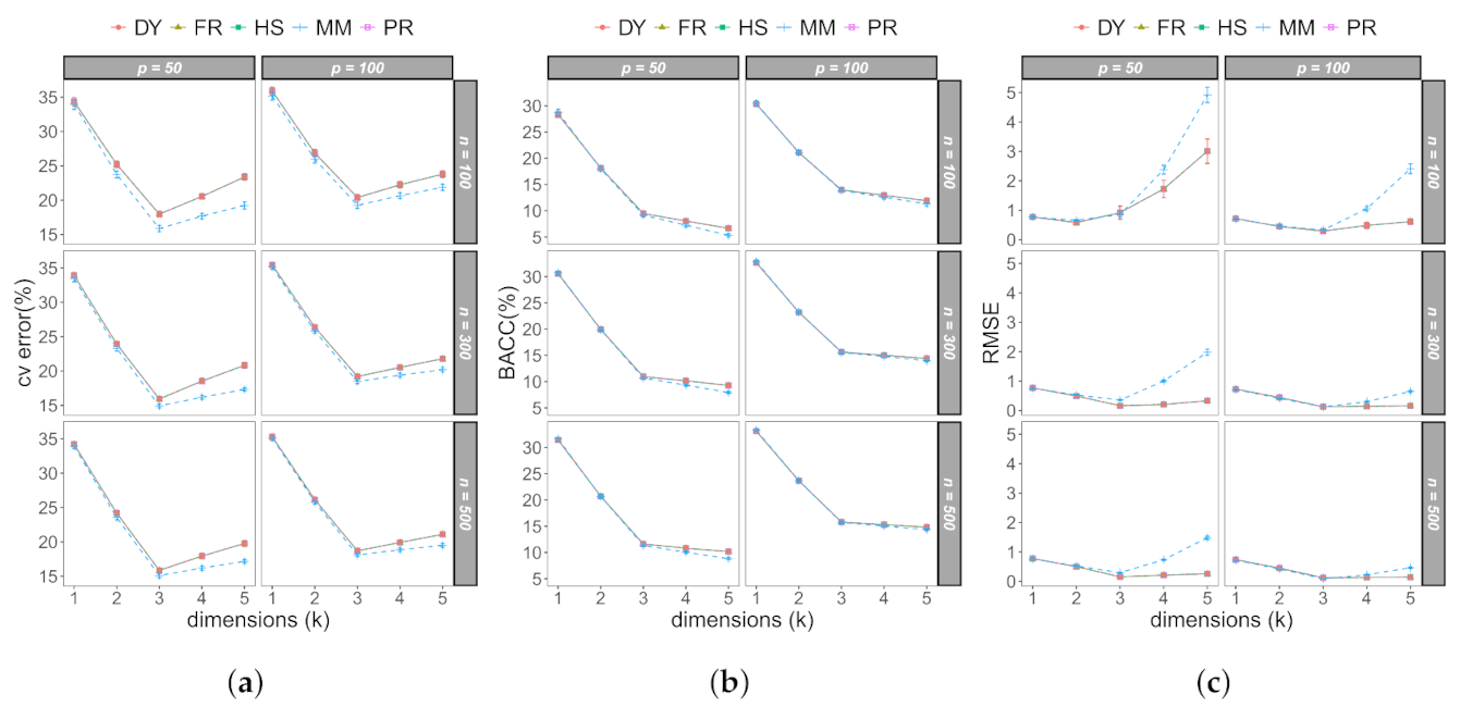
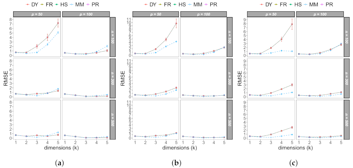
3.1. Monte Carlo Study
3.2. Application
4. Conclusions and Discussion
Author Contributions
Funding
Institutional Review Board Statement
Informed Consent Statement
Data Availability Statement
Conflicts of Interest
Abbreviations
| LB | Logistic Biplot |
| MM | Majorization–Minimization |
| CG | Conjugate Gradient |
| PCA | Principal Component Analysis |
| BACC | Balanced Accuracy |
| RMSE | Relative Mean Squared Error |
| SVD | Singular Value Decomposition |
| NIPALS | Nonlinear estimation by Iterative Partial Least Square |
| LTA | Latent Trait Analysis |
| IRT | Item Response Theory |
| RE-WLR | Rare Event Weighted Logistic Regression |
| TR-IRLS | Truncated Regularized Iteratively Re-weighted Least Squares |
Appendix A. Derivatives
References
- Keller, K. Strategic Brand Management: Building, Measuring, and Managing Brand Equity; Pearson/Prentice Hall: Hoboken, NJ, USA, 2008. [Google Scholar]
- Murray, D.; Pals, S.; Blitstein, J. Design and Analysis of Group-Randomized Trials: A Review of Recent Methodological Developments. Am. J. Public Health 2004, 94, 423–432. [Google Scholar] [CrossRef]
- Moerbeek, M.; Breukelen, G.; Berger, M. Optimal Experimental Designs for Multilevel Logistic Models. J. R. Stat. Soc. Ser. D Stat. 2001, 50, 17–30. [Google Scholar] [CrossRef]
- Moerbeek, M.; Maas, C. Optimal Experimental Designs for Multilevel Logistic Models with Two Binary Predictors. Commun. Stat. Theory Methods 2005, 34. [Google Scholar] [CrossRef]
- Iorio, F.; Knijnenburg, T.A.; Vis, D.J.; Bignell, G.R.; Menden, M.P.; Schubert, M.; Aben, N.; Gonçalves, E.; Barthorpe, S.; Lightfoot, H.; et al. A landscape of pharmacogenomic interactions in cancer. Cell 2016, 166, 740–754. [Google Scholar] [CrossRef] [PubMed]
- Collins, M.; Dasgupta, S.; Schapire, R.E. A generalization of principal components analysis to the exponential family. In Advances in Neural Information Processing Systems 14; The MIT Press: Cambridge, MA, USA, 2001; pp. 617–624. [Google Scholar]
- Schein, A.I.; Saul, L.K.; Ungar, L.H. A Generalized Linear Model for Principal Component Analysis of Binary Data. In Proceedings of the 9th International Workshop on Artificial Intelligence and Statistics, Key West, FL, USA, 3–6 January 2003; Volume 38. [Google Scholar]
- De Leeuw, J. Principal component analysis of binary data by iterated singular value decomposition. Comput. Stat. Data Anal. 2006, 50, 21–39. [Google Scholar] [CrossRef]
- Lee, S.; Huang, J.Z.; Hu, J. Sparse logistic principal components analysis for binary data. Ann. Appl. Stat. 2010, 4, 1579–1601. [Google Scholar] [CrossRef]
- Lee, S.; Huang, J. A coordinate descent MM algorithm for fast computation of sparse logistic PCA. Comput. Stat. Data Anal. 2013, 62, 26–38. [Google Scholar] [CrossRef]
- Landgraf, A.J.; Lee, Y. Dimensionality reduction for binary data through the projection of natural parameters. J. Multivar. Anal. 2020, 180, 104668. [Google Scholar] [CrossRef]
- Song, Y.; Westerhuis, J.A.; Smilde, A.K. Logistic principal component analysis via non-convex singular value thresholding. Chemom. Intell. Lab. Syst. 2020, 204, 104089. [Google Scholar] [CrossRef]
- Gabriel, K.R. The biplot graphic display of matrices with application to principal component analysis 1. Biometrika 1971, 58, 453–467. [Google Scholar] [CrossRef]
- Gower, J.C.; Lubbe, S.G.; Le Roux, N.J. Understanding Biplots; John Wiley and Sons: Hoboken, NJ, USA, 2011. [Google Scholar]
- Scrucca, L. Graphical tools for model-based mixture discriminant analysis. Adv. Data Anal. Classif. 2014, 8, 147–165. [Google Scholar] [CrossRef]
- Groenen, P.J.; Le Roux, N.J.; Gardner-Lubbe, S. Spline-based nonlinear biplots. Adv. Data Anal. Classif. 2015, 9, 219–238. [Google Scholar] [CrossRef]
- Kendal, E.; Sayar, M. The stability of some spring triticale genotypes using biplot analysis. J. Anim. Plant Sci. 2016, 26, 754–765. [Google Scholar]
- Amor-Esteban, V.; Galindo-Villardón, M.P.; García-Sánchez, I.M. A multivariate proposal for a national corporate social responsibility practices index (NCSRPI) for international settings. Soc. Indic. Res. 2019, 143, 525–560. [Google Scholar] [CrossRef]
- González-García, N.; Nieto-Librero, A.B.; Vital, A.L.; Tao, H.J.; González-Tablas, M.; Otero, Á.; Galindo-Villardón, P.; Orfao, A.; Tabernero, M.D. Multivariate analysis reveals differentially expressed genes among distinct subtypes of diffuse astrocytic gliomas: Diagnostic implications. Sci. Rep. 2020, 10, 1–12. [Google Scholar] [CrossRef]
- Galindo Villardón, M.P. Una alternativa de representación simultánea: HJ-Biplot. Questiio 1986, 10, 13–23. [Google Scholar]
- Gower, J.C.; Hand, D.J. Biplots; CRC Press: Boca Raton, FL, USA, 1995; Volume 54. [Google Scholar]
- Greenacre, M.; Blasius, J. Multiple Correspondence Analysis and Related Methods; Chapman and Hall/CRC: London, UK, 2006. [Google Scholar]
- Hernández-Sánchez, J.C.; Vicente-Villardón, J.L. Logistic biplot for nominal data. Adv. Data Anal. Classif. 2017, 11, 307–326. [Google Scholar] [CrossRef][Green Version]
- Cubilla-Montilla, M.; Nieto-Librero, A.B.; Galindo-Villardón, M.P.; Torres-Cubilla, C.A. Sparse HJ Biplot: A New Methodology via Elastic Net. Mathematics 2021, 9, 1298. [Google Scholar] [CrossRef]
- Gabriel, K.R. Generalised Bilinear Regression. Biometrika 1998, 85, 689–700. [Google Scholar] [CrossRef]
- Vicente-Villardon, J.; Galindo-Villardon, M.; Blazquez-Zaballos, A. Logistic Biplots. In Multiple Correspondence Analysis and Related Methods; Chapman-Hall: London, UK, 2006; Chapter 23; pp. 503–521. [Google Scholar]
- Demey, J.; Vicente Villardon, J.L.; Galindo Villardón, M.P.; Zambrano, A. Identifying molecular markers associated with classification of genotypes by External Logistic Biplots. Bioinformatics 2008, 24, 2832–2838. [Google Scholar] [CrossRef] [PubMed]
- Vicente-Villardón, J.L.; Hernández-Sánchez, J.C. External Logistic Biplots for Mixed Types of Data. In Advanced Studies in Classification and Data Science; Springer: New York, NY, USA, 2020; pp. 169–183. [Google Scholar]
- Komarek, P.; Moore, A.W. Fast Robust Logistic Regression for Large Sparse Datasets with Binary Outputs. In Proceedings of the Ninth International Workshop on Artificial Intelligence and Statistics, Key West, FL, USA, 3–6 January 2003; pp. 163–170. [Google Scholar]
- Lewis, J.M.; Lakshmivarahan, S.; Dhall, S. Dynamic Data Assimilation: A Least Squares Approach; Cambridge University Press: Cambridge, UK, 2006; Volume 13. [Google Scholar]
- King, G.; Zeng, L. Logistic Regression in Rare Events Data. Political Anal. 2001, 9, 137–163. [Google Scholar] [CrossRef]
- Maalouf, M.; Siddiqi, M. Weighted logistic regression for large-scale imbalanced and rare events data. Knowl. Based Syst. 2014, 59, 142–148. [Google Scholar] [CrossRef]
- Babativa-Marquez, J.G. Package BiplotML: Biplots Estimation with Machine Learning Algorithms. Available online: https://cran.r-project.org/package=BiplotML (accessed on 24 June 2021).
- R Core Team. R: A Language and Environment for Statistical Computing; R Foundation for Statistical Computing: Vienna, Austria, 2020. [Google Scholar]
- Wold, H. Estimation of principal components and related models by iterative least squares. In Multivariate Analysis; Academic Press: NewYork, NY, USA, 1966; pp. 391–420. [Google Scholar]
- Owen, A.B.; Perry, P.O. Bi-cross-validation of the SVD and the nonnegative matrix factorization. Ann. Appl. Stat. 2009, 3, 564–594. [Google Scholar] [CrossRef]
- Pytlak, R. Conjugate Gradient Algorithms in Nonconvex Optimization; Springer Science & Business Media: Berlin, Germany, 2008; Volume 89. [Google Scholar]
- Nocedal, J.; Wright, S. Numerical Optimization; Springer Science & Business Media: Berlin, Germany, 2006. [Google Scholar]
- Fletcher, R.; Powell, M.J. A rapidly convergent descent method for minimization. Comput. J. 1963, 6, 163–168. [Google Scholar] [CrossRef]
- Polak, E.; Ribiere, G. Note sur la convergence de méthodes de directions conjuguées. ESAIM Math. Model. Numer. Anal. Model. Math. Anal. Numer. 1969, 3, 35–43. [Google Scholar] [CrossRef]
- Polyak, B.T. The conjugate gradient method in extremal problems. USSR Comput. Math. Math. Phys. 1969, 9, 94–112. [Google Scholar] [CrossRef]
- Dai, Y.H.; Yuan, Y. A nonlinear conjugate gradient method with a strong global convergence property. SIAM J. Optim. 1999, 10, 177–182. [Google Scholar] [CrossRef]
- Dai, Y.H.; Yuan, Y. An efficient hybrid conjugate gradient method for unconstrained optimization. Ann. Oper. Res. 2001, 103, 33–47. [Google Scholar] [CrossRef]
- Zhang, L.; Zhou, W.; Li, D.H. A descent modified Polak–Ribière–Polyak conjugate gradient method and its global convergence. IMA J. Numer. Anal. 2006, 26, 629–640. [Google Scholar] [CrossRef]
- Andrei, N. A hybrid conjugate gradient algorithm for unconstrained optimization as a convex combination of Hestenes-Stiefel and Dai-Yuan. Stud. Inform. Control 2008, 17, 57. [Google Scholar]
- Yuan, G.; Zhang, M. A modified Hestenes-Stiefel conjugate gradient algorithm for large-scale optimization. Numer. Funct. Anal. Optim. 2013, 34, 914–937. [Google Scholar] [CrossRef]
- Liu, J.; Li, S. New hybrid conjugate gradient method for unconstrained optimization. Appl. Math. Comput. 2014, 245, 36–43. [Google Scholar] [CrossRef]
- Dong, X.L.; Liu, H.W.; He, Y.B.; Yang, X.M. A modified Hestenes–Stiefel conjugate gradient method with sufficient descent condition and conjugacy condition. J. Comput. Appl. Math. 2015, 281, 239–249. [Google Scholar] [CrossRef]
- Yuan, G.; Wei, Z.; Yang, Y. The global convergence of the Polak–Ribiere–Polyak conjugate gradient algorithm under inexact line search for nonconvex functions. J. Comput. Appl. Math. 2019, 362, 262–275. [Google Scholar] [CrossRef]
- Al-Baali, M. Descent property and global convergence of the Fletcher—Reeves method with inexact line search. IMA J. Numer. Anal. 1985, 5, 121–124. [Google Scholar] [CrossRef]
- Dai, Y.; Yuan, Y.X. Convergence properties of the Fletcher-Reeves method. IMA J. Numer. Anal. 1996, 16, 155–164. [Google Scholar] [CrossRef]
- Kiers, H.A. Weighted least squares fitting using ordinary least squares algorithms. Psychometrika 1997, 62, 251–266. [Google Scholar] [CrossRef]
- Velez, D.R.; White, B.C.; Motsinger, A.A.; Bush, W.S.; Ritchie, M.D.; Williams, S.M.; Moore, J.H. A balanced accuracy function for epistasis modeling in imbalanced datasets using multifactor dimensionality reduction. Genet. Epidemiol. Off. Publ. Int. Genet. Epidemiol. Soc. 2007, 31, 306–315. [Google Scholar] [CrossRef]
- Wei, Q.; Dunbrack, R.L., Jr. The role of balanced training and testing data sets for binary classifiers in bioinformatics. PLoS ONE 2013, 8, e67863. [Google Scholar] [CrossRef]
- Wold, S. Cross-validatory estimation of the number of components in factor and principal components models. Technometrics 1978, 20, 397–405. [Google Scholar] [CrossRef]
- Gabriel, K.R. Le biplot-outil d’exploration de données multidimensionnelles. J. Soc. Fr. Stat. 2002, 143, 5–55. [Google Scholar]
- Bro, R.; Kjeldahl, K.; Smilde, A.K.; Kiers, H. Cross-validation of component models: A critical look at current methods. Anal. Bioanal. Chem. 2008, 390, 1241–1251. [Google Scholar] [CrossRef] [PubMed]


| n | p | D | DY | FR | HS | PR | MM |
|---|---|---|---|---|---|---|---|
| 100 | 50 | 0.1 | 29.9 | 30.1 | 29.9 | 29.9 | 166.1 |
| 300 | 50 | 0.1 | 84.6 | 85.4 | 85.0 | 85.3 | 276.3 |
| 500 | 50 | 0.1 | 141.2 | 141.5 | 141.9 | 141.1 | 356.3 |
| 100 | 100 | 0.1 | 58.2 | 57.8 | 57.9 | 58.6 | 115.1 |
| 300 | 100 | 0.1 | 168.6 | 167.4 | 168.9 | 169.4 | 155.3 |
| 500 | 100 | 0.1 | 302.4 | 279.6 | 330.8 | 322.3 | 215.5 |
| 100 | 50 | 0.2 | 30.1 | 30.1 | 30.3 | 30.1 | 60.8 |
| 300 | 50 | 0.2 | 102.8 | 103.1 | 102.5 | 100.8 | 133.3 |
| 500 | 50 | 0.2 | 141.7 | 159.3 | 142.4 | 141.9 | 140.1 |
| 100 | 100 | 0.2 | 62.4 | 58.4 | 63.6 | 58.6 | 35.7 |
| 300 | 100 | 0.2 | 169.8 | 169.0 | 168.4 | 168.9 | 67.3 |
| 500 | 100 | 0.2 | 283.0 | 288.0 | 281.9 | 283.1 | 99.5 |
| 100 | 50 | 0.3 | 30.1 | 30.6 | 30.2 | 30.4 | 36.6 |
| 300 | 50 | 0.3 | 86.2 | 86.6 | 86.2 | 86.2 | 60.1 |
| 500 | 50 | 0.3 | 143.1 | 143.2 | 143.0 | 143.9 | 99.3 |
| 100 | 100 | 0.3 | 58.7 | 59.0 | 58.8 | 58.8 | 26.8 |
| 300 | 100 | 0.3 | 170.5 | 170.5 | 170.3 | 169.7 | 50.1 |
| 500 | 100 | 0.3 | 284.2 | 284.5 | 284.4 | 284.6 | 77.3 |
| 100 | 50 | 0.5 | 30.2 | 31.1 | 32.6 | 30.9 | 27.6 |
| 300 | 50 | 0.5 | 87.1 | 98.7 | 87.5 | 86.9 | 55.8 |
| 500 | 50 | 0.5 | 145.6 | 144.6 | 145.4 | 144.8 | 103.0 |
| 100 | 100 | 0.5 | 58.7 | 58.9 | 59.2 | 59.2 | 18.8 |
| 300 | 100 | 0.5 | 170.8 | 171.2 | 171.0 | 171.1 | 30.2 |
| 500 | 100 | 0.5 | 286.4 | 327.9 | 290.6 | 341.6 | 56.4 |
| Variable | Sensitivity | Specificity | Global |
|---|---|---|---|
| GSTM1 | 97.1 | 94.8 | 96.2 |
| C1orf70 | 100.0 | 100.0 | 100.0 |
| DNM3 | 100.0 | 94.9 | 96.2 |
| COL9A2 | 100.0 | 100.0 | 100.0 |
| VAR5 | 100.0 | 94.3 | 95.6 |
| VAR6 | 100.0 | 88.6 | 91.2 |
| THY1 | 100.0 | 95.8 | 96.9 |
| VAR8 | 100.0 | 93.6 | 95.0 |
| DNAH10 | 100.0 | 100.0 | 100.0 |
| VAR10 | 100.0 | 90.8 | 92.5 |
| DHRS4L2 | 100.0 | 88.8 | 91.2 |
| ADCY4 | 100.0 | 98.3 | 98.8 |
| CHRFAM7A | 100.0 | 92.4 | 94.4 |
| VAR14 | 100.0 | 99.1 | 99.4 |
| FAM174B | 100.0 | 94.8 | 96.2 |
| VAR16 | 100.0 | 99.1 | 99.4 |
| VAR17 | 100.0 | 86.3 | 87.5 |
| ARL17A | 100.0 | 98.6 | 99.4 |
| HOXB8 | 100.0 | 98.2 | 98.8 |
| LOC100130522 | 100.0 | 89.3 | 91.9 |
| ZNF714 | 100.0 | 100.0 | 100.0 |
| ZNF382 | 97.9 | 94.6 | 95.6 |
| VAR23 | 100.0 | 96.5 | 97.5 |
| FRZB | 100.0 | 99.1 | 99.4 |
| VAR25 | 100.0 | 94.7 | 95.0 |
| TBX1 | 100.0 | 98.3 | 98.8 |
| LOC391322 | 100.0 | 80.9 | 81.2 |
| GSTT1 | 72.0 | 87.1 | 80.0 |
| VAR29 | 100.0 | 96.6 | 97.5 |
| FILIP1L | 97.1 | 93.6 | 94.4 |
| VAR31 | 100.0 | 97.5 | 98.1 |
| HIST1H2BH | 100.0 | 89.7 | 92.5 |
| DUSP22 | 100.0 | 98.4 | 99.4 |
| VAR34 | 95.0 | 97.5 | 96.9 |
| XKR6 | 100.0 | 93.2 | 95.0 |
| NAPRT1 | 96.9 | 87.5 | 89.4 |
| VAR37 | 95.8 | 95.6 | 95.6 |
| VAR38 | 97.7 | 98.3 | 98.1 |
Publisher’s Note: MDPI stays neutral with regard to jurisdictional claims in published maps and institutional affiliations. |
© 2021 by the authors. Licensee MDPI, Basel, Switzerland. This article is an open access article distributed under the terms and conditions of the Creative Commons Attribution (CC BY) license (https://creativecommons.org/licenses/by/4.0/).
Share and Cite
Babativa-Márquez, J.G.; Vicente-Villardón, J.L. Logistic Biplot by Conjugate Gradient Algorithms and Iterated SVD. Mathematics 2021, 9, 2015. https://doi.org/10.3390/math9162015
Babativa-Márquez JG, Vicente-Villardón JL. Logistic Biplot by Conjugate Gradient Algorithms and Iterated SVD. Mathematics. 2021; 9(16):2015. https://doi.org/10.3390/math9162015
Chicago/Turabian StyleBabativa-Márquez, Jose Giovany, and José Luis Vicente-Villardón. 2021. "Logistic Biplot by Conjugate Gradient Algorithms and Iterated SVD" Mathematics 9, no. 16: 2015. https://doi.org/10.3390/math9162015
APA StyleBabativa-Márquez, J. G., & Vicente-Villardón, J. L. (2021). Logistic Biplot by Conjugate Gradient Algorithms and Iterated SVD. Mathematics, 9(16), 2015. https://doi.org/10.3390/math9162015